High fidelity state transfer in binary tree spin networks

Abstract

Quantum state propagation over binary tree configurations is studied in the context of quantum spin networks. For binary tree of order two a simple protocol is presented which allows to achieve arbitrary high transfer fidelity. It does not require fine tuning of local fields and two-nodes coupling of the intermediate spins. Instead it assumes simple local operations on the intended receiving node: their role is to brake the transverse symmetry of the network that induces an effective refocusing of the propagating signals. Some ideas on how to scale up these effect to binary tree of arbitrary order are discussed.

I Introduction

The paradigmatic approach to quantum communication assumes the possibility of “loading” quantum information (i.e. qubits) into mobile physical systems which are then transmitted from the sender of the messages to their intended receiver. Such flying qubit architecture for quantum communication has found its natural implementation in optics where photons play the role of information carriers. In many respect this appears to be the most reasonable choice, specially when long distance are involved in the communication. However the recent development of controllable quantum many-body systems such as optical lattices OL , phonons in ion traps IT , Josephson arrays JA , and polaritons in optical cavities POC , makes it plausible to consider alternative quantum communication scenarios such as the so called quantum wire architectures BOSEREV . Here the transfer of quantum information proceeds over an extended network of coupled quantum systems (e.g. spins) which are at rest with respect to the communicating parties. In this case the messages are encoded into the internal states of the spins while the information flow proceeds by their mutual interactions which, when properly tuned, induce a net transfer of messages from two separate regions of the network BOSE ; LLOYD ; SUB . The quantum wire architecture is of course of limited application, since it assumes the sender and the receiver to have access to the same quantum network (in any real implementation the latter will always have a reduced size). However these techniques may play an important role in the creation of clusters of otherwise independent quantum computational devices. Furthermore the study of quantum network communication protocols is an ideal playground to test and device new quantum communication protocols.

Perfect transfer among any two regions of a quantum network can always be achieved if one allows the communicating parties to have direct access on the individual nodes of the network (for instance this can be done by swapping sequentially the information from one node to subsequent one). These strategies are however extremely demanding in terms of control and, even in the absence of external noise, are arguably prone to error due to the large number of quantum gates that have to be applied to the system. A less demanding approach consists in fixing the interaction of the network once for all and letting the Hamiltonian evolution of the system to convey the sender message to the receiver. In this context perfect transmission can be achieved either by engineering the spins couplings key-11 ; NIKO ; YUNG ; YUNG1 , or by choosing proper encoding and decoding protocols OSBORNE ; HASEL ; ENDG ; BB ; VGB .

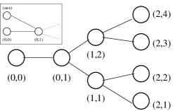
Figure 1: Spin tree of second order. The nodes are connected through edges which describe the ${XY}$ interactions defined by the Hamiltonian (1), and are identified by a double index $(a,b)$, with $(0,0)$ corresponding to the leftmost graph element. Inset: Auxiliary spin added to the BT in order to homogenise the effective couplings in the block form representation (17). The additional spin provide also a controllable trigger to start the information transfer.

In this paper we discuss the propagation of quantum information over Bifurcation Tree (BT) quantum networks. Together with the star configuration the BT configuration is arguably the most significant network topology in circuit design. The former are typically used as hubs to wire different computational devices (for an analysis of such system in the context of spin network communication see Ref. YUNG ). Star configurations have been also extensively studied for entanglement distribution HUTTON and cloning CLONE . BT networks instead are employed to route toward external memory elements (i.e. database). The information flow on unmodulated and uncontrolled BT was first discussed in Ref. FARHI while, more recently, BT quantum networks have been employed to design efficient quantum Random Access Memory elements QRAM .

The paper is organised as follows. In Sec. II we start analysing the first non trivial BT system introducing the notation and setting the problem. In Sec. III we then describe a transfer protocol that allows one to deliver a generic quantum message to any desired final edges of the second order BT network by exploiting simple end gates operations. In Sec. IV we discuss various techniques that allow us to scale up the protocol adapting it to BT of arbitrary order. The paper finally ends with the conclusions and discussion in Sec. V.

II System description

First order BT networks are just particular instances of star networks YUNG . Consequently the simplest nontrivial examples of BT networks is the second order one shown in Fig. 1. In the following we will assume the lines connecting the nodes to represent ${XY}$ (exchange) spin interactions (the results however can be generalised to include $XXZ$ or Heisenberg couplings). The resulting Hamiltonian is thus

$$H=\tfrac{J_{0}}{2}\sum_{<i,j>}(\sigma_{x}^{i}\sigma_{x}^{j}+\sigma_{y}^{i}\sigma_{y}^{j})+\sum_{j}\tfrac{\omega_{j}}{2}(\sigma_{z}^{j}+1)\;,$$ (1)

where the summation is performed over all couples $i,j$ which are connected through an edge, where $\sigma_{x,y,z}^{i}$ are the Pauli matrices associated with the $i$-th node, and where the $\omega_{i}$’s appear in consequence of the interaction with local magnetic fields (in this expression the label $i$ an $j$ stands for the joint indexes $(a,b)$ of Fig. 1). As usual BOSEREV we assume that initially the system is in the ferromagnetic “all spin down” ground state $|\O\rangle\equiv|0\cdots 0\rangle$. At time $t=0$ we then place an (unknown) qubit state $|\psi\rangle=\alpha|0\rangle+\beta|1\rangle$ on the left-most site $(0,0)$ (for instance by swapping it from an external memory). With this choice the global state of the network is now described by the vector

$$|\Psi_{\text{in}}\rangle=\alpha|\O\rangle+\beta|1_{(0,0)}\rangle\;,$$ (2)

where $|1_{(a,b)}\rangle$ represents the network state where the node $(a,b)$ is in the spin up state $|1\rangle$ while the remaining ones are in the down state $|0\rangle$, i.e.

$$|1_{(a,b)}\rangle\equiv|0\cdots 0\;1_{(a,b)}\;0\cdots 0\rangle\;.$$ (3)

Knowing that the $z$ component of the total spin is preserved by the Hamiltonian evolution of the system (i.e. $[H,S_{z}^{\textrm{tot}}]=0$) we can conclude that the dynamics is costrained in the subspace of single-flips: On this subspace $H$ acts in a very simple way that can be inferred from the graphical structure of the network, i.e.

$$H|1_{(a,b)}\rangle=\omega_{(a,b)}|1_{(a,b)}\rangle+J_{0}\sum_{(c,d)}|1_{(c,d)}\rangle\;,$$ (4)

where the sum is taken over all sites ${(c,d)}$ connected with $(a,b)$. Our goal is to find a procedure that would allow us to transfer the qubit state $|\psi\rangle$ to one the right-most sites $(2,b)$ with $b\in\{1,2,3,4\}$ of our choice, i.e.

$$|\Psi_{\text{in}}\rangle \longrightarrow |\Psi_{\text{fin}}^{(b)}\rangle\equiv\alpha|\O\rangle+\beta|1_{(2,b)}\rangle\;.$$ (5)

Following Refs. key-11 ; YUNG one could try to solve this problem by fine tuning the parameters $J_{0}$ and $\omega_{j}$ of $H$ in such a way that the free Hamiltonian evolution of the system will be able to transform $|\Psi_{\text{in}}\rangle$ into $|\Psi_{\text{fin}}^{(b)}\rangle$ after some time interval $\tau$ NOTA1 . This however is in general a quite complex calculation which entails to solve an inverse eigenvalue problem. Moreover, if any, the solutions obtained using such strategy will be arguably highly asymmetrical in the distribution of the local magnetic fields $\omega_{j}$’s. To avoid all this, here we will pursue a different approach by limiting the freedom one has in choosing the Hamiltonian parameters but, as in Refs. HASEL ; ENDG ; VGB , allowing local manipulation on the receiving node of the network (i.e. $(2,b)$). Under these conditions we can show that a simple protocol exists that realises the transformation (3) with arbitrary accuracy. It assumes an homogeneous network structure where all the ratios $\omega_{j}/J_{0}$ are chosen to be identical and equal to some fix value, and it is composed by the following three-steps:

• the system is allowed to evolve freely under the action of $H$ for some time $\tau$;

• at this point on the receiving node $(2,b)$ is performed a fast (ideally instantaneous) local transformation $\text{PS}_{(2,b)}$;

• the network is then let evolve for an extra time interval $2\tau$.

During the first step, due to the homogeneity of the Hamiltonian, the information flows along the left-right axis of the network while delocalising along the south-north axis. The value of $\tau$ is approximatively the time interval an excitation takes to travel from the leftmost node $(0,0)$ to the rightmost column formed by $(2.1)$, $(2,2)$, $(2,3)$ and $(2,4)$. The role of the local transformation $\text{PS}_{(2,b)}$ of step two is to brake the south-north symmetry of the resulting state by flipping the sign of a specific wave vector component. The system is then let evolve freely for a time interval which twice the initial one: this is approximatively the time it takes an excitation to leave the rightmost column, ”bounce back” the leftmost node, and return to the rightmost network column. Due to the symmetry brake introduced at the second step, however, the signal will now not diffuse over all the four sites $(2.1)$, $(2,2)$, $(2,3)$ and $(2,4)$, but instead it will focus on the intended receiving node $(2,b)$. A detailed description of the protocol will be presented in Sec. III.

II.1 Diagonalisation of the Hamiltonian

To solve our problem we can exploit the fact that the ground state $|\O\rangle$ of the network does not evolve to restrict ourselves to the case $\alpha=0$, i.e. $|\psi\rangle=|1\rangle$. We then simplify the structure of the Hamiltonian $(1)$ assuming all $\omega_{j}$s to be identical, i.e. $\omega_{j}\equiv\omega$. In dealing with magnetic spins this means we are applying an homogeneous magnetic field of constant strength $B\propto-\omega$ all over the system. We could set $\omega=0$, since the energy is defined up to a constant, but we let it be nonzero to guarantee that $|\O\rangle$ is the ground state of the system. We now choose the following basis for the single excitation sector, that divides the Hamiltonian in invariant blocks:

$$\text{B${}_{1}$}\left\{\begin{array}[]{l}|v_{0}\rangle\equiv|1_{(0,0)}\rangle\\ |v_{1}\rangle\equiv|1_{(0,1)}\rangle\\ |v_{2}\rangle\equiv\tfrac{1}{\sqrt{2}}(|1_{(1,1)}\rangle+|1_{(1,2)}\rangle)\\ |v_{3}\rangle\equiv\tfrac{1}{2}(|1_{(2,1)}\rangle+|1_{(2,2)}\rangle+|1_{(2,3)}\rangle+|1_{(2,4)}\rangle)\end{array}\right.$$ (10)

$$\text{B${}_{2}$}\left\{\begin{array}[]{l}|v_{4}\rangle\equiv\frac{1}{\sqrt{2}}(|1_{(1,1)}\rangle-|1_{(1,2)}\rangle)\\ |v_{5}\rangle\equiv\frac{1}{2}(|1_{(2,1)}\rangle+|1_{(2,2)}\rangle-|1_{(2,3)}\rangle-|1_{(2,4)}\rangle)\end{array}\right.$$ (13)

$$\text{B${}_{3}$}\left\{\begin{array}[]{l}|v_{6}\rangle\equiv\frac{1}{2}(|1_{(2,1)}\rangle-|1_{(2,2)}\rangle+|1_{(2,3)}\rangle-|1_{(2,4)}\rangle)\\ |v_{7}\rangle\equiv\frac{1}{2}(|1_{(2,1)}\rangle-|1_{(2,2)}\rangle-|1_{(2,3)}\rangle+|1_{(2,4)}\rangle)\;.\end{array}\right.$$ (16)

In this basis the matrix representing $H$ is given by

$$\left(\begin{array}[]{ccc}\left(\begin{array}[]{cccc}\omega&J_{0}\\ J_{0}&\omega&J\\ &J&\omega&J\\ &&J&\omega\\ \end{array}\right)\\ &\left(\begin{array}[]{cc}\omega&J\\ J&\omega\end{array}\right)\\ &&\left(\begin{array}[]{cc}\omega&0\\ 0&\omega\end{array}\right)\end{array}\right)$$ (17)

with $J\equiv\sqrt{2}J_{0}$. This shows that the evolution of the network can be effectively described as three independent linear chains, the first composed by $4$ nodes, and the other by $2$ elements each. The basic idea in deriving the above basis is that any state in the form $|1_{(a,b)}\rangle$ is decoupled from the ”singlet” superposition $\frac{1}{\sqrt{2}}(|10\rangle-|01\rangle)$ of the two nearest neighbours qubits on its right. E.g. The two states $\frac{1}{\sqrt{2}}(|1_{(2,b)}\rangle-|1_{(2,b+1)}\rangle)$ with $b=1,3$ are decoupled from the whole network and provide an alternative basis for the block $B_{3}$.
Of special interest for us is of course the block $\text{B}_{1}$ which is the only one to have an overlap with the input state (2). It is clear that the case $J_{0}=J$ would be much simpler to deal with (in this case for instance one could adapt the linear chain analysis of Refs. key-11 ; BOSE to simplify the calculation). Such option however is not possible if we assume the coupling strengths of the network to be fixed a priori. Anyway we can use a trick to obtain the same result without adjusting the coupling strength which, as discussed in the final paragraph of the present section, allows us to improve also the controllability of the setup. Suppose in fact to modify the system by adding an additional spin connected only to site $(0,1)$ with the usual ${XY}$ coupling of strength $J_{0}$, as shown in the inset of Fig. 1. With this choice the Hamiltonian (1) is replaced by

$$H_{\textrm{new}}\equiv H+\tfrac{J_{0}}{2}(\sigma_{\textrm{aux}}^{x}\sigma_{0,1}^{x}+\sigma_{\textrm{aux}}^{y}\sigma_{0,1}^{y})+\tfrac{\omega}{2}(\sigma^{z}_{\textrm{aux}}+1).$$ (18)

Now that we enlarged the Hilbert space we have to deal with the 9-dimensional space of single flips. However since the singlet state $\frac{1}{\sqrt{2}}(|1_{(0,0)}\rangle-|1_{\textrm{aux}}\rangle)$ is decoupled from the rest, if we encode the “logic” state $|1\rangle$ on the sending end of the network as $|v_{0}^{\textrm{new}}\rangle\equiv\frac{1}{\sqrt{2}}(|1_{(0,0)}\rangle+|1_{\textrm{aux}}\rangle)$ instead of using $|1_{(0,0)}\rangle$, not only we recover a dynamics costrained in an 8-dimensional space, but we obtain also an effective coupling of strength $J=\sqrt{2}J_{0}$ between $|v_{0}^{\textrm{new}}\rangle$ and $|v_{1}\rangle$ (here $|1_{\text{aux}}\rangle$ is the analogous of the states (3) with the spin up localised on the auxiliary node). The four dimensional block of our effective Hamiltonian thus becomes:

$$H_{(4)}\equiv\left(\begin{array}[]{cccc}\omega&J\\ J&\omega&J\\ &J&\omega&J\\ &&J&\omega\\ \end{array}\right)\;.$$ (19)

Following Ref. key-11 this can be easily put in diagonal form obtaining the eigenvalues

$$E_{1}\equiv\tfrac{2\omega-(\sqrt{5}+1)J}{2}\;,\qquad E_{2}\equiv\tfrac{2\omega-(\sqrt{5}-1)J}{2}\;,$$

$$E_{3}\equiv\tfrac{2\omega+(\sqrt{5}-1)J}{2}\;,\qquad E_{4}\equiv\tfrac{2\omega+(\sqrt{5}+1)J}{2}\;,$$ (20)

with the corresponding eigenstates described by the vectors

$$|e_{1}\rangle\equiv\tfrac{1}{\sqrt{5+\sqrt{5}}}\left(-1,\tfrac{1+\sqrt{5}}{2},-\tfrac{1+\sqrt{5}}{2},1\right),$$

$$|e_{2}\rangle\equiv\tfrac{1}{\sqrt{5-\sqrt{5}}}\left(1,\tfrac{1-\sqrt{5}}{2},\tfrac{1-\sqrt{5}}{2},1\right),$$

$$|e_{3}\rangle\equiv\tfrac{1}{\sqrt{5-\sqrt{5}}}\left(-1,\tfrac{1-\sqrt{5}}{2},-\tfrac{1-\sqrt{5}}{2},1\right),$$

$$|e_{4}\rangle\equiv\tfrac{1}{\sqrt{5+\sqrt{5}}}\left(1,\tfrac{1+\sqrt{5}}{2},\tfrac{1+\sqrt{5}}{2},1\right)\;,$$ (21)

(expressed in the basis $|v_{0}^{\text{new}}\rangle$, $|v_{1}\rangle$, $|v_{2}\rangle$ and $|v_{3}\rangle$).

A part from simplifying the spectral properties of the Hamiltonian, the introduction of the site aux adds also an additional feature that substantially enhances our ability of controlling the system. We have already mentioned the singlet state $\frac{1}{\sqrt{2}}(|1_{(0,0)}\rangle-|1_{\textrm{aux}}\rangle)$ is decoupled from all others vectors of the system. Therefore we can “entrap” our qubit of information at the leftmost end of the network for as much time as we like by encoding its logic $1$ component in such singlet state. When we want the transfer to start we simply apply a local Phase shift $\textrm{PS}_{\textrm{aux}}$ on the auxiliary spin that induces the mapping $|1_{\textrm{aux}}\rangle\rightarrow-|1_{\textrm{aux}}\rangle$. This will transform $\frac{1}{\sqrt{2}}(|1_{(0,0)}\rangle-|1_{\textrm{aux}}\rangle)$ into $|v_{0}^{\text{new}}\rangle$ bringing the encoded message into the four-dimensional subspace associated with the Hamiltonian (19) and allowing the first step of the above protocol to begin.

III Transfer protocol

In this section we analyse in detail the performance of the protocol defined in Sec. II. Without loss of generality we consider the case in which the receiving node is $(2,1)$, i.e. $b=1$. We recall that our aim is to obtain the transition $|v_{0}^{\text{new}}\rangle\rightarrow|1_{(2,1)}\rangle$, and we notice that

$$|1_{(2,1)}\rangle=\tfrac{1}{2}(|v_{3}\rangle+|v_{5}\rangle+|v_{6}\rangle+|v_{7}\rangle)\;.$$ (22)

The protocol: step 1.

In the first stage of the protocol the system is initialised into $|v_{0}\rangle$ and freely evolves for some time $\tau$. The goal here is to find $\omega$ and $\tau$ such that this vector is mapped into $|v_{3}\rangle$, which represents a symmetric combination in which the input excitation is spread all over the rightmost nodes of the network. As already noticed, this process is formally equivalent to the information transfer along a linear chain of $4$ spins coupled by uniform $XY$ first neighbours interactions. From Ref. key-11 we know that such transferring cannot be exact. Nevertheless the transfer fidelity can be made arbitrarily close to one. Indeed defining $U(\tau)=\exp[-iH\tau]$ and using Eq. (20) we have

$$\langle v_{3}|U(\tau)|v_{0}^{\text{new}}\rangle=\sum_{k=1}^{4}e^{-iE_{k}t}\langle v_{3}|e_{k}\rangle\langle e_{k}|v_{1}\rangle$$ (23)

$$=\tfrac{\sqrt{5}-5}{20}(e^{-iE_{1}\tau}-e^{-iE_{4}\tau})+\tfrac{\sqrt{5}+5}{20}(e^{-iE_{2}\tau}-e^{-iE_{3}\tau})\;.$$

This will be exactly one if one could find $\tau$ such that $e^{-iE_{1}\tau}=e^{-iE_{3}\tau}=-1$ and $e^{-iE_{2}\tau}=e^{-iE_{4}\tau}=1$. Even though these conditions are impossible to be satisfied exactly key-11 an approximate solution is obtained by choosing

$$\omega=\tfrac{7+\sqrt{5}}{2}\;J=\tfrac{7+\sqrt{5}}{\sqrt{2}}\;J_{0}\;,$$ (24)

and

$$\tau=\tau_{n}\equiv\frac{2n+1}{J}\pi\;,$$ (25)

with $n$ integer. Under this assumption Eq. (23) yields

$$\langle v_{3}|U(\tau_{n})|v_{0}^{\text{new}}\rangle=\tfrac{1}{2}(1+e^{-i\varphi_{n}})\;,$$ (26)

where $\varphi_{n}\equiv\sqrt{5}(2n+1)\pi$. The exponential in Eq. (26) never takes the value $1$ but, since $\sqrt{5}$ is an irrational number, approaches it indefinitely. Therefore for any $\varepsilon>0$ we can choose $n$ such that $|\langle v_{3}|U(\tau_{n})|v_{0}^{\text{new}}\rangle|\geqslant 1-\varepsilon$. As a result the state of the system, with high accuracy, is now described by the vector $|v_{3}\rangle$.

The protocol: step 2.

As a second step we act locally on the node $(2,1)$, applying the phase shift unitary transformation $\text{PS}_{21}$ which changes the sign to the state $|1_{(2,1)}\rangle$, i.e.

$$\textrm{PS}_{21}|1_{(2,1)}\rangle=-|1_{(2,1)}\rangle\;,$$ (27)

while preserving the remaining single excitation states. This can be done, for instance, by acting with an intense magnetic field which acts locally on $(2,1)$ for a time interval shorter than the characteristic times of the Hamiltonian $H$. When acting on $|v_{3}\rangle$ the unitary $\textrm{PS}_{21}$ yields the following transformation,

$$\textrm{PS}_{21}|v_{3}\rangle=\frac{1}{2}(|v_{3}\rangle-|v_{5}\rangle-|v_{6}\rangle-|v_{7}\rangle)\;.$$ (28)

This superposition contains the four states that compose the state $|1_{(2,1)}\rangle$, but the relative phases are wrong – see Eq. (22). Luckily third step fixes this issue with free evolution only.

The protocol: step 3.

Finally we just have to wait for a time $2\tau_{n}$ and the relative phases adjust themselves to give the state $|1_{(2,1)}\rangle$. In fact by explicit calculations it can be shown that

$$\begin{array}[]{l}\langle v_{3}|U(2\tau_{n})|v_{3}\rangle=\frac{1}{2}(1+e^{-i2\varphi_{n}})\simeq 1\;,\\ \\ \langle v_{k}|U(2\tau_{n})|v_{k}\rangle=-e^{-i\varphi_{n}}\simeq-1\;,\qquad\mbox{for $k=5,6,7$.}\end{array}$$ (32)

Both expressions are justified by the fact that $e^{-i\varphi_{n}}\simeq 1$, and they imply that after third step we have reached state $|1_{(2,1)}\rangle$ with as good approximation as we like.

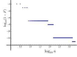
Figure 2: Minimum ”infidelity” $(1-F_{n})$ achievable according Eq. (34) for $n\in[0,N]$ as a function of $N$, i.e. $(1-F)_{\text{min}}\equiv\min_{n\leqslant N}(1-F_{n})$. Notice that already for $n=8$ we get values of $F$ greater than $1-10^{-6}$. From the plot we can infer an almost linear dependence of $(1-F)_{\text{min}}$ with respect to $N$, yielding the following (approximated) behaviour $F_{\text{min}}\sim{1-cN^{-\gamma}}$ with $\gamma\sim 1$ and $c$ being constant.

The above operations can be summarised by the application of the unitary operator

$$V_{n}\equiv U(2\tau_{n})\;\text{PS}_{(2,1)}\;U(\tau_{n})\;.$$ (33)

Therefore the resulting transfer fidelity can be expressed as

$$F_{n} \equiv |\langle 1_{(2,1)}|V_{n}|v_{0}^{\text{new}}\rangle|^{2}=\left|\tfrac{1+e^{-i\varphi_{n}}}{8}\right|^{2}$$ (34)

$$\times\left|3e^{-i\varphi_{n}}+\tfrac{1+e^{-2i\varphi_{n}}}{2}+(1+e^{-i\varphi_{n}})^{2}\right|^{2}$$

$$=\tfrac{1}{4}\cos^{2}(\varphi_{n}/2)[3-\cos^{2}(\varphi_{n}/2)]^{2}\;,$$

which approaches $1$ if $e^{-i\varphi_{n}}\simeq 1$ giving us the desired result – see Fig. 2.

IV Some ideas to scale up the system

Unfortunately our protocol doesn’t extend easily to higher-order trees (or at least we couldn’t find a simple way of doing it). The idea we pursued in trying to scale up a second order BT is to connect in some way the ends of a tree to the beginning of another. The resulting structure isn’t anymore a tree of the type described above, but it’s still a valid mean to obtain a larger number of outputs. As an example we could connect (say) two second order trees to the ends of a first order tree to obtain a $8$-outputs quantum switch, or four second order trees to the ends of a fifth second order tree to obtain a $16$-outputs quantum switch – see Fig. 3. The former setup can be solved by properly merging the protocol of Ref. YUNG with our second order BT propagation scheme: this however will require to employ non-uniform magnetic fields at least for the first spins and does not admit simple concatenation. We thus decided to focus on the second architecture which instead can be trivially concatenated to form larger setup.

Figure 3: Modified tree for the purpose of scaling up. Each rightmost qubit is accompanied now by an auxiliary, moreover all the rightmost couplings are adjusted by a factor ${1}/{\sqrt{2}}$.

We found a relatively simple way to make the required connections, but at the expenses of considering some coupling strength engineering and including antiferromagnetic interactions, which means that the “all down” configuration is no longer the ground state, although still stationary. A combination of time evolution and a phase shift will do all the work. First of all each receiving end of a tree must be accompanied by an auxiliary qubit, as done before for the sending end. In analogy to what happened introducing $(0,0)_{\textrm{aux}}$, it is easy to see that the rightmost singlets

$$|s_{2b}\rangle\equiv\frac{1}{\sqrt{2}}(|1_{(2,b)}\rangle-|1^{\textrm{aux}}_{(2,b)}\rangle)\;,$$

are isolated, while the corresponding triplets

$$|t_{2b}\rangle\equiv\frac{1}{\sqrt{2}}(|1_{(2,b)}\rangle+|1^{\textrm{aux}}_{(2,b)}\rangle)\;,$$

interact with the network and evolve, with an effective coupling strength $\sqrt{2}$ times the original one. In order for our protocol to be still valid, we need to modify the coupling strengths of the rightmost branches so that matrix (19) (now with $J_{0}=J$) remains unchanged. Moreover the local operation on the receiving end $(2,b)$ must now be performed simultaneously on $(2,b)$ and $(2,b)_{\textrm{aux}}$, i.e. we must now apply $\text{PS}_{2b}+\text{PS}_{2b}^{\textrm{aux}}$. In this way once the excitation reaches one of the end-triplets of the tree it can be trapped there with a Phase Shift on the auxiliary qubit of that site, storing information in the relative singlet. To clarify this, we outline that in this new configuration our protocol is capable of achieving the (approximate) transfer

$$\alpha|\O\rangle+\beta|1_{(0,0)}\rangle\rightarrow\alpha|\O\rangle+\beta|t_{2b}\rangle.$$ (35)

Now by applying a local phase shift $\text{PS}_{2b}^{\textrm{aux}}$ the state is transformed into

$$\alpha|\O\rangle+\beta|s_{2b}\rangle,$$ (36)

which is decoupled from the rest.
If by some means we could transfer this state to the singlet at the beginning of the next tree (denoted by primed indexes), i.e. obtain the state

$$\alpha|\O\rangle+\beta\frac{1}{\sqrt{2}}(|1_{(0^{\prime},0^{\prime})}\rangle-|1^{\textrm{aux}}_{(0^{\prime},0^{\prime})}\rangle)\equiv\alpha|\O\rangle+\beta|s_{0^{\prime}0^{\prime}}\rangle\;,$$ (37)

we could then perform the local operation $\textrm{PS}_{(0^{\prime},0^{\prime})}^{\textrm{aux}}$ to obtain the corresponding triplet state

$$\alpha|\O\rangle+\beta|t_{0^{\prime}0^{\prime}}\rangle,$$

that can be transferred along the new tree with the usual protocol.

Figure 4: The “singlet link” used to connect the outputs of the first tree to the inputs of the next column of trees (only the first one is represented here). The auxiliary qubits are not represented for simplicity.

The structure shown in Fig. 4 (that we will call “singlet link”) achieves perfect transfer between two singlets, since in the subspace $\{|s_{21}\rangle,|1_{0}\rangle,|s_{0^{\prime}0^{\prime}}\rangle\}$ it is equivalent to a chain of length 3 with constant couplings key-11 , moreover the evolution of $|t_{21}\rangle$ is decoupled from that of $|t_{0^{\prime}0^{\prime}}\rangle$ thanks to the opposite signs of the couplings along the vertical axis. The lines stand for ${XY}$ interaction of strength $J$ (ferromagnetic) and $-J$ (antiferromagnetic) respectively. As an example we have considered site $(2,1)$ of a second-order tree plus its auxiliary qubit, connected with site $(0^{\prime},0^{\prime})$ plus its auxiliary of another tree. We outline again that we are working in the subspace of single flips, as our Hamiltonian still conserves $S^{\textrm{tot}}_{z}$. In the considered example we have

$$H|s_{21}\rangle=\omega|s_{21}\rangle+\sqrt{2}J|1_{0}\rangle,$$

$$H|t_{21}\rangle=\omega|t_{21}\rangle+J|1_{(1,1)}\rangle,$$

$$H|s_{0^{\prime}0^{\prime}}\rangle=\omega|s_{0^{\prime}0^{\prime}}\rangle+\sqrt{2}J|1_{0}\rangle,$$

$$H|t_{0^{\prime}0^{\prime}}\rangle=\omega|t_{0^{\prime}0^{\prime}}\rangle+\sqrt{2}|1_{(0^{\prime},1^{\prime})}\rangle;$$

where $|t_{0^{\prime}0^{\prime}}\rangle\equiv\frac{1}{\sqrt{2}}(|1_{(0^{\prime},0^{\prime})}\rangle+|1^{\textrm{aux}}_{(0^{\prime},0^{\prime})}\rangle)$.
We can see from the above equations that once the information enters a tree through a triplet state it doesn’t come out of it until we make a Phase Shift on the desired end (and at the right time!). At this point the information goes to the singlet and propagates to the starting singlet of another tree, thanks to the singlet link, then it is transferred to the corresponding triplet with a local Phase Shift and propagation begins on the next tree. We shall repeat this procedure until information reaches the desired end on the last array of trees. Of course we must control a priori the total error due to the presence of second order trees, so to fix a “single-tree time” $\bar{\tau}$ which gives a satisfactory overall transfer fidelity.

V Conclusions

In this paper we have presented a protocol for quantum state transfer on BT spin networks of order two. As in Ref. HASEL ; VGB ; ENDG it is based on the local operations which must be performed on the receiving nodes. Differently from VGB ; ENDG however it does not involve swapping operation between the receiving nodes and external memories and arbitrarily high fidelity can be obtained in just three operational steps. Generalisation of this techniques to higher orders BT is currently under investigation: arguably this will involve more complex ends gates operations possibly on more than one of the rightmost nodes. We have however provided a simple way to scale up the problem by concatenating smaller BT network through connecting gates which can be turned on and off by simple local phase gate transformations.

We thank R. Fazio and D. Burgarth for comments and discussions. This work was in part founded by the Quantum Information program of Centro Ennio De Giorgi of the Scuola Normale Superiore.

References

- (1) G. R. Guthörlein, M. Keller, K. Hayasaka, W. Lange, and H. Walther, Nature 414, 49 (2001).
- (2) D. Leibfried, B. Demarco, V. Meyer, D. Lucas, M. Barrett, J. Britton, W. M. Itano, B. Jelenkovi, C. Langer, T. Rosenband, and D. J. Wineland, Nature 442, 412 (2003); F. Schmidt-Kaler, H. Häffner, M. Riebe , S. Gulde, T. Lancaster, C. Deuschle, C. F. Becher, B. Roos, J. Eschner, and R. Blatt , Nature 422, 408 (2003).
- (3) Yu. Makhlin, G. Schön, and A. Shnirman, Rev. Mod. Phys. 73, 357 (2001); D. V. Averin, Forthschr. Phys. 48, 1055 (2000); A. Romito, R. Fazio, and C. Bruder, Phys. Rev. B 71, 100501(R) (2005).
- (4) D. G. Angelakis, M. F. Santos, and S. Bose, Phys. Rev. A, 76, 031805(R) (2007); M. J. Hartmann, F. G. S. L. Brandão, and M. B. Plenio, Nature Physics 2, 849 (2006); A. D. Greentree, C. Tahan, J. H. Cole, and L. C. L. Hollenberg, Nature Physics 2, 856 (2006).
- (5) S. Bose, Contemporary Physics 48, 13 (2007).
- (6) S. Bose, Phys. Rev. Lett. 91, 207901 (2003).
- (7) S. Lloyd, Phys. Rev. Lett. 90, 167902 (2003).
- (8) V. Subrahmanyam, Phys. Rev. A 69, 034304 (2004).
- (9) G. M. Nikolopoulos, D. Petrosyan, and P. Lambropoulos, Europhys. Lett. 65 297 (2004).
- (10) C. Albanese, M. Christandl, N. Datta, and A. Ekert, Phys. Rev. Lett.93 230502 (2004); M. Christandl, N. Datta, A. Ekert, and A. J. Landahl, Phys. Rev. Lett. 92 187902 (2004); M. Christandl, N. Datta, T. C. Dorlas, A. Ekert, A. Kay, and A. J. Landahl, Phys. Rev. A 71, 032312 (2005).
- (11) M. -H. Yung, quant-ph/arxiv:0705.1560.
- (12) M. -H. Yung, Phys. Rev. A 74, 030303(R) (2006).
- (13) T. J. Osborne and N. Linden, Phys. Rev. A 69, 052315 (2004).
- (14) H. L. Haselgrove, Phys. Rev. A 72 062326 (2005).
- (15) D. Burgarth and S. Bose, Phys. Rev. A 71 052315 (2005); D. Burgarth, V. Giovannetti and S. Bose, J. Phys. A: Math. Gen. 38, 6793 (2005).
- (16) V. Giovannetti and D. Burgarth, Phys. Rev. Lett. 96, 010401 (2006); D. Burgarth and V. Giovannetti, Phys. Rev. Lett. 99, 100501 (2007).
- (17) D. Burgarth, V. Giovannetti and S. Bose, Phys. Rev. A 75, 062327 (2007).
- (18) A. Hutton and S. Bose, Phys. Rev. A 66, 032320 (2002); ibid. 69, 042312 (2004); arXiv: quant-ph/0408077.
- (19) G. De Chiara, R. Fazio, C. Macchiavello, S. Montangero, G. M. Palma, Phys. Rev. A 70, 062308 (2004); ibid. 72, 012328 (2005).
- (20) E. Farhi and S. Gutmann, Phys. Rev. A 58, 915 (1998).
- (21) V. Giovannetti, S. Lloyd, and L. Maccone, Phys. Rev. Lett. 100 160501 (2008); Phys. Rev. A 78, 052310 (2008).
- (22) Along this line, for instance, one could map the propagation over the network into a simpler problem by setting a subset of the s to a value much greater then the remaining constants of the systems. This will induce an effective decoupling of the selected nodes from the remaining part of the network, simplifying the underline topology.