Kinetic Equations for Transport Through Single-Molecule Transistors

Abstract

We present explicit kinetic equations for quantum transport through a general molecular quantum-dot, accounting for all contributions up to 4th order perturbation theory in the tunneling Hamiltonian and the complete molecular density matrix. Such a full treatment describes not only sequential, cotunneling and pair tunneling, but also contains terms contributing to renormalization of the molecular resonances as well as their broadening. Due to the latter all terms in the perturbation expansion are automatically well-defined for any set of system parameters, no divergences occur and no by-hand regularization is required. Additionally we show that, in contrast to 2nd order perturbation theory, in 4th order it is essential to account for quantum coherence between non-degenerate states, entering the theory through the non-diagonal elements of the density matrix. As a first application, we study a single-molecule transistor coupled to a localized vibrational mode (Anderson-Holstein model). We find that cotunneling-assisted sequential tunneling processes involving the vibration give rise to current peaks i.e. negative differential conductance in the Coulomb-blockade regime. Such peaks occur in the cross-over to strong electron-vibration coupling, where inelastic cotunneling competes with Franck-Condon suppressed sequential tunneling, and thereby indicate the strength of the electron-vibration coupling. The peaks depend sensitively on the coupling to a dissipative bath, thus providing also an experimental probe of the Q-factor of the vibrational motion.

I Introduction.

Electron transport through single-molecule transistors (SMTs) has been intensively studied theoretically in recent years (Wegewijs and Nowack, 2005; Kaat and Flensberg, 2005; Koch and von Oppen, 2005a; Donarini et al., 2006; Schultz et al., 2008; Reckermann et al., 2008, 2009; Koch and von Oppen, 2005b; Koch et al., 2006a; Cornaglia and Grempel, 2005; Koch et al., 2006b; Flensberg, 2003) driven by ongoing experimental advances (Yu et al., 2004; Natelson, 2006; Osorio et al., 2007a; Parks et al., 2007; Pasupathy et al., 2005; Park et al., 2000; Osorio et al., 2007b). One of the most distinctive features of SMTs, compared to artificially nano-structured devices such as quantum dots, is the coupling between their quantized mechanical and electronic degrees of freedom Osorio et al. (2007b). The size and shape distortions of an SMT Pasupathy et al. (2005) and its center-of-mass motion Park et al. (2000) result in sharp transport resonances whose amplitudes are governed by the quantum mechanical overlap of the corresponding mechanical wavefunctions. This Franck-Condon (FC) transport effect is of fundamental interest since it is induced by the change of molecular charge, therefore involving strong electron charging and non-equilibrium effects, in contrast to the usual FC-effect in optical spectroscopy where the charge remains unaltered. The discrete vibrational modes of a molecule are also important in assessing the atomistic details of the transport junction (Houck et al., 2005). Finally, the demonstrated control over the molecular energy levels of an SMT using a gate electrode provides interesting perspectives for realizing quantized nano-electromechanical systems (NEMS)(Sapmaz et al., 2006, 2003; Sazonova et al., 2004).

The basic FC transport picture Mitra et al. (2004) assumes single electrons to sequentially tunnel on and off the SMT. This is valid in the limit of weak tunnel coupling and for applied gate- and bias-voltages such that fluctuations of the molecular charge are not suppressed by Coulomb interaction (Coulomb blockade) or quantum confinement effects. In this limit it is sufficient to describe transport in lowest non-vanishing order perturbation theory in the tunneling and many interesting results have been reported. For instance, a well studied model in this context is the Anderson-Holstein model, consisting of a spin-degenerate level with a linear coupling (electron-vibration coupling, $\lambda$) between the charge on the level and the coordinate of a vibrational mode. When the overlap integrals between low lying vibrational states in two adjacent charge states of the SMT vanish, a suppression of single-electron tunneling (SET) occurs, called Franck-Condon blockade (Koch and von Oppen, 2005b). Here electron transport was found to take place through self-similar avalanches, leading to bunching of electrons and enhanced shot noise. Extending the basic model with a charge-dependent vibrational frequency, additional resonances occur (Koch and von Oppen, 2005a), and interference of vibrational wavefunctions was shown to lead to a suppression of the electric current at finite bias (Wegewijs and Nowack, 2005) due to a population inversion of the vibrational distribution. More complex models with (quasi-)degenerate electronic orbitals and multiple modes exhibit (pseudo-)Jahn-Teller physics. These may show rectifying behavior (Kaat and Flensberg, 2005), dynamical symmetry breaking (Donarini et al., 2006) and current suppression due to Berry phase effects (Schultz et al., 2008). Finally, distinctive transport signatures of the breakdown of the Born-Oppenheimer separation (Reckermann et al., 2008) and correlations of vibration- and spin-properties have been predicted, such as a vibration-induced spin-blockade Reckermann et al. (2009).

Since the complicated transport processes in SMTs may result in a suppression of single-electron tunneling, it becomes more urgent to understand the effect of higher order tunnel processes. Even more so since experimentally SMTs typically exhibit a significant tunnel coupling. The purpose of this paper is to set up a general method to properly describe all coherent tunnel processes in leading and next-to-leading order in the tunneling Hamiltonian. The method applies to very general molecular quantum dot models, with many quantized excitations and few relevant selection rules for transport quantities. Additionally, all molecular interactions included in the model, for instance Coulomb charging and electron-vibration, are accounted for exactly by from the outset formulating the transport equations in the basis of many-body eigenstates of the molecular Hamiltonian. The non-linear transport is obtained using the explicitly calculated non-equilibrium density matrix. A variety of next-to-leading order effects have been discussed previously. For instance, a well known signature of higher order tunneling processes is the appearance of inelastic cotunneling steps in the differential conductance, the position of which are independent of the gate voltage, which have been observed in many experiments on semi-conductor and molecular quantum-dots Yu et al. (2004); Natelson (2006); Parks et al. (2007); Osorio et al. (2007a). Additional gate-voltage dependent transport resonances have been found inside the Coulomb blockade regime (Schleser et al., 2005) and discussed theoretically (Golovach and Loss, 2004; Elste and Timm, 2007). These resonances are due to sequential tunneling events starting from states excited by inelastic cotunneling processes (“heating the molecule”), called cotunneling-assisted sequential tunneling (COSET). It was recently suggested (Lüffe et al., 2008) that these resonances can be used to experimentally estimate the decay-rate of vibrational excitations due to a coupling to a dissipative environment. Indeed, by extending the Golden-Rule approach by a next-to-leading order expansion of the T-matrix in the tunneling, it was found (Koch et al., 2006a) that the COSET features are particularly pronounced in the Anderson-Holstein model in the limit of large electron-vibration coupling. Finally, effects of electron pair-tunneling were discussed (Koch et al., 2006b) for an effective Anderson model with attractive electron-electron interaction in the Golden-Rule approach using a Schrieffer-Wolff transformation.

The method set up here captures all the aforementioned effects simultaneously. By providing a microscopic derivation we overcome some drawbacks of the methods employed in the cited works, related to accounting for broadening and renormalization of the molecular resonances, which were previously discussed in e.g. König et al. (1998); König (1999); Kubala and König (2006); Koch et al. (2006a), see also Ref. Timm (2008). The main focus of the paper is therefore on the general aspects of the transport theory. As a central result we present explicit kinetic equations from which the full molecular density matrix and transport current can be calculated. We reformulate the real-time transport theory (Schoeller and Schön, 1994; König et al., 1997) using Liouville super-operators to present a straight-forward derivation. The expressions for the transport rates are valid for a wide class of quantum-dot systems and, importantly, involve no assumptions on model-specific selection rules. We show that in such higher order calculations it is crucial to include contributions from coherent superpositions of molecular states not protected by selection rules, even when the level spacing is much larger than the tunneling broadening. The Anderson-Holstein model with a large vibrational frequency compared to the tunneling coupling, $\hbar\omega\gg\Gamma$, presents a case where this is extremely important and we demonstrate our method for this model. This is in clear contrast to lowest order perturbation theory where these so-called non-secular terms can be neglected. We are not aware of previous works pointing this out.

To maintain readability, the paper is divided into three parts: a general part II, application III and technical Appendices. In Sect. II we shortly describe the general model of a molecular quantum dot system and the basic equations of the real-time transport theory. We then discuss the central results, the explicit transport equations for the full density matrix and transport current. Detailed derivations and expressions are presented in a coherent way in the Appendices for the theoretically interested reader. In Sect. III we study in detail the specific model of a molecular transistor coupled to a localized vibrational mode, the non-equilibrium Anderson-Holstein model. We summarize and conclude in Sect. IV.

Throughout the rest of the paper we use natural units where $\hbar=k_{\text{B}}=|e|=1$ where $-|e|$ is the electron charge.

II Model and transport theory

We consider a molecule as a complex quantum dot, connected to a number of macroscopic reservoirs labeled by $r$. The electrons in the reservoirs are considered to be non-interacting, but no assumptions are made concerning the type or strength of the interactions on the molecule, as long as we can diagonalize the isolated molecular many-body Hamiltonian. The entire system is described by the Hamiltonian $H_{\text{tot}}=H+H_{\text{R}}+H_{\text{T}}$, where $H_{\text{R}}=\sum_{r}H_{r}$ and

$$H = \sum_{a}E_{a}|a\rangle\langle a|,$$ (1)

$$H_{r} = \sum_{\sigma}\int d\omega~{}\omega c_{r\sigma-\omega}c_{r\sigma+\omega},$$ (2)

$$H_{\text{T}} = \sum_{r\sigma N}\sum_{\eta=\pm 1}\sum_{a\in N}^{a^{\prime}\in({N-\eta})}\eta\int d\omega~{}T_{r\sigma\eta}^{aa^{\prime}}|a\rangle\langle a^{\prime}|c_{r\sigma\eta\omega}.$$ (3)

The Hamiltonians are written from the outset in a form which deviates from that commonly used. This allows crucial simplifications of the derivations and explicit expressions presented in the Appendices. In the molecular Hamiltonian, $H$, $|a\rangle$ denotes a general many-body eigenstate with energy $E_{a}$. We assume that we can classify these states by the number of excess electrons, $N$, on the molecule. The electron number, together with other quantum numbers depending on the model at hand (e.g. spin, magnetic and vibrational quantum numbers), are labeled by $a$. We will loosely denote by $N_{a}$ the electron number in state $a$. $H_{r}$ describes reservoir $r$ and is written in terms of continuum field operators

$$c_{r\sigma+\omega} = \sum_{k}\frac{1}{\sqrt{\rho_{r\sigma}}}\delta(\epsilon_{r\sigma k}-\omega)c_{r\sigma k},~{}~{}\eta=+,$$ (4)

$$c_{r\sigma-\omega} = \sum_{k}\frac{1}{\sqrt{\rho_{r\sigma}}}\delta(\epsilon_{r\sigma k}-\omega)c_{r\sigma k}^{\dagger},~{}~{}\eta=-,$$ (5)

where $c_{r\sigma k}^{\dagger}$ ($c_{r\sigma k}$) are the usual creation (annihilation) operators for electrons in reservoir $r$ with spin-projection $\sigma$, state-index $k$ and energy $\epsilon_{r\sigma k}$. We will refer to $\eta$ as the electron-hole (e-h) index. $\rho_{r\sigma}$ is the density of states. Inserting (4-5) into (2) one recovers the standard form of the reservoir Hamiltonian. For this one assumes that there is a unique correspondence between $k$ and $\epsilon_{r\sigma k}$. For cases where this does not hold, one labels different branches of the dispersion relation by an additional index. The tunnel Hamiltonian $H_{\text{T}}$ describes the tunneling into or out of the molecule, involving a change of the molecular state from $a^{\prime}$ to $a$. The relevant matrix elements are given by superpositions of single-particle tunneling matrix elements $t_{lr\sigma}$ and many-body amplitudes of the molecular wavefunction:

$$T_{r\sigma+}^{aa^{\prime}} = \sqrt{\rho_{r\sigma}}\sum_{l}t_{lr\sigma}\langle a|d_{l\sigma}^{\dagger}|a^{\prime}\rangle,$$ (6)

$$T_{r\sigma-}^{aa^{\prime}} = \sqrt{\rho_{r\sigma}}\sum_{l}t^{*}_{lr\sigma}\langle a|d_{l\sigma}|a^{\prime}\rangle=\left(T_{r\sigma+}^{a^{\prime}a}\right)^{*}.$$ (7)

Here $l$ labels a single particle basis for the molecule with corresponding creation / annihilation operator $d_{l\sigma}^{\dagger},d_{l\sigma}$. Note that the density of states is incorporated in $T_{r\sigma\eta}^{aa^{\prime}}$, simplifying many expressions. The spectral densities $\Gamma^{ab,a^{\prime}b^{\prime}}_{r\sigma}=2\pi T_{r\sigma+}^{aa^{\prime}}T_{r\sigma-}^{b^{\prime}b}$, thus represent the set of relevant energy scales for the tunneling. Both $\rho_{r\sigma}$ and $t_{lr\sigma}$ are assumed to be energy independent. This is the most relevant physical limit and presents no principle limitation of the presented method (only numerical). Charge conservation implies the selection rule, $N_{a}-N_{a^{\prime}}=1$, which is contained in $\langle a|d_{l\sigma}^{\dagger}|a^{\prime}\rangle\propto\delta_{N_{a},N_{a^{\prime}}+1}$. This is the only selection rule assumed. A Fermion sign, $\eta$, appears in Eq. (3) since we always write the reservoir operator to the right of the projector. However, one can show that this exactly cancels in all expressions involving an average over the reservoir degrees of freedom. It cancels with an extra Fermion sign appearing when disentangling the dot and reservoir operators, using that an equal number of creation and annihilation operators must occur to give a non-zero average, see Ref. Schoeller (2009) for a proof. We can therefore discard the sign $\eta$ from the outset, and everywhere treat dot and lead operators as commuting, greatly simplifying the calculation of signs.

II.1 Kinetic Equation

A microscopic molecular system coupled to macroscopic reservoirs is completely described by its reduced density operator $P(t)$, obtained by averaging the total density operator over the reservoir degrees of freedom, $P(t)=\text{Tr}_{\text{R}}\rho(t)$. The reduced density operator evolves in time according to a quantum kinetic equation. The presence of strong non-equilibrium effects (non-linear transport) and strong local interactions (Coulomb, electron-vibration, etc.) makes the calculation of the transport rates occurring in this equation a cumbersome task. Here our goal is to derive explicit expressions for the next-to-leading order transport rates in terms of the parameters $E_{a},T^{aa^{\prime}}_{r\sigma\eta}$ of the Hamiltonians (1–3) and the statistical properties of the electrodes $T$ (temperature) and $\mu_{r}$ (chemical potential). The real-time transport theory, developed in (Schoeller and Schön, 1994; König et al., 1997) and extended by several groups (Thielmann et al., 2005; Weymann et al., 2005; Kubala and König, 2006), provides straightforward rules for the calculation of the transport rates using a diagrammatic representation on the Keldysh contour, avoiding any spurious regularization problems. This technique has been simplified further by using special Liouville super-operators and corresponding diagrams in the context of a non-equilibrium renormalization group approach Schoeller (2009); Korb et al. (2007). For clarity we discuss the general aspects here, whereas the important but cumbersome expressions are coherently derived and presented in the Appendices. The starting point is the time evolution of the density operator of the total system, molecule + reservoirs:

$$\rho(t)=e^{-iL_{\text{tot}}t}\rho(0).$$ (8)

Here the Liouvillian super-operators in $L_{\text{tot}}=L+L_{\text{R}}+L_{\text{T}}$, act on an arbitrary operator $A$ by forming a commutator with the Hamiltonian, e.g. $LA=[H,A]$. We assume the system to be decoupled at the initial time $t=0$, such that the density operator factorizes, $\rho(0)=P(0)\rho_{\text{R}}$ where $\rho_{\text{R}}=\prod_{r}\rho_{r}$ and $\rho_{r}$ describes reservoir $r$. Each reservoir is assumed to remain in internal equilibrium independently and is described by a grand-canonical ensemble at all times. When a bias voltage is applied to the system, causing the chemical potentials of different leads to differ, this puts an inhomogeneous “boundary condition” on the molecular density operator and drives it out of equilibrium. We now take the Laplace transform of Eq. (8) and trace out the reservoirs

$$P(z) = \underset{\text{R}}{\text{Tr}}\int_{0}^{\infty}dte^{izt}e^{-iL_{\text{tot}}t}P(0)\rho_{\text{R}}$$ (9)

$$= i\underset{\text{R}}{\text{Tr}}\frac{1}{z-L_{\text{R}}-L-L_{\text{T}}}P(0)\rho_{\text{R}}$$ (10)

$$= \frac{i}{z-L-iW(z)}P(0),$$ (11)

where the last expression is obtained by expanding the denominator in (10) in powers of the tunneling Liouvillian, $L_{\text{T}}$, carrying out the trace over the reservoirs and re-summing the series, see Appendix A for details. Here $iW(z)$ is a (super-operator) self-energy and $L+iW(z)$ describes the molecular density operator in the presence of the reservoirs. If Eq. (11) is transformed back to the time-domain, $W(t-t^{\prime})$ appears as a kernel in the integro-differential equation for $P(t)$

$$\dot{P}(t)=-iLP(t)+\int_{0}^{t}dt^{\prime}W(t-t^{\prime})P(t^{\prime}),$$ (12)

assuming that the Laplace transform of $W(t-t^{\prime})$ exists. We are exclusively interested in the stationary state at $t\rightarrow\infty$ (asymptotic solution) of the molecular density operator, i.e. the zero frequency limit $z\rightarrow i0$ where the imaginary infinitesimal physically originates from the adiabatic switching on of the tunneling. Assuming that a unique stationary state exists and using $\text{lim}_{t\rightarrow\infty}P(t)=-i\text{lim}_{z\rightarrow i0}zP(z)$, Eq. (11) gives the standard form Schoeller and Schön (1994); König (1999); Schoeller (2009) of the stationary state equation:

$$0=\left(-iL+W\right)P.$$ (13)

Here, and in the rest of the paper, we use the notation $W=\text{lim}_{z\rightarrow i0}W(z)$ and $P=\text{lim}_{t\rightarrow\infty}P(t)$. Supplemented with the probability normalization condition $\text{Tr}_{\text{M}}P=1$, where $\text{Tr}_{\text{M}}$ is the trace over the molecular degrees of freedom, this uniquely determines the stationary state. The normalizability derives from the general property of the kernel $\text{Tr}_{\text{M}}WA=0$ for any operator $A$. Matrix elements of a super-operator, $S$, are defined according to

$$S^{a^{\prime}b^{\prime}}_{ab}\equiv\langle a|\left(S|a^{\prime}\rangle\langle b^{\prime}|\right)|b\rangle,$$ (14)

meaning that we first act with $S$ on a projector $|a^{\prime}\rangle\langle b^{\prime}|$, generating a new operator, and subsequently take matrix elements of this. In the basis of the many-body eigenstates of the isolated molecule the molecular Liouvillian is

$$L_{ab}^{a^{\prime}b^{\prime}}=(E_{a}-E_{b})\delta_{aa^{\prime}}\delta_{bb^{\prime}}.$$ (15)

Our main objective is to calculate the expectation value of the electron current flowing out of reservoir $r$ into the molecule, $I_{r}(t)=\text{Tr}\hat{I}_{r}\rho(t)$ where Tr is the trace over the full system and $\hat{I}_{r}=-\frac{d}{dt}N_{r}=-i[H_{\text{T}},N_{r}]$, with $N_{r}$ being the number operator for electrons in reservoir $r$. As is shown in Appendix A, this expectation value can be obtained from a kernel similar to $W$ and the density operator. In the stationary state: $I_{r}=\text{Tr}_{\text{M}}\{W_{I_{r}}P\}$, where the current kernel, $W_{I_{r}}$, contains the subset of tunneling processes described by $W$ which contribute to the current through reservoir $r$. We can now write down the generalized, formally exact, master equations

$$0 = \sum_{a^{\prime}b^{\prime}}\left[-iL_{ab}^{a^{\prime}b^{\prime}}+\sum_{k=1}^{\infty}\left(W^{(2k)}\right)_{ab}^{a^{\prime}b^{\prime}}\right]P_{a^{\prime}b^{\prime}},$$ (16)

$$1 = \sum_{a}P_{aa},$$ (17)

$$I_{r} = \sum_{a}\sum_{a^{\prime}b^{\prime}}\sum_{k}\left(W_{I_{r}}^{(2k)}\right)^{a^{\prime}b^{\prime}}_{aa}P_{a^{\prime}b^{\prime}}.$$ (18)

Here we have expanded the kernels in even order terms $2k$ in the tunneling Liouvillian accounting for coherent $k$-electron tunnel processes (odd orders vanish when tracing over the reservoirs since the tunneling Hamiltonian is linear in reservoir field operators). Eq. (16–18) compactly formulate the transport problem. The first central result of this paper is the explicit evaluation of the kernels $W^{(2)}$ and $W^{(4)}$ as given in Appendix C (Eq. (58)) and D (Eq. (D)), accounting for coherent single- and two-electron tunneling processes. Their detailed form is not needed here, but an important property of these expressions is that they are finite by construction for any system parameters and applied voltages at non-zero temperature: no divergences occur and no by-hand regularization is required at any stage of the calculation as is the case in the Golden-Rule T-matrix approach Koch et al. (2006a). Of course, the finite temperature must be chosen sufficiently large compared to the tunneling couplings ($\Gamma\ll T$) to avoid the breakdown of perturbation theory.

For the solution of the kinetic equation it is important to know whether the molecular density matrix is diagonal in certain quantum numbers due to a conservation law. The only such law explicitly enforced here concerns the total charge in reservoirs + molecule: $[H_{\text{tot}},N_{\text{tot}}]=0$. As is shown in Appendix B, the matrix elements of $W^{a^{\prime}b^{\prime}}_{ab}$ vanish unless the charge differences are equal: $N_{a^{\prime}}-N_{b^{\prime}}=N_{a}-N_{b}$. With the assumption that the density matrix is diagonal with respect to charge at $t=0$, before the coupling to the reservoirs is switched on, it is guaranteed to remain so at all times. In a similar way any conserved quantity of the total system encodes selection rules in the tunneling matrix elements ensuring that the density matrix remains diagonal in the corresponding molecular quantum number. For example, for the Anderson-Holstein model studied in Sect. III the conservation of total spin-projection, $S_{z}$, leads to a density matrix which is diagonal in the spin-projection of the molecule, $s_{z}$.

II.2 Solution of the Kinetic Equation

The solution of equations (16-18) with perturbatively calculated kernels (up to a finite order) for the full molecular density matrix requires some care for models with excited states and tunnel matrix elements without strict selection rules. The present section is therefore devoted to deriving the correct and well-behaved master equations in next-to-leading order perturbation theory. First we rewrite the equations by collecting the elements of the density operator into a vector, $\mathbf{P}$, and the elements of the rate super-operators into matrices $\mathbf{W},\mathbf{W}_{I_{r}},\mathbf{L}$ acting on this vector. Up to 4th order in the perturbation expansion the equations can now be written as

$$\mathbf{0} = \left(-i\mathbf{L}+\mathbf{W}^{(2)}+\mathbf{W}^{(4)}\right)\mathbf{P},$$ (19)

$$1 = \mathbf{e}^{T}\mathbf{P},$$ (20)

$$I_{r} = \mathbf{e}^{T}\left(\mathbf{W}_{I_{r}}^{(2)}+\mathbf{W}_{I_{r}}^{(4)}\right)\mathbf{P}.$$ (21)

The trace in Eq. (17), (18) is effected by the multiplication with the auxiliary vector $\mathbf{e}^{T}=(1,\ldots,1,0,\ldots,0)$ to sum up all vector elements corresponding to diagonal density-matrix elements. The sum-rule on the kernel reads $\mathbf{e}^{T}\mathbf{W}=\mathbf{0}^{T}$.

II.2.1 Elimination of Non-Diagonal Elements

The crucial assumption for the following discussion is that the spectrum is free from accidental degeneracies in the following sense: all pairs of states $a\neq b$ which have non-zero non-diagonal density matrix elements $P_{ab}$ are well separated in energy on the scale set by the tunneling rates. Models for molecular transistors with discrete vibrational modes, such as the Anderson-Holstein model, satisfy this condition, provided that the vibrational level-spacing is larger than the tunneling coupling, since spin-selection rules generally prohibit coherence between the degenerate spin-states, unless broken by e.g. magnetic anisotropy or spin-polarization of the electrodes. One can always eliminate the non-diagonal elements and incorporate their effect in a correction to the rates coupling diagonal elements. To this end we collect diagonal ($d$) and non-diagonal ($n$) density matrix elements into separate vectors $\mathbf{P}_{d}$ and $\mathbf{P}_{n}$, separate (19) into blocks and denote $\mathbf{W}=\mathbf{W}^{(2)}+\mathbf{W}^{(4)}$:

$$\left[\begin{array}[]{c}\mathbf{0}_{d}\\ \mathbf{0}_{n}\end{array}\right]=\left[\begin{array}[]{cc}\mathbf{W}_{dd}&\mathbf{W}_{dn}\\ \mathbf{W}_{nd}&\mathbf{W}_{nn}-i\mathbf{L}_{nn}\end{array}\right]\left[\begin{array}[]{c}\mathbf{P}_{d}\\ \mathbf{P}_{n}\end{array}\right].$$ (28)

It is clear from (15) that $\mathbf{L}$ is only non-zero in the $nn$ block. The sum-rule implies

$$\mathbf{e}_{d}^{T}\mathbf{W}_{dd} = \mathbf{0}_{d}^{T},$$ (29)

$$\mathbf{e}_{d}^{T}\mathbf{W}_{dn} = \mathbf{0}_{n}^{T},$$ (30)

where the multiplication with the vector $\mathbf{e}^{T}_{d}=(1,\ldots,1)$ sums up all $d$-vector elements. We can now eliminate processes into the non-diagonal sector of the density-matrix by solving the equation from the lower block for the non-diagonal part of the density matrix, $\mathbf{P}_{n}$, and inserting this back into the equation in the upper block for the diagonal part. Due to the clear separation of energy scales (non-degenerate spectrum) we can expand in the small quantity $\mathbf{W}_{nn}\mathbf{L}_{nn}^{-1}$. Consistently neglecting terms of order $>H_{\text{T}}^{4}$ we then obtain an effective equation for $\mathbf{P}_{d}$:

$$\mathbf{W}_{d}\mathbf{P}_{d} = 0,$$ (31)

$$\mathbf{e}_{d}^{T}\mathbf{P}_{d} = 1,$$ (32)

$$\mathbf{W}_{d} = \mathbf{W}_{dd}^{(2)}+\mathbf{W}_{dd}^{(4)}-i\mathbf{W}_{dn}^{(2)}\mathbf{L}_{nn}^{-1}\mathbf{W}_{nd}^{(2)}.$$ (33)

The diagonal elements of the density matrix (vector of probabilities) thus satisfy what looks like a classical rate-equation, but with the effective rates (33). A completely analogous calculation for the correction to the current from non-diagonal elements gives

$$I_{r} = \mathbf{e}^{T}_{d}\left(\mathbf{W}_{I_{r}}\right)_{d}\mathbf{P}_{d},$$ (34)

$$\left(\mathbf{W}_{I_{r}}\right)_{d}=$$

$$\left(\mathbf{W}_{I_{r}}^{(2)}\right)_{dd}+\left(\mathbf{W}_{I_{r}}^{(4)}\right)_{dd}-i\left(\mathbf{W}_{I_{r}}^{(2)}\right)_{dn}\mathbf{L}_{nn}^{-1}\mathbf{W}_{nd}^{(2)}.$$ (35)

It can easily be shown that (33) and (II.2.1) are real, ensuring that the diagonal elements of the density matrix as well as the current are real. Due to Eq. (29–30) the effective rate matrix satisfies the sumrule $\mathbf{e}_{d}^{T}\mathbf{W}_{d}=\mathbf{0}^{T}$, so that Eq. (31) with Eq. (32) determine the unique stationary solution for the vector of diagonal density matrix elements (probabilities). Eq. (31-II.2.1) form another central result of this work and we comment on their significance and importance. The advantage of the formulation in terms of effective rates, compared to solving Eq. (19–21) directly, is threefold: (i) the effective rate matrices include the effects of coherences only up to order $H_{\text{T}}^{4}$, just as the other effects of tunneling; (ii) it makes it explicit that the 2nd order coherences effectively give 4th order effects in the rates for the occupations, something which is hidden in Eq. (19); (iii) it shows that the large matrix $\mathbf{W}_{nn}$, as well as all 4th order matrices which are not diagonal in initial and final state indices, need not be evaluated, significantly simplifying the calculation. The appearance of the correction in the effective rate has an intuitive physical meaning in the time-domain: it corresponds to a process starting ($\mathbf{W}_{nd}$) and ending ($\mathbf{W}_{dn}$) in a diagonal state, through two tunnel processes. In the intermediate non-diagonal state the free evolution involves rapid coherent oscillations at the Bohr-frequencies contained in $\mathbf{L}_{nn}$ (see (15)). Due to the latter, these so-called non-secular terms Blum (1996) should be neglected in a lowest order approximation. However, these correction terms from coherences between non-degenerate states, although formally containing only 2nd order rates, contribute in 4th order to the occupancies, where they are crucial unless special model properties (conservation laws) make the matrix $\mathbf{W}_{dn}$ vanish exactly. They scale in the same way as processes described by $\mathbf{W}_{dd}^{(4)}$ when one uniformly reduces the tunneling matrix elements. Finally, we have found by numerical calculations for several model systems that partial cancellations between the non-diagonal correction terms and diagonal 4th order terms are crucial for obtaining a physical result: if these corrections are excluded one obtains SET-like resonances in the Coulomb-blockade regime below the inelastic cotunneling threshold. These are artifacts due to incorrect, large occupations of the excited states, even at zero bias voltage. Depending on the parameters of the model, negative occupation probabilities may even result, particularly when the tunneling amplitudes (6-7) vary strongly from state to state. Accounting for the non-diagonal correction terms no such artifacts occur. Models for SMTs are typical systems where the neglect of these non-diagonal corrections results in dramatic, spurious effects in the occupations and current.

Summarizing: in the limit of large level-spacing, Eq. (31–II.2.1) are the correct expressions for the occupation probabilities and current. The corrections from 2nd order non-diagonal terms contribute only in 4th order in $H_{T}$: in a consistent 2nd order calculation they must be omitted whereas in a 4th order calculation they must be kept unless all non-diagonal elements vanish due to selection rules.

II.2.2 Calculation of Diagonal Elements

Having eliminated the non-diagonal elements, the remaining problem is the solution of the kinetic equation for the diagonal elements (31–32) only. This requires some care since the effective rates (33) contain both 2nd and 4th order terms, as was discussed in previous works (Weymann et al., 2005; Becker and Pfannkuche, 2008) (where corrections from non-diagonal elements were exactly zero due to selection rules). The problem is most easily understood from a simple example. Fig. 1(a) shows the result of 4th order perturbation theory for the single-level Anderson model in a magnetic field by solving Eq. (31–II.2.1) (due to spin-conservation $\mathbf{W}_{dn}^{(2)}=\mathbf{0}$ and non-diagonal elements play no role) and Fig. 1(b) indicates relevant tunneling processes in regions (1), (2) and (3) in (a).

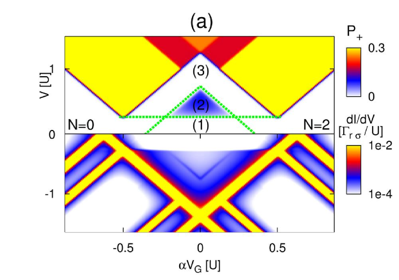
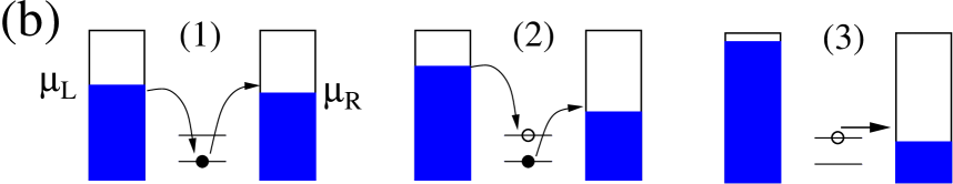
Figure 1: (Color online). (a): Occupation of excited spin-state, $P_{+}$ (top, positive bias) and differential conductance (bottom, negative bias) for the single-level Anderson model where the spin degeneracy is lifted by an applied magnetic field. Here $\Gamma_{\text{L}\sigma}=\Gamma_{\text{R}\sigma}=10^{-2}T=5\times 10^{-5}U$, where $U$ is the charging energy, and $\epsilon_{\uparrow}-\epsilon_{\downarrow}=50T$. (b): Energy diagrams in the regions (1), (2) and (3), separated by green dashed lines in (a). In (1) only elastic cotunneling is energetically possible. In (2) also inelastic cotunneling can take place, but the only way for the excited system to return to the ground state is by another inelastic cotunneling process. In (3) the excited state can be emptied also by sequential tunneling processes (COSET).

In region (2) the excited spin-state can be populated by 4th order processes (inelastic cotunneling). Since sequential tunneling out of this state is only possible at larger bias (region (3)), it can only relax by another inelastic cotunneling process back into the ground state. This latter process would not be included if one insists on an order-by-order solution, i.e. expand also the occupation vector in powers of $H_{\text{T}}$: $\mathbf{P}=\delta\mathbf{P}^{(0)}+\delta\mathbf{P}^{(2)}$, solve for $\delta\mathbf{P}^{(0)}$ and $\delta\mathbf{P}^{(2)}$ separately and discard the term $\mathbf{W}^{(4)}_{dd}\delta\mathbf{P}^{(2)}$ in (31), which is formally of order 6. Such an approach thus breaks down since the excited state is “pumped” up by inelastic tunneling, but not allowed to relax by 4th order processes, yielding an unphysical solution: $\mathbf{W}^{(4)}_{dd}\delta\mathbf{P}^{(0)}$ provides an inflow into the excited spin-state, but no outflow since $\delta\mathbf{P}^{(0)}$ is only finite for the ground state, resulting in an artificially large correction $\delta\mathbf{P}^{(2)}$. Eq. (31) on the other hand has well behaved solutions, in which the occupancy of the excited spin-state is determined by the competition of in- and out-going 4th order rates. We emphasize that the problem with the order-by-order solution is not of a numerical nature and occurs even if the equations are solved analytically. It is of a general nature and occurs whenever all lowest order rates connected to some state are suppressed. Ref. (Weymann et al., 2005) suggests dividing the Coulomb diamond into different regions, adapting the solution of the master equations thereafter, e.g. using the order-by-order solution in the SET regime only. However, for a general SMT model such a division is not possible since even in the SET regime some rates may be suppressed by e.g. Franck-Condon or magnetic blockade effects. Always solving Eq. (31) guarantees a physical solution in the sense that in- and out-going rates of all states are treated on an equal footing and the accuracy of the method is only limited by the order of the perturbation expansion of the kernel $W$.

III Non-equilibrium Anderson-Holstein model

We now turn our focus to the Anderson-Holstein model, choosing the specific form of the molecular Hamiltonian (1)

$$H=\epsilon\sum_{\sigma}d^{\dagger}_{\sigma}d_{\sigma}+\frac{U}{2}\hat{n}(\hat{n}-1)+\omega(b^{\dagger}b+\frac{1}{2}).$$ (36)

The first two terms describe an electron in a single molecular orbital with electron operators $d^{\dagger}_{\sigma},d_{\sigma}$ for spin $\sigma$ and $\hat{n}=\sum_{\sigma}d^{\dagger}_{\sigma}d_{\sigma}$ denotes the number of excess electrons on the SMT. The last term describes the quantized vibration of the SMT through the operators $b^{\dagger},b$. The eigenstates $|a\rangle$ in Eq. (1) thus have an electronic and a vibrational part, $|a\rangle=|e\rangle|m_{e}\rangle$, where $|e\rangle=|0\rangle$, $|\uparrow\rangle$, $|\downarrow\rangle$, $|\uparrow\downarrow\rangle$ denotes the electronic state with $N=0,1,2$ excess electrons on the molecule, and $|m_{e}\rangle$ labels the state of the oscillator.

We have written Eq. (36) in the standard polaron-basis where $\epsilon$ denotes the experimentally controllable effective energy level and $U$ denotes the effective charging energy, both containing polaron-shift corrections Cornaglia and Grempel (2005). The dimensionless electron-vibration coupling, denoted by $\lambda$, appears in an operator which displaces the vibrational states by $\sqrt{2}\lambda$ along the vibrational coordinate (normalized to the zero-point amplitude), whenever an electron tunnels from the electrodes onto the molecule, see Fig. 2. Thus the addition of an electron to the SMT induces a transition $N\rightarrow N+1$, accompanied by a change of its vibrational state $m^{\prime}\rightarrow m$. The matrix element for this process is reduced relative to the pure electronic tunneling amplitude by the Franck-Condon overlap of vibrational wavefunctions in two different charge states of the SMT:

$$f_{mm^{\prime}} = \langle m|e^{-\lambda(b^{\dagger}-b)}|m^{\prime}\rangle$$

$$= \left(-\lambda\right)^{m-m^{\prime}}e^{-\frac{\lambda^{2}}{2}}\sqrt{\frac{m^{\prime}!}{m!}}L_{m^{\prime}}^{m-m^{\prime}}(\lambda^{2}),$$

for $m\geq m^{\prime}$ (replace $m\leftrightarrow m^{\prime}$ for $m<m^{\prime}$) where $L_{j}^{i}(x)$ is the generalized Laguerre polynomial.

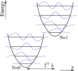
Figure 2: (Color online). Vibrational potentials in charge state $N=0$ and $N=1$ and lowest corresponding vibrational wavefunctions. The minimum of the potentials are shifted along the vibrational coordinate $x$ by $\sqrt{2}\lambda$ (in units of the zero-point amplitude of the oscillator).

The dependence of the Franck-Condon factors on $m$ and $m^{\prime}$ was discussed in detail in (Wegewijs and Nowack, 2005). For a tunneling event starting from the vibrational ground state, $m^{\prime}=0$, the Franck-Condon factors have a significant amplitude for $\lambda^{2}-\lambda\lesssim m\lesssim\lambda^{2}+\lambda$, corresponding to classically allowed transitions. More generally, for moderate to strong coupling there are broad regions in the $m,m^{\prime}$ plane, bounded by the so-called Franck-Condon parabola, where vibration assisted transitions have significant amplitude. These finite amplitudes for transitions to a range of vibrational states make the coherence between all pairs of these states important for the 4th order calculation, even though they are non-degenerate (on the scale of the tunneling broadening), i.e. there are many non-zero elements of $\mathbf{W}_{dn}$ and $\mathbf{W}_{nd}$ in (33).

Here we are interested in transport close to a charge degeneracy point, accounting for the fact that the charging energy together with the confinement-induced level-spacing typically constitute the largest energy scales in SMTs. We therefore restrict the model to electronic states with charge $N=0,1$, equivalent to taking $U\rightarrow\infty$ in Eq. (36). Without loss of generality we take $\epsilon=-\alpha V_{\text{G}}$, where $\alpha$ is the gate-coupling factor, i.e. we associate $\epsilon=0$ with zero gate voltage. The tunneling matrix elements for an electron tunneling onto the molecule are given by $T_{r\sigma+}^{aa^{\prime}}=\delta_{s_{z}\sigma}\sqrt{\rho}t_{r}f_{mm^{\prime}}$, where the eigenstates are labeled by the quantum numbers $a=(s_{z},m)$ in the $N=1$ charge state and $a^{\prime}=(0,m^{\prime})$ in the $N=0$ charge state, with $s_{z}$ denoting the spin-projection of the molecule. We have everywhere used $\omega=40T=10^{4}\Gamma_{\text{M}}$, where $\Gamma_{\text{M}}$ is the maximum sequential tunneling rate, i.e. $\Gamma_{\text{M}}=\Gamma\times\text{max}(|f_{mm^{\prime}}|^{2})$ and $\Gamma=|2\pi\sqrt{\rho}t_{L}|^{2}=|2\pi\sqrt{\rho}t_{R}|^{2}$ is the pure electronic tunneling rate for symmetric coupling to the left and right electrodes. We set the width of the conduction band to $D=250\omega$.

III.1 Intermediate Coupling

The differential conductance as a function of gate and bias voltage is shown in Fig. 3 in the case of intermediate electron-vibration coupling, $\lambda=1$ in (a) and $\lambda=2$ in (b).

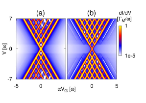
Figure 3: (Color online). Differential conductance as a function of gate and bias voltage close to the $N=0\leftrightarrow N=1$ degeneracy point, for $\lambda=1$ (a) and $\lambda=2$ (b). In the logarithmic scale the lower end has to be chosen positive, preventing negative values from being correctly displayed, see e.g. white areas inside the sequential tunneling region in (a) which actually correspond to very weak negative differential conductance (NDC).

The regimes where SET processes give the main contribution to the current are triangle-shaped regions emanating from the point $V_{\text{G}}=0$, where the energy for electron addition without changing the vibrational quantum number lies between the electro-chemical potentials. Due to the quantized nature of the vibration of the SMT, additional sharp peaks appear in the differential conductance, associated with a change of the vibrational quantum number. Since in the SET-regime this is accompanied by a change in the charge, the positions of these peaks depend linearly on the applied gate voltage. At the $k$-th resonance line (counting from $V=0$) a new set of transitions becomes energetically allowed, where the vibrational quantum number changes by $k$ upon (dis)charging.

Outside these two regimes, SET processes are suppressed by Coulomb blockade and one charge state is stable. Here no features are seen in a plot corresponding to Fig. 3 calculated to lowest non-vanishing order (not shown, see e.g. Nowack and Wegewijs ; Koch and von Oppen (2005b)). However, since we include all next-to-leading order processes, distinct features appear in this region, which we now discuss. When the bias voltage reaches the vibrational level spacing, inelastic cotunneling processes exciting one vibrational quantum become energetically allowed. Due to the harmonic spectrum, this makes every excited vibrational state for fixed $N$ accessible through a sequence of such tunneling processes: the molecular vibration is driven out of equilibrium. Each inelastic process involves the virtual occupation of an adjacent charge state with an arbitrary vibrational excitation number. The onset of inelastic cotunneling is seen as steps in the differential conductance, whose positions are independent of the gate voltage since the process does not change the charge state of the SMT. The magnitude of the steps however depend on the gate voltage since the occupation of the virtual intermediate state is algebraically suppressed with the energy of this state. Similarly, at $V=k\omega$ inelastic cotunneling processes exciting $k$ vibrational quanta become possible. The corresponding 2nd and 3rd inelastic cotunneling steps are weakly seen for $\lambda=2$, while, for the tunneling coupling considered here, the suppression of the corresponding Franck-Condon factors renders them invisible for $\lambda=1$.

A striking difference between Fig. 3(a) and (b) is the appearance of gate-dependent lines inside the Coulomb blockade region in (b). The gate-dependence indicates that these lines are due to processes changing the charge state of the SMT, but they cannot be due to SET processes starting out from the vibrational ground state, since these are exponentially suppressed by Boltzmann factors (energy conservation). They originate instead from SET processes starting out from an excited vibrational state, which has previously been occupied by inelastic cotunneling processes. This sequence of leading and next-to-leading order tunneling processes is called cotunneling-assisted sequential tunneling (COSET)  (Golovach and Loss, 2004; Schleser et al., 2005; Koch et al., 2006a; Lüffe et al., 2008; Aghassi et al., 2008), in the context of inelastic electron tunneling spectroscopy (IETS) often referred to as phonon absorption peaks, see Ref. (Galperin et al., 2007) and references therein. For even larger electron-vibration coupling these features become more pronounced as discussed in the next section.

III.2 Cross-over to Strong Coupling

The results of the calculations for larger electron-vibration coupling are shown in Fig. 4, where $\lambda=3$ in (a) and $\lambda=4$ in (b).

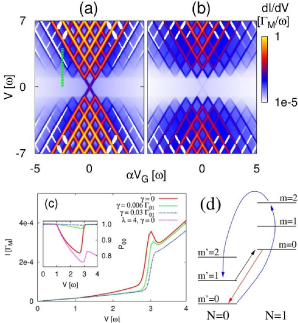
Figure 4: (Color online). (a) and (b): Differential conductance as a function of gate and bias voltage for strong electron-vibration coupling, $\lambda=3$ in (a) and $\lambda=4$ in (b). For some values of the applied voltages the COSET processes result in closely spaced positive and negative differential conductance peaks, corresponding to peaks in the current. (c): Current as a function of bias voltage for $\lambda=3$ along the dashed green line in (a), where the COSET processes give rise to a step + peak feature. As the vibrational relaxation rate, $\gamma$, is increased relative to $\Gamma_{01}=\Gamma|f_{01}|^{2}$ the peak vanishes, while the step remains. Inset: occupation of the vibrational ground state of the $N=0$ charge state, including also the result for $\lambda=4$ without relaxation. (d): Sketch of lowest vibrational states in the $N=0,1$ charge states. An example of a COSET process contributing to the step + peak in (c) consists of an inelastic cotunneling process (blue arrows), followed by a sequential tunneling process (black arrow) into the vibrational ground state of the unstable charge state ($N=1$). This may in turn sequentially relax (red arrow) to the vibrational ground state of the stable charge state ($N=0$).

The most obvious consequence of a large electron-vibration coupling is the suppression of the low bias conductance. This Franck-Condon blockade stems from exponentially vanishing overlap integrals (Franck-Condon factors) between low-lying vibrational states (Braig and Flensberg, 2003; Koch and von Oppen, 2005b; Pistolesi and Labarthe, 2007) which is seen in Fig. 4 as a suppression of the degeneracy point peak (the differential conductance peak at $V=V_{\text{G}}=0$). In the case of an equilibrium vibrational distribution and lowest order transport calculation, the current would increase exponentially with increasing bias voltage, until the blockade is lifted at around $V/2=(\lambda^{2}-\lambda)\omega=m$ corresponding to the first large Franck-Condon factor $f_{m0}$. However, when the vibrational distribution is pushed out of equilibrium by sequential tunneling processes, this significantly enhances the current compared to the case of equilibrium vibrations. Additionally, when next-to-leading order transport processes are taken into account, which was done using the Golden-Rule T-matrix approach in Ref. (Koch et al., 2006a) to study the strong coupling regime ($\lambda=4$ and $\lambda=5$), elastic and inelastic cotunneling processes change the exponential suppression into an algebraic one. Cotunneling processes take place through high lying virtual intermediate vibrational states ($m\sim\lambda^{2}$) which have a large overlap with the vibrational ground state, and the suppression of these processes is only algebraic with respect to the energy of the virtual state, and therefore with respect to $\lambda$.

The lowest inelastic cotunneling step is clearly seen for both $\lambda=3$ and $\lambda=4$. Additionally we find an anomalous signature of COSET processes. For low bias voltage, just above the inelastic cotunneling threshold, these processes give rise to positive differential conductance (PDC) features, i.e. current steps, showing up as blue lines in Fig. 4. However, at larger bias voltages for $\lambda=3$ we observe pairs of white and blue lines, corresponding to closely spaced lines of positive (PDC) and negative (NDC) differential conductance (see note on logscale in caption of Fig. 3). The nature of these line-pairs is more clearly seen in the current as a function of bias voltage, see red solid curve in Fig. 4(c): COSET gives rise to a step in the current and, surprisingly, superimposed on it a peak. Such a peak has not been reported previously to our knowledge and represents the central result of this section. We point out that all signatures in the current depend on a complicated interplay of a multitude of transport processes, also involving coherent superpositions of vibrational states. Basically, the peak arises due to a competition between leading and next-to-leading order transport processes and is closely related to the non-equilibrium vibrational distribution. This becomes clear from the inset of Fig. 4(c) where we show the occupation of the vibrational ground state of the $N=0$ charge state for bias voltages around the peak. Although many vibrational excitations are involved, the sketch in Fig. 4(d) gives an indication of the types of relevant tunneling processes. As the bias voltage exceeds the vibrational level spacing, inelastic cotunneling (blue arrows in Fig. 4(d)) starts to deplete the ground state in favor of higher laying vibrational states in the $N=0$ charge state (the first excited vibrational state acquires almost all of the probability lost in the inset of (c)). Cotunneling processes starting from the excited states now give a significant contribution to the current which slowly increases with voltage. As one approaches the threshold for COSET from below, the current sharply increases as relaxation of these excited states into the $N=1$ states by sequential tunneling (black arrow) becomes energetically allowed with large SET rates. If the FC-blockade is not fully developed, a sequential tunneling process starting from $N=1$ into the $N=0$ ground state may now follow with a larger rate than the inelastic cotunneling rate depleting the ground state, enhancing its occupation. As the voltage moves through the COSET resonance this feedback increasingly suppresses the contributions from cotunneling processes starting from excited states, thereby suppressing the current. As a result a thermally broadened peak occurs on top of the current step in Fig. 4(c). More generally, such peaks appear when cotunneling processes start to become significant ($\lambda$ not too small) and compete with sequential tunneling processes, not fully suppressed by Franck-Condon blockade ($\lambda$ not too large).

The effects of relaxation of the vibrational distribution due to a coupling to a dissipative environment, i.e. to substrate phonon modes, now has an interesting effect: as it is increased, at first it only suppresses the peak by disrupting the above competition. To illustrate this we have included a relaxation rate on a phenomenological level through an additional rate matrix ${\bf W}_{\text{relax}}$. This matrix is calculated in the same way as the tunneling rate matrix ${\bf W}$, by performing an analogous perturbation expansion in the coupling to the dissipative bath, $\gamma$, with the difference that the bath operators are Bosonic rather than Fermionic. However, we here restrict ourselves to the limit of weak coupling to the bath, $\gamma\ll\Gamma$, in which case we can stop this expansion at lowest non-vanishing order, analogous to Ref. Wegewijs and Nowack (2005), and incorporate the result in the 4th order electronic rate matrix ${\bf W}^{(4)}_{dd}$. We emphasize that such a simplified treatment becomes invalid as $\gamma\sim\Gamma$ since this requires treating coupling to the electron and phonon reservoirs on an equal footing. The results for finite $\gamma$ is shown in the green dashed and blue dotted curves in Fig. 4(c). The step only vanishes when $\gamma>\Gamma_{01}=\Gamma|f_{01}|^{2}$ (not shown), causing the first excited vibrational state to always relax before being emptied by sequential tunneling. The peak on the other hand depends on allowing several cotunneling processes to take place between relaxation events, and is thus much more sensitive to the coupling to the bath, thereby providing an accurate experimental probe of the strength of the dissipative coupling. Additionally, since it only occurs within a range of $\lambda\sim 2-3$ it also reveals information concerning the strength of the electron-vibration coupling.

For $\lambda=4$, we find qualitatively similar results as presented in Ref. Koch et al. (2006a). The degeneracy point is almost completely invisible due to the strong Franck-Condon blockade and the COSET processes do not give rise to peaks, but rather to PDC lines at low bias. The NDC lines seen at higher bias running perpendicular to the Coulomb diamond edges occur already in a lowest order calculation within the sequential tunneling region (Koch and von Oppen, 2005b). These NDC lines are seen to continue into the Coulomb blockade region in our next-to-leading order calculation and are of a different origin. The absence of peaks at low bias is due to the fully developed Franck-Condon blockade, suppressing SET between vibrational ground states, thereby breaking the feedback mechanism which generates the peaks. The pink, fine dotted line in the inset of Fig. 4(c) shows the ground state occupation for $\lambda=4,\gamma=0$. It is clearly seen that, in contrast to the $\lambda=3$ case, the ground state does not become fully occupied above the threshold for COSET.

IV Conclusions and outlook

In this paper we have presented explicit kinetic equations for quantum transport, valid for a generic class of molecular quantum-dot type systems, accounting for all contributions up to 4th order perturbation theory in the tunneling Hamiltonian and the complete non-equilibrium molecular density matrix. Due to the broadening of the states, which is treated correctly in the perturbation expansion, all terms are automatically well-defined for any set of system parameters. The effective 4th order transition rates, coupling diagonal elements of the molecular density matrix, include corrections from non-diagonal elements between non-degenerate states. In contrast to lowest order perturbation theory these corrections are essential for a physically correct solution. Applying the theory to the specific model of a molecular transistor coupled to a localized vibrational mode, we have shown that the signatures of cotunneling-assisted sequential tunneling become more pronounced as the strength of the electron-vibration coupling is increased. In the cross-over to strong electron-vibration couplings, the cotunneling-assisted SET processes were shown to give rise to current peaks in the Coulomb blockade regime, which signal a non-equilibrium vibrational state of the molecule. Their occurrence thus provides an indication of strength of the electron-vibration interaction. Since these peaks depend sensitively on an additional coupling to a dissipative bath, they also provide a way to experimentally estimate this coupling strength, $\gamma$, and thereby the important $Q$-factor ($Q=\omega/\gamma$).

We acknowledge C. Emary for careful reading of the manuscript and many stimulating discussions with H. Schoeller, J. König, M. Hettler, J. Aghassi, F. Reckermann, K. Flensberg, J. Koch and the financial support from DFG SPP-1243, the NanoSci-ERA, the Helmholtz Foundation and the FZ-Jülich (IFMIT).

Appendix A Derivation of the kinetic equation

Our goal here is to derive the propagation of the reduced density matrix in Laplace space (11) starting from Eq. (10). In the process we derive all diagrammatic rules. A number of techniques exist for calculating the trace over the reservoirs explicitly, such as projection operator techniques Gardiner (1991) or path integral methods Leggett et al. (1987). Although being formally equivalent to a diagrammatic expansion on a Keldysh double contour, see e.g. Ref. Schoeller and Schön (1994), the diagram technique derived below has a number of advantages: (i) it is completely formulated and derived in Laplace space, (ii) a minimal number of diagrams represents all contributions in a given perturbation order, Keldysh and electron/hole indices being summed over, (iii) diagrams represent super-operators with diagram rules formally very similar to those for operators. This means we can postpone taking matrix elements, where the peculiarities of the Keldysh indices explicitly enter, to the end. Expanding the denominator in (10) we have

$$P\left(z\right)=i\underset{\text{R}}{\text{Tr}}\left\{\frac{1}{z-L_{\text{R}}-L}+\frac{1}{z-L_{\text{R}}-L}L_{\text{T}}\frac{1}{z-L_{\text{R}}-L}L_{\text{T}}\frac{1}{z-L_{\text{R}}-L}+\ldots.\right\}P\left(0\right)\rho_{\text{R}},$$ (38)

where $\left(z-L_{\text{R}}-L\right)^{-1}$ is the free propagator and only even powers in $L_{\text{T}}$ give a non-vanishing contribution when performing the trace.  The crucial step in developing a compact formalism is to ensure from the outset that Wick’s theorem can be applied to super-operators in the same way as for operators. This is achieved by the definition of dot (G) and reservoir (J) super-operators by their action on an arbitrary operator $A$:

$$G^{p}_{r\sigma\eta}A = p^{N_{G}}\sum_{N}\sum_{a_{1p}\in N}^{a_{2p}\in(N+p\eta)}T_{r\sigma\left(p\eta\right)}^{a_{2p}a_{1p}}\left\{\begin{array}[]{lll}\phantom{-A}|a_{2+}\rangle\langle a_{1+}|A,&&p=+\\ -A|a_{1-}\rangle\langle a_{2-}|,&&p=-\end{array}\right.$$ (41)

$$J^{p}_{r\sigma\eta\omega}A = \left\{\begin{array}[]{lll}c_{r\sigma\eta\omega}A,&&p=+\\ Ac_{r\sigma\eta\omega},&&p=-\end{array}\right.$$ (44)

where we have assumed the tunneling matrix elements to be real-valued. Here $p=\pm$ is a Keldysh index, distinguishing between the forward ($\left.p=+\right)$ and backward ($\left.p=-\right)$ time-evolution on a standard Keldysh double contour diagram. The index $\eta=\pm$ indicates an annihilation / a creation reservoir field operator. The product $p\eta=\pm$ has a physical meaning: when acting with $G^{p}_{r\sigma\eta}$ on a density operator, an electron / a hole is added to the dot from electrode $r$ by projection between dot states with different charge and spin. The amplitude involves the tunneling matrix element and a Keldysh sign $p$. An additional Keldysh sign $p^{N_{G}}$ appears in the amplitude. Importantly it can be assigned in any super-operator expression (i.e. without taking matrix elements) by simply counting the number $N_{G}$ of $G$s standing to the left (i.e. at later times). The explicit matrix elements of $G$ (c.f. Eq. (14)) required below are

$$\left.(G^{p}_{r\sigma\eta}\right)^{a_{1+}a_{1-}}_{a_{2+}a_{2-}}=p^{1+N_{a_{2+}}-N_{a_{2-}}}\,\,\,T_{r\sigma\left(p\eta\right)}^{a_{2p}a_{1p}}\delta_{a_{2\bar{p}}a_{1\bar{p}}},$$ (45)

where $\bar{p}=-p$. Here the Keldysh sign is written as the parity of the charge difference between the final state of the $G$ i.e. $\left(-1\right)^{N_{a_{2+}}-N_{a_{2-}}}=\left(-1\right)^{N_{G}}$ (to see this, use that acting with $L_{\text{T}}$ ($\sim G$) changes the charge difference between the forward and backward contour of a Keldysh diagram by $\pm 1$, and that each diagram must start and end in a state which is diagonal in charge due to charge conservation of the total system). With these definitions it can be verified that the interaction $L_{\text{T}}$ can be written as

$$L_{\text{T}}=\sum_{pr\sigma\eta}\int d\omega p^{N_{G}}G^{p}_{r\sigma\eta}J^{p}_{r\sigma\eta\omega}\rightarrow p^{N_{G_{i}}}_{i}G^{p_{i}}_{i}J^{p_{i}}_{i},$$ (46)

where in the second form we have defined the short-hand indices $i=r_{i}\sigma_{i}\eta_{i}\omega_{i}$ and implicitly sum over $p_{i},r_{i},\sigma_{i},\eta_{i}$ and integrate over $\omega_{i}$. The reservoir super-operators satisfy $L_{\text{R}}J^{p_{i}}_{i}=J^{p_{i}}_{i}\left(L_{\text{R}}-x_{i}\right)$ where $x_{i}=\eta_{i}\omega_{i}$. In each term in the expansion,

$$\begin{array}[]{lll}\underset{\text{R}}{\text{Tr}}\frac{1}{z-L_{\text{R}}-L}L_{\text{T}}\frac{1}{z-L_{\text{R}}-L}L_{\text{T}}\ldots L_{\text{T}}\frac{1}{z-L_{\text{R}}-L}L_{\text{T}}\frac{1}{z-L_{\text{R}}-L}P\left(0\right)\rho_{\text{R}}\\ \\ =p_{n}^{N_{G_{n}}}\ldots p_{1}^{N_{G_{1}}}\left(\underset{\text{R}}{\text{Tr}}J_{n}^{p_{n}}\ldots J_{1}^{p_{1}}\rho_{\text{R}}\right)\frac{1}{z+X_{n}-L}G^{p_{n}}_{n}\frac{1}{z+X_{n-1}-L}G^{p_{n-1}}_{n-1}\ldots G^{p_{2}}_{2}\frac{1}{z+X_{1}-L}G^{p_{1}}_{1}\frac{1}{z-L}P\left(0\right)&&\end{array}$$ (47)

we can then pull all $J$s through to the left when adding $X_{i}=x_{1}+x_{2}+\ldots+x_{i}$ to $L_{\text{R}}$ in the free propagators. Using $L_{\text{R}}\rho_{\text{R}}=0$, $\rho_{\text{R}}$ can be pulled through as well. Since the reservoirs are assumed to be non-interacting we can now apply Wick’s theorem to evaluate the trace over the super-operators $J$. In doing so one generates a Keldysh sign which exactly cancels $p_{n}^{N_{G_{n}}}\ldots p_{1}^{N_{G_{1}}}$. This motivates including the canceling sign in the dot (41) and tunneling Liouvillian (46) super-operators to keep the final diagram rules simple. We contract pairs of reservoir super-operators, each contraction giving a factor

$$\gamma_{ji} \equiv p_{i}\langle J^{p_{j}}_{j}J_{i}^{p_{i}}\rangle_{\text{R}}=p_{i}\delta_{r_{j}r_{i}}\delta_{\sigma_{j}\sigma_{i}}\delta_{-\eta_{j},\eta_{i}}\delta(\omega_{j}-\omega_{i})f(p_{i}(x_{i}-\eta_{i}\mu_{r_{i}})/T_{r_{i}}),$$ (48)

where $f(x)=(e^{x}+1)^{-1}$ is the Fermi-function and $T_{r_{i}}$ is the temperature of reservoir $r_{i}$ (from hereon we assume equal temperatures of all reservoirs, $T_{r_{i}}\equiv T$). The Wick’s sign follows in the usual way as the sign of the permutation which disentangles the contractions. All the Keldysh signs arise because the regular Wick’s theorem can only be applied after all operators have been put on on the same forward Keldysh contour (i.e use cyclic invariance of the trace), see Schoeller (2009) for details. Each super-operator in the expansion (47) can thus be represented diagrammatically as usual by a directed free propagator line, $\left(z+X_{i}-L\right)^{-1}$, interrupted by vertices $G_{i}^{p_{i}}$ which are contracted in pairs. A contraction of super-operators $G_{j}^{p_{j}}$ and $G_{i}^{p_{i}}$ with $j>i$ is represented by an undirected line, see in Fig. 5(a). Since $\eta_{j}=-\eta_{i},\omega_{j}=\omega_{i},\sigma_{j}=\sigma_{i},r_{j}=r_{i}$ are enforced by the contraction, it can be unambiguously labeled by the indices of $x_{i},\sigma_{i},\eta_{i},r_{i}$ of the earliest vertex $G_{i}^{p_{i}}$. The sum in $X_{i}$ collects only those $x$ indices of lines passing over the free propagator segment $i$ (contraction lines of one vertex to the left and one to the right), the other ones cancel.

Figure 5: Diagrammatic representation of super-operator expressions. Processes evolve from right to left i.e. the diagrams have the same ordering as the expressions. (a): An example of an (irreducible) term in the expansion (47). (b): Separation into irreducible parts (self-energy or kernel, $W\left(z\right)$) and free evolution, $\Pi^{0}\left(z\right)$. The rightmost diagram is the only one contributing to the leading order self-energy, $W^{\left(2\right)}$, while the two other diagrams are the only ones in next-to-leading order, contributing to $W^{\left(4\right)}$.

We now collect into $W\left(z\right)$ all irreducible diagrams, i.e. those where any vertical cut will hit at least one contraction line, and let $\Pi^{0}\left(z\right)=i\left(z-L\right)^{-1}$ be the contributions from free evolution of the molecule, see Fig. 5(b). The molecular density matrix in Laplace space is now given by

$$P\left(z\right)=\frac{i}{z-L}\sum_{n=0}^{\infty}\left(W\left(z\right)\frac{i}{z-L}\right)^{n}P\left(0\right)=\frac{i}{z-L-iW\left(z\right)}P\left(0\right),$$ (49)

where in the last step we have arrived at Eq. (11). The expectation value of the current operator ${\hat{I}}_{r}$ is calculated analogously:

$$\langle\hat{I}_{r}\rangle\left(z\right)=\text{Tr}{\hat{I}}_{r}\rho\left(z\right)=\text{Tr}L_{I_{r}}\frac{i}{z-L_{\text{R}}-L-L_{\text{T}}}P\left(0\right)\rho_{\text{R}} = \underset{\text{M}}{\text{Tr}}W_{I_{r}}\left(z\right)P\left(z\right).$$ (50)

In contrast to Eq. (10) we trace over the full system, molecule + reservoirs ($\text{Tr}=\text{Tr}_{\text{R}}\text{Tr}_{\text{M}}$). Under the trace the action of the current operator $\hat{I}_{r}$ on an arbitrary operator $A$ has been expressed using the super-operator $L_{I_{r}}A=\frac{1}{2}\left\{\hat{I}_{r},A\right\}$ (anti-commutator) which takes the same form as $L_{\text{T}}$:

$$L_{\text{}I_{r}}\rightarrow\left(G_{I_{r}}\right)^{p_{i}}_{i}J^{p_{i}}_{i}.$$ (51)

Going through similar steps as above, we introduce a kernel $W_{I_{r}}\left(z\right)$ which differs from $W\left(z\right)$ only by having the last $G$ vertex replaced by a current vertex $G_{I_{r}}$ with matrix elements:

$$\left(\left(G_{I_{r}}\right)^{p_{i}}_{r_{i}\sigma_{i}\eta_{i}}\right)^{a_{1+}a_{1-}}_{a_{2+}a_{2-}}=\delta_{\left(\eta_{i}p_{i}\right)+}\delta_{rr_{i}}\left(G^{p_{i}}_{r_{i}\sigma_{i}\eta_{i}}\right)^{a_{1+}a_{1-}}_{a_{2+}a_{2-}}.$$ (52)

Appendix B Diagrammatic rules and properties of the kernel

The expression (49) is still formally exact, but requires summing up all irreducible diagrams to obtain the kernel, which in general is not possible. We can write $W\left(z\right)=\sum_{k=1}^{\infty}W^{\left(2k\right)}\left(z\right)$, where $W^{\left(2k\right)}\left(z\right)$ includes all terms with $2k$ tunneling vertices, giving a perturbative expansion in the tunneling Liouvillian $L_{\text{T}}$ i.e. $W^{\left(2k\right)}\sim L_{\text{T}}^{2k}$. We now summarize the diagrammatic rules obtained in Appendix A for calculating the zero-frequency $z=i0$ contribution to the kernel:

$$W^{\left(2k\right)}\left(i0\right)=-i\sum_{\text{contr.}}\left(\prod\gamma\right)(-1)^{N_{p}}G^{p_{2k}}_{2k}\frac{1}{i0+X_{2k-1}-L}G^{p_{2k-1}}_{2k-1}\cdots G^{p_{2}}_{2}\frac{1}{i0+X_{1}-L}G^{p_{1}}_{1}.$$ (53)

Here one implicitly sums over all occurring Keldysh indices $p_{i}=\pm$ as well as $r_{i},\sigma_{i},\eta_{i}$ and integrates over all occurring energies $x_{i}$.

1. $\left(\prod\gamma\right)$: Draw $2k$ vertices $G_{i}^{p_{i}},i=2k,\ldots,1$ on a line. Connect pairs  $G^{p_{j}}_{j}$, $G_{i}^{p_{i}}$ with $j>i$ by a line denoting a Wick’s-contraction. Equate the indices of $G^{p_{j}}_{j}$ to $r_{i}\sigma_{i}$, and $-\eta_{i}$ and multiply by

   $$\gamma=p_{i}f(p_{i}(x_{i}-\eta_{i}\mu_{r_{i}})/T).$$

   A vertex is contracted only to one other vertex and the contractions must be irreducible i.e. any vertical line through the diagram will cut at least one contraction line.

2. $(-1)^{N_{p}}$: Determine the Wick’s-contraction sign by counting the number of crossings of tunneling lines in the diagram. The parity of this number equals the parity of $N_{p}$, the number of permutations required to disentangle the contractions.

3. Assign a propagator $\left(i0+X_{i}-L\right)^{-1}$ to segment $i$ between vertex operators $G^{p_{i+1}}_{i+1}$ and $G^{p_{i}}_{i}$. Here $X_{i}=\sum_{l=\text{conn}}x_{l}$ is the sum of the energies of contractions passing through this segment i.e. the energies $x_{l}$ from all vertices $i>l$ on the right contracted with some vertex to the left of the segment.

4. $\sum_{\text{contr.}}$: Perform 1-3 for every possible irreducible Wick’s-contractions of the $2k$ vertices and sum them up.

The current kernel $W_{I_{r}}$ is obtained by the same rules with the exception that the last vertex is replaced by the current vertex, $G_{2k}^{p_{2k}}\rightarrow\left(G_{I_{r}}\right)_{2k}^{p_{2k}}$. Due to the additional $\delta$-functions in the $G_{I_{r}}$ vertex (52), we need only include terms where an electron is added to the molecule from reservoir $r$ in the final vertex $\left(\eta p=+\right)$. Additionally, due to the trace in Eq. (50) we only need matrix elements which are diagonal in final states.

One can check that these rules exactly reformulate the rules for the diagrammatic expansion of the kernels $W$ and $W_{I_{r}}$ formulated previously Schoeller and Schön (1994), but in a compact manner well suited for constructing the general transport rates considered here. Fig. 5(b) shows the single diagram for the leading order $W^{\left(2\right)}$ and the two diagrams making up the next-to-leading order kernel $W^{\left(4\right)}$. Since a Liouville diagram of order $2k$ has $2k$ Keldysh indices $p$, as well as $k$ electron/hole indices $\eta$, these diagrams account for $2_{p}^{2}\times 2_{\eta}=8$ ($2\times 2_{p}^{4}\times 2_{\eta}^{2}=128$) different Keldysh diagrams in leading (next-to-leading) order! The Keldysh representation is still useful in visualizing the character of the involved tunneling processes but need not be considered here.

The general property of the kernel $\left(W(z)\right)^{a_{1+}a_{1-}}_{a_{2+}a_{2-}}=\left(W(-z^{\ast})\right)^{a_{1-}a_{1+}\ast}_{a_{2-}a_{2+}}$ guarantees a Hermitian stationary-state density matrix. In the stationary limit ($z\rightarrow i0$), we have

$$\text{Re}\left(W(i0)\right)^{a_{1+}a_{1-}}_{a_{2+}a_{2-}} = \phantom{-}\text{Re}\left(W(i0)\right)^{a_{1-}a_{1+}}_{a_{2-}a_{2+}},$$ (54)

$$\text{Im}\left(W(i0)\right)^{a_{1+}a_{1-}}_{a_{2+}a_{2-}} = -\text{Im}\left(W(i0)\right)^{a_{1-}a_{1+}}_{a_{2-}a_{2+}}.$$ (55)

This has the important implication that elements of the kernel which are diagonal in the double-indices $a_{1+}=a_{1-}$ and $a_{2+}=a_{2-}$ are real-valued since they contain pairs of diagrams represented by complex conjugate expressions (obtained by inverting all $p$ and $\eta$ indices on a diagram). The same holds for $W_{I_{r}}\left(i0\right)$.

Additionally, the charge difference between forward and backward Keldysh contours is conserved by each diagram. To see this, consider the action of a vertex operator $G^{p_{i}}_{r_{i}\sigma_{i}\eta_{i}}$, which changes the charge number on contour $p_{i}$ by $p_{i}\eta_{i}$. Since in Eq. (53) this is contracted with $G^{p_{j}}_{r_{j}\sigma_{i}-\eta_{i}}$, this change in charge is either canceled ($p_{j}=p_{i}$) or equals that on the opposite contour ($p_{j}=-p_{i}$). The same hold for all pairs of contractions.

Appendix C 2nd order

In 2nd order, there is only one Liouville diagram, see Fig. 5(b). The diagrammatic rules give (we omit the argument $i0$)

$$W^{(2)} = -i\gamma_{21}G^{p_{2}}_{2}\frac{1}{i0+x_{1}-L}G^{p_{1}}_{1}.$$ (56)

The explicit evaluation of the matrix elements of this expression is discussed in some detail now, so that it can be skipped in the 4th order calculation where the expressions are less transparent, obscuring the basic simple operations. We introduce a shorthand notation for states on the forward / backward propagators: $a_{i}\equiv a_{i+}a_{i-}$ and their energy difference $E_{a_{i}}\equiv E_{a_{i+}}-E_{a_{i-}}$. Taking matrix elements and explicitly writing out summations and integrations, we obtain

$$\left(W^{(2)}\right)^{a_{0}}_{a_{2}} = -i\sum_{p_{2}p_{1}}\sum_{r_{1}\sigma_{1}\eta_{1}}\sum_{a_{1\pm}}\left(G^{p_{2}}_{\bar{\eta}_{1}r_{1}\sigma_{1}}\right)^{a_{1}}_{a_{2}}\left(G^{p_{1}}_{\eta_{1}r_{1}\sigma_{1}}\right)^{a_{0}}_{a_{1}}\int dx_{1}\frac{p_{1}f(p_{1}(x_{1}-\eta_{1}\mu_{r_{1}})/T)}{i0+x_{1}-E_{a_{1}}}$$ (58)

$$= -i\sum_{p_{2}p_{1}}\sum_{r_{1}\eta_{1}}\sum_{a_{1\pm}}{p_{2}p_{1}}\times\left(\sum_{\sigma_{1}}T_{r_{1}\sigma_{1}\left(\bar{\eta}_{1}p_{2}\right)}^{a_{2p_{2}}a_{1p_{2}}}T_{r_{1}\sigma_{1}\left(\eta_{1}p_{1}\right)}^{a_{1p_{1}}a_{0p_{1}}}\right)\delta_{a_{2\bar{p}_{2}}a_{1\bar{p}_{2}}}\delta_{a_{1\bar{p}_{1}}a_{0\bar{p}_{1}}}$$

$$\times\left(-{p_{1}}\phi(\left(E_{a_{1}}-\eta_{1}\mu_{r_{1}}\right)/T)-i\pi f(p_{1}\left(E_{a_{1}}-\eta_{1}\mu_{r_{1}})/T\right)\right),$$

where $\bar{\eta}_{1}=-\eta_{1}$ and $\bar{p}_{1}=-p_{1}$. The overall sign $p_{1}p_{2}$ arises from several contributions. There is no Wick’s sign since there is only one contraction (rule 2). The contraction-function gives a sign $p_{1}$. Finally, the matrix elements of the vertices involve a sign $p_{2}p_{1}$ and additionally a sign $p_{1}$ since $G_{1}^{p_{1}}$ has an odd number of $G$s standing to its left.

For the integration we assume a flat density of states with a large bandwidth $D\gg T,E_{a_{1}}-\mu_{r},\mu_{r}-\mu_{r^{\prime}}$ i.e. all energies $E_{a_{1}}$ lie deep within this band, including all $\mu_{r}$, meaning that we can neglect terms proportional to $\int_{D-V}^{D}dx\frac{1}{x}\approx V/D\ll 1$. Using $\frac{1}{x+i0}=P\frac{1}{x}-i\pi\delta\left(x\right)$, where $P$ denotes the principal value, we split up the integral into real and imaginary parts. The imaginary part involves the Fermi-function and is the only contribution to elements of $W$ diagonal in initial and final indices, which are just the well-known Golden Rule rates. The real part is only relevant for elements of $W$ which are off-diagonal in initial or final indices, and involves the function ($x$ rescaled by $T$)

$$\phi(\lambda) = -\text{Re}\int_{-\frac{D}{T}}^{\frac{D}{T}}dx\frac{f(x)}{i0+x-\lambda}$$ (59)

$$= -\text{Re}\psi\left(\frac{1}{2}+i\frac{\lambda}{2\pi}\right)+\ln\frac{D}{2\pi T},$$

where $\lambda=\left(E_{a_{1}}-\eta_{1}\mu_{r_{1}}\right)\text{/}T$ and $\psi$ is the digamma function. To arrive at this form we have used  $f(px)=(1-p)/2+pf(x)$ and neglected the integral $\text{Re}\int_{-D/T}^{D/T}dx\frac{(1-p)/2}{i0+x-\lambda}\propto\lambda T/D$. Clearly, $\phi\left(\lambda\right)$ is symmetric for real-valued arguments, and we may write $\phi(\left(E_{a_{1}}-\eta_{1}\mu_{r_{1}}\right)/T)=\phi\left(\left(\eta_{1}E_{a_{1}}-\mu_{r_{1}}\right)/T\right)$ i.e. only the distance of the addition energy to the Fermi-energy is relevant, irrespective of whether it is an electron / hole process ($p_{1}\eta_{1}=\pm$). The curve has a peak $\phi(0)=\gamma_{\text{E}}+2\text{ln}2+\text{ln}\frac{D}{2\pi T}=1.96351+\text{ln}\frac{D}{2\pi T}$, where $\gamma_{\text{E}}$ is the Euler’s constant, and logarithmic tails, $\phi(\lambda)\approx\text{ln}\frac{D}{\lambda T}$ for $\lambda\gg 1$.

Appendix D 4th order

In 4th order we have two irreducible contractions of the four vertices. We refer to the first diagram (leftmost in Fig. 5(b)) as direct (D) type and the second one (middle in Fig. 5(b)), which gets an additional sign from the Wick’s contraction, as exchange (X) type. Applying the diagrammatic rules we obtain

$$W^{\left(4\right)}(i0) = -i\gamma_{32}\gamma_{41}G^{p_{4}}_{4}\frac{1}{i0+x_{1}-L}G^{p_{3}}_{3}\frac{1}{i0+x_{1}+x_{2}-L}G^{p_{2}}_{2}\frac{1}{i0+x_{1}-L}G^{p_{1}}_{1}\hskip 14.22636pt\text{(D)}$$ (61)

$$+i\gamma_{42}\gamma_{31}G^{p_{4}}_{4}\frac{1}{i0+x_{2}-L}G^{p_{3}}_{3}\frac{1}{i0+x_{1}+x_{2}-L}G^{p_{2}}_{2}\frac{1}{i0+x_{1}-L}G^{p_{1}}_{1}.\hskip 14.22636pt\text{(X)}$$

Taking matrix elements, expanding all indices and explicitly writing out all summations and integrations this becomes

$$\left(W^{(4)}\right)^{a_{0}}_{a_{4}}=-i\sum_{p_{4}p_{3}p_{2}p_{1}}\sum_{r_{2}r_{1}}\sum_{\sigma_{2}\sigma_{1}}\sum_{\eta_{2}\eta_{1}}\sum_{a_{3\pm}a_{2\pm}a_{1\pm}}$$

$$\left[\left(G^{p_{4}}_{\bar{\eta}_{1}r_{1}\sigma_{1}}\right)^{a_{3}}_{a_{4}}\left(G^{p_{3}}_{\bar{\eta}_{2}r_{2}\sigma_{2}}\right)^{a_{2}}_{a_{3}}\left(G^{p_{2}}_{\eta_{2}r_{2}\sigma_{2}}\right)^{a_{1}}_{a_{2}}\left(G^{p_{1}}_{\eta_{1}r_{1}\sigma_{1}}\right)^{a_{0}}_{a_{1}}\iint dx_{1}dx_{2}\frac{p_{2}p_{1}f(p_{2}(x_{2}-\eta_{2}\mu_{r_{2}})/T)f(p_{1}(x_{1}-\eta_{1}\mu_{r_{1}})/T)}{(i0+x_{1}-E_{a_{3}})(i0+x_{1}+x_{2}-E_{a_{2}})(i0+x_{1}-E_{a_{1}})}\right.$$

$$\left.-\left(G^{p_{4}}_{\bar{\eta}_{2}r_{2}\sigma_{2}}\right)^{a_{3}}_{a_{4}}\left(G^{p_{3}}_{\bar{\eta}_{1}r_{1}\sigma_{1}}\right)^{a_{2}}_{a_{3}}\left(G^{p_{2}}_{\eta_{2}r_{2}\sigma_{2}}\right)^{a_{1}}_{a_{2}}\left(G^{p_{1}}_{\eta_{1}r_{1}\sigma_{1}}\right)^{a_{0}}_{a_{1}}\iint dx_{1}dx_{2}\frac{p_{2}p_{1}f(p_{2}(x_{2}-\eta_{2}\mu_{r_{2}})/T)f(p_{1}(x_{1}-\eta_{1}\mu_{r_{1}})/T)}{(i0+x_{2}-E_{a_{3}})(i0+x_{1}+x_{2}-E_{a_{2}})(i0+x_{1}-E_{a_{1}})}\right].$$

Note that the two expressions differ only by the lower indices of vertex 3 and 4 and by the electron frequency $x_{1},x_{2}$ in the propagator connecting these vertices.

For a non-degenerate spectrum, as discussed in the main text, we need only the expressions for $W^{(4)}$ with $a_{4+}=a_{4-}$ and $a_{0+}=a_{0-}$, which are guaranteed to be real-valued. We first give the final, explicit result, before discussing how to arrive there.

$$\text{Re}\left(W^{(4)}\right)^{a_{0+}a_{0-}}_{a_{4+}a_{4-}}=\frac{1}{T}\sum_{p_{4}p_{3}p_{2}p_{1}}\sum_{r_{2}r_{1}}\sum_{\eta_{2}\eta_{1}}\sum_{a_{3\pm}a_{2\pm}a_{1\pm}}\delta_{a_{4\bar{p}_{4}}a_{3\bar{p}_{4}}}\delta_{a_{3\bar{p}_{3}}a_{2\bar{p}_{3}}}\delta_{a_{2\bar{p}_{2}}a_{1\bar{p}_{2}}}\delta_{a_{1\bar{p}_{1}}a_{0\bar{p}_{1}}}p_{4}p_{1}$$

$$\phantom{-}\left\{\left(\sum_{\sigma_{2}}T_{r_{2}\sigma_{2}(\bar{\eta}_{2}p_{3})}^{a_{3p_{3}}a_{2p_{3}}}T_{r_{2}\sigma_{2}(\eta_{2}p_{2})}^{a_{2p_{2}}a_{1p_{2}}}\sum_{\sigma_{1}}T_{r_{1}\sigma_{1}(\bar{\eta}_{1}p_{4})}^{a_{4p_{4}}a_{3p_{4}}}T_{r_{1}\sigma_{1}(\eta_{1}p_{1})}^{a_{1p_{1}}a_{0p_{1}}}\right)\right.$$

$$\left[p_{2}p_{1}\frac{F(\left(E_{a_{2}}-\eta_{1}\mu_{r_{1}}-\eta_{2}\mu_{r_{2}}\right)/T,\left(E_{a_{3}}-\eta_{1}\mu_{r_{1}}\right)/T)-F(\left(E_{a_{2}}-\eta_{1}\mu_{r_{1}}-\eta_{2}\mu_{r_{2}}\right)/T,\left(E_{a_{1}}-\eta_{1}\mu_{r_{1}}\right)/T)}{\left(E_{a_{3}}-E_{a_{1}}\right)/T}\right.$$

$$\left.+p_{1}(1-p_{2})\frac{\tilde{F}(\left(E_{a_{3}}-\eta_{1}\mu_{r_{1}}\right)/T)-\tilde{F}(\left(E_{a_{1}}-\eta_{1}\mu_{r_{1}}\right)/T)}{\left(E_{a_{3}}-E_{a_{1}}\right)/T}\right]$$

$$-\left(\sum_{\sigma_{2}}T_{r_{2}\sigma_{2}(\bar{\eta}_{2}p_{3})}^{a_{4p_{4}}a_{3p_{4}}}T_{r_{2}\sigma_{2}(\eta_{2}p_{2})}^{a_{2p_{2}}a_{1p_{2}}}\sum_{\sigma_{1}}T_{r_{1}\sigma_{1}(\bar{\eta}_{1}p_{4})}^{a_{3p_{3}}a_{2p_{3}}}T_{r_{1}\sigma_{1}(\eta_{1}p_{1})}^{a_{1p_{1}}a_{0p_{1}}}\right)p_{2}p_{1}$$

$$\left[\frac{F(\left(E_{a_{2}}-\eta_{1}\mu_{r_{1}}-\eta_{2}\mu_{r_{2}}\right)/T,\left(E_{a_{1}}-\eta_{1}\mu_{r_{1}}\right)/T)-F(\left(E_{a_{3}}+E_{a_{1}}-\eta_{1}\mu_{r_{1}}-\eta_{2}\mu_{r_{2}}\right)/T,\left(E_{a_{1}}-\eta_{1}\mu_{r_{1}}\right)/T)}{\left(E_{a_{2}}-E_{a_{3}}-E_{a_{1}}\right)/T}\right.$$

$$\left.\left.+\frac{F(\left(E_{a_{2}}-\eta_{1}\mu_{r_{1}}-\eta_{2}\mu_{r_{2}}\right)/T,\left(E_{a_{3}}-\eta_{2}\mu_{r_{2}}\right)/T)-F(\left(E_{a_{3}}+E_{a_{1}}-\eta_{1}\mu_{r_{1}}-\eta_{2}\mu_{r_{2}}\right)/T,\left(E_{a_{3}}-\eta_{2}\mu_{r_{2}}\right)/T)}{\left(E_{a_{2}}-E_{a_{3}}-E_{a_{1}}\right)/T}\right]\right\},$$

where only two types of functions enter

$$F\left(\lambda^{\prime},\lambda\right) = \pi\left\{\phi(\lambda^{\prime}-\lambda)f(\lambda)+b(\lambda^{\prime})\left[\phi(\lambda^{\prime}-\lambda)-\phi(-\lambda)\right]\right\}$$

$$\rightarrow \pi\left\{\phi(-\lambda)f(\lambda)-\frac{d}{d\lambda}\phi(-\lambda)\right\}\text{ for $\lambda^{\prime}\rightarrow 0$},$$

$$\tilde{F}\left(\lambda\right) = \frac{\pi}{2}\phi(\lambda),$$ (65)

where $f(\lambda)=(e^{\lambda}+1)^{-1}$ and $b(\lambda)=(e^{\lambda}-1)^{-1}$ are the Fermi- and Bose-function respectively and $\phi(\lambda)$ is given by Eq. (59). All expressions arising from the integrals are explicitly seen to be well behaved, since they take the form of differential quotients: whenever a denominator vanishes, the numerator also vanishes with the same power, resulting in a finite value. The rates are thus well-behaved functions of all model parameters including the voltages.

We now discuss the steps leading from Eq. (D) to Eq. (D). The tunnel matrix elements enter automatically via the vertices Eq. (45). The four vertices give a sign $p_{4}p_{3}p_{2}p_{1}$, and the vertices $G^{p_{3}}_{3}$ and $G_{1}^{p_{1}}$ give an additional sign $p_{3}p_{1}$ (since they are followed by an odd number of vertices towards the left). Combined with the contraction signs $p_{2}p_{1}$ we get in total a sign $p_{4}p_{1}$ for both diagrams.

The remaining task is to obtain the closed-form expressions for the imaginary part of the two integrals. Normalizing the integration variables to $T$ and then shifting them introduces the energy denominators $\lambda_{1}=\left(E_{a_{1}}-\eta_{1}\mu_{r_{1}}\right)\text{/}T$ and $\lambda_{2}=\left(E_{a_{2}}-\eta_{1}\mu_{r_{1}}-\eta_{2}\mu_{r_{2}}\right)\text{/}T$. For the last propagator we get $\lambda_{3}=\left(E_{a_{3}}-\eta_{1}\mu_{r_{1}}\right)\text{/}T$ for the $D$ type and $\lambda_{3}=\left(E_{a_{3}}-\eta_{2}\mu_{r_{2}}\right)\text{/}T$ for the $X$ type diagram. The integrals are then split into partial-fractions:

$$I_{D}^{p_{2}p_{1}} = \frac{1}{T}\iint dx_{1}dx_{2}\frac{f(p_{2}x_{2})f(p_{1}x_{1})}{\lambda_{3}-\lambda_{1}}\text{Im}\left(\frac{1}{i0+x_{1}+x_{2}-\lambda_{2}}\right)\left(\frac{1}{i0+x_{1}-\lambda_{3}}-\frac{1}{i0+x_{1}-\lambda_{1}}\right),$$ (66)

$$I_{X}^{p_{2}p_{1}} = \frac{1}{T}\iint dx_{1}dx_{2}\frac{f(p_{2}x_{2})f(p_{1}x_{1})}{\lambda_{2}-\lambda_{3}-\lambda_{1}}\text{Im}\left(\frac{1}{i0+x_{1}+x_{2}-\lambda_{2}}-\frac{1}{i0+x_{1}+x_{2}-\lambda_{3}-\lambda_{1}}\right)$$ (67)

$$\times\left(\frac{1}{i0+x_{1}-\lambda_{1}}+\frac{1}{i0+x_{2}-\lambda_{3}}\right),$$

where $I_{D}$ denotes the integral in (D) in the $D$ type and $I_{X}$ the one in the $X$ type diagram. These can be expressed in the integrals encountered in 2nd order. This is done most efficiently by first noting a number of sumrules which are satisfied by the integrals (but not by the diagrams!) in the wide-band limit:

$$\sum_{p_{1}=\pm}I_{D}^{p_{2}p_{1}}=\sum_{p_{1}=\pm}I_{X}^{p_{2}p_{1}}=\sum_{p_{2}=\pm}I_{X}^{p_{2}p_{1}}=0.$$ (68)

Summing the integrals over a Keldysh index $p_{i}$ we eliminate one Fermi-function using $\sum_{p_{i}=\pm}f\left(p_{i}x_{i}\right)=1$. We can then first evaluate the integral over $x_{i}$ on the same contour as for the 2nd order integral, see Appendix E. If the integrand vanishes faster than $x_{i}^{-1}$ the contribution can be neglected in the wide-band limit, even when performing also the 2nd integral. From the original expressions for the integrals in Eq. (D) one sees that this is the case, except for the integrand $I_{D}$ considered as function of $x_{2}$. Therefore $\sum_{p_{2}=\pm}I_{D}^{p_{2}p_{1}}\neq 0$. This implies that $I_{X}$ is proportional to $p_{1}p_{2}$, while $I_{D}$ additionally contains a term proportional only to $p_{1}$:

$$I^{p_{2}p_{1}}_{D} = \frac{1}{T}p_{2}p_{1}\frac{F(\lambda_{2},\lambda_{3})-F(\lambda_{2},\lambda_{1})}{\lambda_{3}-\lambda_{1}}+\frac{1}{T}p_{1}(1-p_{2})\frac{\tilde{F}(\lambda_{3})-\tilde{F}(\lambda_{1})}{\lambda_{3}-\lambda_{1}},$$ (69)

$$I^{p_{2}p_{1}}_{X} = \frac{1}{T}p_{2}p_{1}\frac{F(\lambda_{2},\lambda_{1})-F(\lambda_{3}+\lambda_{1},\lambda_{1})+F(\lambda_{2},\lambda_{3})-F(\lambda_{3}+\lambda_{1},\lambda_{3})}{\lambda_{2}-\lambda_{3}-\lambda_{1}}.$$ (70)

It remains to be shown that $F(\lambda^{\prime},\lambda)$ and $\tilde{F}\left(\lambda\right)$ actually are given by Eq. (D) and (65) respectively. To do this we now use the expansion

$$f\left(p_{2}x_{2}\right)f\left(p_{1}x_{1}\right) = p_{2}p_{1}f\left(x_{1}\right)f\left(x_{2}\right)+\frac{1}{2}p_{1}\left(1-p_{2}\right)f\left(x_{1}\right)+\frac{1}{2}p_{2}\left(1-p_{1}\right)f\left(x_{2}\right)+\text{const.}$$ (71)

As was noted when deriving the above sumrule, only terms containing the product $f\left(x_{1}\right)f\left(x_{2}\right)$ give a non-vanishing contribution to the X-type integral, and we only have to consider integrals of the form

$$F\left(\lambda^{\prime},\lambda\right) \equiv \text{Im}\iint dxdx^{\prime}\frac{f\left(x^{\prime}\right)f\left(x\right)}{\left(i0+x+x^{\prime}-\lambda^{\prime}\right)\left(i0+x-\lambda\right)}$$ (72)

$$= -\pi\text{Re}\left[\int dx^{\prime}\frac{f(x^{\prime})}{i0+x^{\prime}-\lambda^{\prime}+\lambda}f(\lambda)+b(\lambda^{\prime})\int dx\frac{f(-x)-f(\lambda^{\prime}-x)}{i0+x-\lambda}\right]$$

$$= \pi\left\{\phi(\lambda^{\prime}-\lambda)f(\lambda)+b(\lambda^{\prime})\left[\phi(\lambda^{\prime}-\lambda)-\phi(-\lambda)\right]\right\}.$$

Here we expanded $\text{Im}\left(\left(x+i0\right)\left(y+i0\right)\right)^{-1}=-\pi\text{Re}\left\{\delta\left(x\right)\left(y+i0\right)^{-1}+\delta\left(y\right)\left(x+i0\right)^{-1}\right\}$ and used the relation $f\left(x^{\prime}\right)f\left(x\right)=\left(f\left(-x^{\prime}\right)-f\left(x\right)\right)b\left(x+x^{\prime}\right)$ in the second term.

The D-type integral gives a non-vanishing contribution also for terms containing only $f\left(x_{1}\right)$. This yields the additional integral where $f\left(p_{2}x_{2}\right)f\left(p_{1}x_{1}\right)\rightarrow\frac{1}{2}p_{1}\left(1-p_{2}\right)f\left(x_{1}\right)$

$$\tilde{F}\left(\lambda\right) \equiv \frac{1}{2}\text{Im}\iint dxdx^{\prime}\frac{f\left(x\right)}{\left(i0+x+x^{\prime}-\lambda^{\prime}\right)\left(i0+x-\lambda\right)}$$ (73)

$$= -\pi\frac{1}{2}\text{Re}\int dx\frac{f(x)}{i0+x-\lambda}=\frac{\pi}{2}\phi\left(\lambda\right).$$

Note that $\lambda^{\prime}$ drops out of the answer since $\text{Re}\int_{-D/T}^{D/T}dx^{\prime}\frac{1}{i0+\lambda+x^{\prime}-\lambda^{\prime}}$ vanishes for $D/T\gg\lambda,\lambda^{\prime}$.

Appendix E Contraction integral

We comment on the calculation of the integral:

$$\int dx\frac{f(x)}{i0+x-\lambda}=+\text{Re}\psi\left(\frac{1}{2}+i\frac{\lambda}{2\pi}\right)-\ln\frac{D}{2\pi T}-i\pi f\left(\lambda\right).$$ (74)

It can be calculated with a smooth Lorentzian cutoff of width $D/T$ and the result must then be expanded in the small parameter $\lambda T/D$ to lowest order (König, 1995). This however involves unnecessary complications since the energy scale separation $D/T\gg\lambda$ is only used at the end. Here we indicate how this may be avoided, simplifying this and other similar calculations. We first note that although $-i\pi f\left(\lambda\right)$ clearly stems from $i\text{Im}\frac{1}{z-\lambda+i0}=-i\pi\delta\left(z-\lambda\right)$ one should not separate real and imaginary parts until the end of the calculation. We apply the residue theorem for a contour along the real axis and finite semi-circle in the upper half-plane i.e. not containing the pole $z=\lambda-i0$. We obtain the integral with a sharp cutoff:

$$\int_{-D/T}^{D/T}dx\frac{f(x)}{x-\lambda+i0} = -i\left.\int_{0}^{\pi}d\varphi z\frac{f(z)}{z-\lambda+i0}\right|_{z=De^{i\varphi}/T}-\left.2\pi i\sum_{k=0}^{k_{D}}\frac{1}{z-\lambda+i0}\right|_{z=i\pi\left(1+2k\right)},$$ (75)

where $k_{D}=\left[\frac{D}{2\pi T}-\frac{1}{2}\right]$ ($\left[\bullet\right]$ denotes the integer part). We now explicitly calculate the contribution to the contour accounting for $D/T\gg\lambda$. The latter is trivial since $f\left(z\right)$ is equal to $1$ for $\frac{\pi}{2}<\arg z<\pi$ and 0 elsewhere for $z$ on a semi-circle of radius $D/T\gg\lambda$, as one easily verifies. Since the remaining part of the integrand is independent of $\arg z$ on this contour, we get a contribution $-i{\frac{\pi}{2}}$. In the limit $D/T\gg\lambda$ the summation over Matsubara-poles can be extended to infinity and gives a digamma function plus a term depending logarithmically on the band-width:

$$\sum_{k=0}^{k_{D}}\left(\frac{1}{k+\frac{1}{2}+i\frac{\lambda}{2\pi}}-\frac{1}{k+1}\right)+\gamma_{\text{E}}+\ln k_{D}\approx-\psi\left(\frac{1}{2}+i\frac{\lambda}{2\pi}\right)+\ln\frac{D}{2\pi T}$$ (76)

$$= -\text{Re}\psi\left(\frac{1}{2}+i\frac{\lambda}{2\pi}\right)+\ln\frac{D}{2\pi T}+i\pi f\left(\lambda\right)-{i\frac{\pi}{2}},$$

where we added and subtracted the Euler’s constant, $\gamma_{\text{E}}=\lim_{n\rightarrow\infty}\sum_{k=1}^{n+1}1/k-\ln n$. The contribution from the arc cancels part of the imaginary part $\text{Im}\psi(1/2+ix)=\pi\tanh(\pi x)/2=\pi(1/2-f(2\pi x))$. In contrast, if one takes a cutoff function to make the integral vanish along the semi-circle for infinite radius König (1995), one unnecessarily complicates the evaluation of the residues.

References

- Wegewijs and Nowack (2005) M. R. Wegewijs and K. C. Nowack, New J. of Phys. 7, 239 (2005).
- Kaat and Flensberg (2005) G. A. Kaat and K. Flensberg, Phys. Rev. B 71, 155408 (2005).
- Koch and von Oppen (2005a) J. Koch and F. von Oppen, Phys. Rev. B 72, 113308 (2005a).
- Donarini et al. (2006) A. Donarini, M. Grifoni, and K. Richter, Phys. Rev. Lett. 97, 166801 (2006).
- Schultz et al. (2008) M. G. Schultz, T. S. Nunner, and F. von Oppen, Phys. Rev. B 77, 075323 (2008).
- Reckermann et al. (2008) F. Reckermann, M. Leijnse, M. R. Wegewijs, and H. Schoeller, Eur. Phys. Lett. 83, 58001 (2008).
- Koch and von Oppen (2005b) J. Koch and F. von Oppen, Phys. Rev. Lett. 94, 206804 (2005b).
- Koch et al. (2006a) J. Koch, F. von Oppen, and A. V. Andreev, Phys. Rev. B 74, 205438 (2006a).
- Cornaglia and Grempel (2005) P. S. Cornaglia and D. R. Grempel, Phys. Rev. B 71, 245326 (2005).
- Koch et al. (2006b) J. Koch, M. E. Raikh, and F. von Oppen, PRL 96, 056803 (2006b).
- Flensberg (2003) K. Flensberg, Phys. Rev. B 68, 205323 (2003).
- Reckermann et al. (2009) F. Reckermann, M. Leijnse, and M. R. Wegewijs, Phys. Rev. B 79, 075313 (2009).
- Yu et al. (2004) L. H. Yu, Z. K. Keane, J. W. Ciszek, L. Cheng, M. P. Stewart, J. M. Tour, and D. Natelson, Phys. Rev. Lett. 93, 266802 (2004).
- Natelson (2006) D. Natelson, Handbook of Organic Electronics and Photonics (American Scientific Publishers, Valencia, 2006).
- Osorio et al. (2007a) E. A. Osorio, K. O’Neill, M. R. Wegewijs, N. Stuhr-Hansen, J. Paaske, T. Bjørnholm, and H. S. van der Zant, Nanolett. 7, 3336 (2007a).
- Parks et al. (2007) J. J. Parks, A. R. Champagne, G. R. Hutchison, S. Flores-Torres, H. D. Abruña, and D. C. Ralph, Phys. Rev. Lett. 99, 026601 (2007).
- Pasupathy et al. (2005) A. N. Pasupathy, J. Park, C. Chang, A. V. Soldatov, S. Lebedkin, R. C. Bialczak, J. E. Grose, L. A. K. Donev, J. P. Sethna, D. C. Ralph, et al., Nano Lett. 5, 203 (2005).
- Park et al. (2000) H. Park, J. Park, A. K. L. Lim, E. H. Anderson, A. P. Alivisatos, and P. L. McEuen, Nature 407, 57 (2000).
- Osorio et al. (2007b) E. A. Osorio, K. O’Neill, N. Stuhr-Hansen, O. F. Nielsen, T. Björnholm, and H. S. van der Zant, Adv. Mater. 19, 281 (2007b).
- Houck et al. (2005) A. A. Houck, J. Labaziewicz, E. K. Chan, J. A. Folk, and I. L. Chuang, Nano Lett. 5, 1685 (2005).
- Sapmaz et al. (2006) S. Sapmaz, P. Jarillo-Herrero, Y. M. Blanter, C. Dekker, and H. S. J. van der Zant, Phys. Rev. Lett. 96, 026801 (2006).
- Sapmaz et al. (2003) S. Sapmaz, Y. M. Blanter, L. Gurevich, and H. S. J. van der Zant, Phys. Rev. B 67, 235414 (2003).
- Sazonova et al. (2004) V. Sazonova, Y. Yaish, H. Ustunel, D. Roundy, T. A. Arias, and P. L. McEuen, Nature 431, 284 (2004).
- Mitra et al. (2004) A. Mitra, I. Aleiner, and A. J. Millis, Phys. Rev. B 69, 245302 (2004).
- Schleser et al. (2005) R. Schleser, T. Ihn, E. Ruh, K. Ensslin, M. Tews, D. Pfannkuche, D. C. Driscoll, and A. C. Gossard, Phys. Rev. Lett. 94, 206805 (2005).
- Golovach and Loss (2004) V. N. Golovach and D. Loss, Phys. Rev. B 69, 245327 (2004).
- Elste and Timm (2007) F. Elste and C. Timm, Phys. Rev. B 75, 195341 (2007).
- Lüffe et al. (2008) M. C. Lüffe, J. Koch, and F. von Oppen, Phys. Rev. B 77, 125306 (2008).
- König et al. (1998) J. König, H. Schoeller, and G. Schön, Phys. Rev. B 58, 7882 (1998).
- König (1999) J. König, Ph.D. thesis (1999).
- Kubala and König (2006) B. Kubala and J. König, PRB 73, 195316 (2006).
- Timm (2008) C. Timm, Phys. Rev. B 77, 195416 (2008).
- Schoeller and Schön (1994) H. Schoeller and G. Schön, Phys. Rev. B 50, 18436 (1994).
- König et al. (1997) J. König, H. Schoeller, and G. Schön, Phys. Rev. Lett. 78, 4482 (1997).
- Schoeller (2009) H. Schoeller, Eur. Phys. Journ. Special Topics 168, 179 (2009).
- Thielmann et al. (2005) A. Thielmann, M. H. Hettler, J. König, and G. Schön, Phys. Rev. Lett. 95, 146806 (2005).
- Weymann et al. (2005) I. Weymann, J. König, J. Martinek, J. Barnas, and G. Schön, Phys. Rev. B 72, 115334 (2005).
- Korb et al. (2007) T. Korb, F. Reininghaus, H. Schoeller, and J. König, Phys. Rev. B 76, 165316 (2007).
- Blum (1996) K. Blum, Density Matrix Theory and Applications (Plenum Press, New York, 1996).
- Becker and Pfannkuche (2008) D. Becker and D. Pfannkuche, Phys. Rev. B 77, 205307 (2008).
- (41) K. C. Nowack and M. R. Wegewijs, cond-mat/0506552.
- Aghassi et al. (2008) J. Aghassi, M. Hettler, and G. Schön, APL 92, 202101 (2008).
- Galperin et al. (2007) M. Galperin, M. A. Ratner, and A. Nitzan, J. Phys.: Condens. Matter 19, 103201 (2007).
- Braig and Flensberg (2003) S. Braig and K. Flensberg, Phys. Rev. B 68, 205324 (2003).
- Pistolesi and Labarthe (2007) F. Pistolesi and S. Labarthe, Phys. Rev. B 76, 165317 (2007).
- Gardiner (1991) C. W. Gardiner, Quantum noise (Springer-Verlag, Berlin, 1991).
- Leggett et al. (1987) A. J. Leggett, S. Chakravarty, A. T. Dorsey, M. P. A. Fisher, A. Garg, and W. Zwerger, Rev. Mod. Phys. 59, 1 (1987).
- König (1995) J. König, Master’s thesis, Karlsruhe (1995).