Geometrical Bioelectrodynamics

Abstract

This paper proposes rigorous geometrical treatment of bioelectrodynamics, underpinning two fast–growing biomedical research fields: bioelectromagnetism, which deals with the ability of life to produce its own electromagnetism, and bioelectromagnetics, which deals with the effect on life from external electromagnetism.

Keywords: Bioelectrodynamics, exterior geometrical machinery, Dirac–Feynman quantum electrodynamics, functional electrical stimulation

1 Introduction

Bioelectromagnetism, sometimes equated with bioelectricity, bioelectromagnetism refers to the electrical, magnetic or electromagnetic fields produced by living cells, tissues or organisms. Examples include the cell potential of cell membranes and the electric currents that flow in nerves and muscles, as a result of action potentials. It is studied primarily through the techniques of electrophysiology (see, e.g. [1]), which is the study of the electrical properties of biological cells and tissues. It involves measurements of voltage change or electrical current flow on a wide variety of scales from single ion channel proteins to whole tissues like the heart. In neuroscience, it includes measurements of the electrical activity of neurons, and particularly neural action potentials, or neural spikes, pioneered by five celebrated Hodgkin-Huxley papers in 1952 [2, 3, 4, 5, 6] (formalized in [6] by a 1963-Nobel-Prize winning mathematical model), which are pulse-like waves of voltage that travel along several types of cell membranes. The best-understood example is generated on the membrane of the axon of a neuron, but also appears in other types of excitable cells, such as cardiac muscle cells, and even plant cells. The principal ions involved in an action potential are sodium and potassium cations; sodium ions enter the cell, and potassium ions leave, restoring equilibrium. Relatively few ions need to cross the membrane for the membrane voltage to change drastically. The ions exchanged during an action potential, therefore, make a negligible change in the interior and exterior ionic concentrations. The few ions that do cross are pumped out again by the continual action of the sodium potassium pump, which, with other ion transporters, maintains the normal ratio of ion concentrations across the membrane. Calcium cations and chloride anions are involved in a few types of action potentials, such as the cardiac action potential [9].

The action potential in a normal skeletal muscle cell is similar to the action potential in neurons [27, 22]. Action potentials result from the depolarization of the cell membrane (the sarcolemma), which opens voltage-sensitive sodium channels; these becomes inactivated and the membrane is repolarized through the outward current of potassium ions. The resting potential prior to the action potential is typically -90mV, somewhat more negative than typical neurons. The muscle action potential lasts roughly 2 4 ms, the absolute refractory period is roughly 1 3 ms, and the conduction velocity along the muscle is roughly 5 m/s. The action potential releases calcium ions that free up the tropomyosin and allow the muscle to contract. Muscle action potentials are provoked by the arrival of a pre-synaptic neuronal action potential at the neuromuscular junction. There output is muscle force generation.

Bioelectromagnetic activity of the brain is measured by non-invasive electroencephalography (EEG), usually recorded from electrodes placed on the scalp (see, e.g. [11]). Normal brain wave patterns are classified by the frequency range as: delta ($<4$Hz), theta ($4-7$Hz), alpha ($7-12$Hz), beta ($12-30$Hz), and gamma ($30>$Hz).

Bioelectromagnetic activity of the heart is measured by non-invasive electrocardiography (ECG or EKG), usually recorded from electrodes placed on the skin of a thorax (see, e.g. [12]). Human heartbeats originate from the sinoatrial node (SA node) near the right atrium of the heart. Modified muscle cells contract, sending a signal to other muscle cells in the heart to contract. The signal spreads to the atrioventricular node (AV node). Signals carried from the AV node, slightly delayed, through bundle of His fibers and Purkinje fibers cause the ventricles to contract simultaneously. ECG measures changes in electrical potential across the heart, and can detect the contraction pulses that pass over the surface of the heart. There are three slow, negative changes, known as P, R, and T. Positive deflections are the Q and S waves. The P wave represents the contraction impulse of the atria, the T wave the ventricular contraction.

Bioelectromagnetic activity of skeletal muscles is measured by non-invasive electromyography (EMG), usually recorded from surface electrodes placed on the skin above working muscles. An electromyograph detects the electrical potential generated by muscle cells, both when they contract or are at rest. A surface electrode may be used to monitor the general picture of muscle activation (see, e.g. [14]), as opposed to the activity of only a few fibres as observed using a needle. This technique is used in a number of settings; for example, in the physiotherapy clinic, muscle activation is monitored using surface EMG and patients have an auditory or visual stimulus to help them know when they are activating the muscle (biofeedback). EMG signals are essentially made up of superimposed motor unit action potentials (MUAPs) from several motor units. For a thorough analysis, the measured EMG signals can be decomposed into their constituent MUAPs. MUAPs from different motor units tend to have different characteristic shapes, while MUAPs recorded by the same electrode from the same motor unit are typically similar.

Bioelectromagnetism should not to be confused with the similar word bioelectromagnetics, which deals with the effect on life from external electromagnetism (see, e.g. [16]). Supported by the Bioelectromagnetics Society (with Dr. Stefan Engström as President) and the scientific journal with the same name, bioelectromagnetics is the study of how electromagnetic fields interact with and influence biological processes. Common areas of investigation include the mechanism of animal migration and navigation using the geomagnetic field, studying the potential effects of man-made sources of electromagnetic fields, such as those produced by the power distribution system and mobile phones, and developing novel therapies to treat various conditions.

Most importantly, in recent years a growing number of people have begun to use mobile phone technology. This phenomenon has raised questions and doubts about possible effects on users’ brains. The recent literature review presented in [17] has focused on the human electrophysiological and neuro-metabolic effects of mobile phone (MP)- related electromagnetic fields (EMFs) published in the last 10 years. All relevant papers have been reported and, subsequently, a literature selection has been carried out by taking several criteria into account, such as: blind techniques, randomization or counter-balancing of conditions and subjects, detail of exposure characteristics and the statistical analyses used. As a result, only the studies meeting the selection criteria have been described, evaluated and discussed further. This review has provided a clear scenario of the most reliable experiments carried out over the last decade and to offer a critical point of view in their evaluation. Its conclusion is that MP-EMFs may influence normal physiology through changes in cortical excitability and that in future research particular care should be dedicated to both methodological and statistical control, the most relevant criteria in this research field.

More generally, epidemiological studies of radio frequency (RF) exposures and human cancers include studies of military and civilian occupational groups, people who live near television and radio transmitters, and users of mobile phones. Many types of cancer have been assessed in [18], with particular attention given to leukemia and brain tumors. The presented epidemiological results fall short of the strength and consistency of evidence that is required to come to a conclusion that RF emissions are a cause of human cancer. Although the epidemiological evidence in total suggests no increased risk of cancer, the results cannot be unequivocally interpreted in terms of cause and effect. The results are inconsistent, and most studies are limited by lack of detail on actual exposures, short follow-up periods, and the limited ability to deal with other relevant factors. For these reasons, the studies are unable to confidently exclude any possibility of an increased risk of cancer. Further research to clarify the situation is justified. Priorities include further studies of leukemia in both adults and children, and of cranial tumors in relationship to mobile phone use.

In a recent technical paper [19], a new theoretical treatment of ion resonance phenomena was formulated around the Lorentz force equation. This equation defines the motion of a particle of mass $m$ and charge $q$ moving with a mean time $\tau$ in a joint electric field $\mathbf{E}$ and magnetic field $\mathbf{B}$

$$m\mathbf{\dot{v}}+m\mathbf{v}/\tau=q(\mathbf{E}+\mathbf{v}\times\mathbf{B}),$$ (1)

where overdot means time derivative and $\times$ is the vector cross–product. The authors derive an expression for the velocity of a damped ion with arbitrary $q/m$ under the influence of the Lorentz force on the right–hand side of (1). Series solutions to the differential equations reveal transient responses as well as resonance-like terms. An important result in this field is that the expressions for ionic drift velocity include a somewhat similar Bessel function dependence as was previously obtained for the transition probability in parametric resonance. The authors have found an explicit effect due to damping, so that previous Bessel dependence now occurs as a subset of a more general solution, including not only the magnetic field AC/DC ratio as an independent variable, but also the ratio of the cyclotronic frequency $\Omega$ to the applied AC frequency $\omega$. The authors hypothesize that the selectively enhanced drift velocity predicted in their model can explain ICR-like phenomena as resulting from increased interaction probabilities in the vicinity of ion channel gates.

This paper proposes rigorous geometrical bioelectrodynamics, which we define to be the common field theory underpinning both bioelectromagnetism and bioelectromagnetics.

2 Exterior Geometrical Machinery in 4D

2.1 From Green to Stokes

Recall that Green’s Theorem in the region $C\$in $(x,y)-$plane $\mathbb{R}^{2}$ connects a line integral $\oint_{\partial C}$ (over the boundary $\partial C$ of $C)$ with a double integral $\iint_{C}$ over $C$ (see e.g., [20])

$$\oint_{\partial C}Pdx+Qdy=\iint_{C}\left(\frac{\partial Q}{\partial x}-\frac{\partial P}{\partial y}\right)dxdy.$$

In other words, if we define two differential forms (integrands of $\oint_{\partial C}$ and $\iint_{C}$) as

1–form $$: \mathbf{A}=Pdx+Qdy,\qquad\text{and}$$

2–form $$: \mathbf{dA}=\left(\frac{\partial Q}{\partial x}-\frac{\partial P}{\partial y}\right)dxdy,$$

(where $\mathbf{d}$ denotes the exterior derivative that makes a $(p+1)-$form out of a $p-$form, see next subsection), then we can rewrite Green’s theorem as Stokes’ theorem:

$$\int_{\partial C}\mathbf{A}=\int_{C}\mathbf{dA}.$$

The integration domain $C$ is in topology called a chain, and $\partial C$ is a 1D boundary of a 2D chain $C$. In general, the boundary of a boundary is zero (see [35, 36]), that is, $\partial(\partial C)=0$, or formally $\partial^{2}=0$.

2.2 Exterior derivative

The exterior derivative $\mathbf{d}$ is a generalization of ordinary vector differential operators (grad, div and curl see e.g., [34]) that transforms $p-$forms $\mathbf{\omega}$ into $(p+1)-$forms $\mathbf{d\omega}$ (see next subsection), with the main property: $\mathbf{dd}=\mathbf{d}^{2}=0$, so that in $\mathbb{R}^{3}$ we have (see Figures 1 and 2)

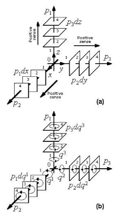
Figure 1: Basis vectors and one-forms in Euclidean $\mathbb{R}^{3}-$space: (a) Translational case; and (b) Rotational case [21]. For the same geometry in $\mathbb{R}^{3}$, see [35].

• any scalar function $f=f(x,y,z)$ is a 0–form;

• the gradient $\mathbf{d}f=\mathbf{\omega}$ of any smooth function $f$ is a 1–form

  $$\mathbf{\omega=d}f=\frac{\partial f}{\partial x}dx+\frac{\partial f}{\partial y}dy+\frac{\partial f}{\partial z}dz;$$

• the curl $\mathbf{\alpha=d\omega}$ of any smooth 1–form $\mathbf{\omega}$ is a 2–form

  $$\mathbf{\alpha=d\omega}=\left(\frac{\partial R}{\partial y}-\frac{\partial Q}{\partial z}\right)dydz+\left(\frac{\partial P}{\partial z}-\frac{\partial R}{\partial x}\right)dzdx+\left(\frac{\partial Q}{\partial x}-\frac{\partial P}{\partial y}\right)dxdy;$$

  $$\text{if }\mathbf{\omega=d}f\Rightarrow\mathbf{\alpha=dd}f=0.$$

• the divergence $\mathbf{\beta=d\alpha}$ of any smooth 2–form $\mathbf{\alpha}$ is a 3–form

  $$\mathbf{\beta=d\alpha}=\left(\frac{\partial A}{\partial x}+\frac{\partial B}{\partial y}+\frac{\partial C}{\partial z}\right)dxdydz;\qquad\text{if }\mathbf{\alpha=d\omega}\Rightarrow\mathbf{\beta=dd\omega}=0.$$

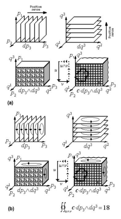
Figure 2: Fundamental two–form and its flux in $\mathbb{R}^{3}$: (a) Translational case; (b) Rotational case. In both cases the flux through the plane $u\wedge v$ is defined as $\int\int_{u\wedge v}c\,dp_{i}dq^{i}$ and measured by the number of tubes crossed by the circulation oriented by $u\wedge v$ [21]. For the same geometry in $\mathbb{R}^{3}$, see [35].

In general, for any two smooth functions $f=f(x,y,z)$ and $g=g(x,y,z)$, the exterior derivative $\mathbf{d}$ obeys the Leibniz rule [23, 24]:

$$\mathbf{d}(fg)=g\,\mathbf{d}f+f\,\mathbf{d}g,$$

and the chain rule:

$$\mathbf{d}\left(g(f)\right)=g^{\prime}(f)\,\mathbf{d}f.$$

2.3 Exterior $p-$forms in $\mathbb{R}^{4}$

In general, given a so–called 4D coframe, that is a set of coordinate differentials $\{dx^{i}\}\in\mathbb{R}^{4}$, we can define the space of all $p-$forms, denoted $\Omega^{p}(\mathbb{R}^{4})$, using the exterior derivative $\mathbf{d}:\Omega^{p}(\mathbb{R}^{4})\rightarrow\Omega^{p+1}(\mathbb{R}^{4})$ and Einstein’s summation convention over repeated indices (e.g., $A_{i}\,dx^{i}=\sum_{i=0}^{3}A_{i}\,dx^{i}$), we have:

1–form

– a generalization of the Green’s 1–form $Pdx+Qdy$,

$$\mathbf{A}=A_{i}\,dx^{i}\in\Omega^{1}(\mathbb{R}^{4}).$$

For example, in 4D electrodynamics, $\mathbf{A}$ represents electromagnetic (co)vector potential.

2–form

– generalizing the Green’s 2–form $(\partial_{x}Q-\partial_{y}P)\,dxdy$  $($with $\partial_{j}=\partial/\partial x^{j}$),

$$\mathbf{B} = \mathbf{dA}\in\Omega^{2}(\mathbb{R}^{4}),\qquad\text{with components}$$

$$\mathbf{B} = \frac{1}{2}B_{ij}\,dx^{i}\wedge dx^{j},\qquad\text{or}$$

$$\mathbf{B} = \partial_{j}A_{i}\,dx^{j}\wedge dx^{i},\qquad\text{so that}$$

$$B_{ij} = -2\partial_{j}A_{i}=\partial_{i}A_{j}-\partial_{j}A_{i}=-B_{ji}.$$

where $\wedge$ is the anticommutative exterior (or, ‘wedge’) product of two differential forms; given a $p-$form $\mathbf{\alpha}\in\Omega^{p}(\mathbb{R}^{4})$ and a $q-$form $\mathbf{\beta}\in\Omega^{q}(\mathbb{R}^{4}),$ their exterior product is a $(p+q)-$form $\mathbf{\alpha}\wedge\mathbf{\beta}\in\Omega^{p+q}(\mathbb{R}^{4})$; e.g., if we have two 1–forms $\mathbf{a}=a_{i}dx^{i}$, and $\mathbf{b}=b_{i}dx^{i}$, their wedge product $\mathbf{a}\wedge\mathbf{b}$ is a 2–form $\mathbf{\alpha}$ given by

$$\mathbf{\alpha}=\mathbf{a}\wedge\mathbf{b}=a_{i}b_{j}\,dx^{i}\wedge dx^{j}=-a_{i}b_{j}\,dx^{j}\wedge dx^{i}=-\mathbf{b}\wedge\mathbf{a}.$$

The exterior product $\wedge$ is related to the exterior derivative $\mathbf{d}$, by

$$\mathbf{d}(\mathbf{\alpha}\wedge\mathbf{\beta})=\mathbf{d\alpha}\wedge\mathbf{\beta}+(-1)^{p}\mathbf{\alpha}\wedge\mathbf{d\beta}.\text{ \ }$$

3–form

$$\mathbf{C} = \mathbf{dB~{}(}=\mathbf{ddA}\equiv 0)\in\Omega^{3}(\mathbb{R}^{4}),\qquad\text{with components}$$

$$\mathbf{C} = \frac{1}{3!}C_{ijk}\,dx^{i}\wedge dx^{j}\wedge dx^{k},\qquad\text{or}$$

$$\mathbf{C} = \partial_{k}B_{[ij]}\,dx^{k}\wedge dx^{i}\wedge dx^{j},\qquad\text{so that}$$

$$C_{ijk} = -6\partial_{k}B_{[ij]},\qquad\text{where }B_{[ij]}\text{ is the skew--symmetric part of }B_{ij}.$$

For example, in the 4D electrodynamics, $\mathbf{B}$ represents the field 2–form Faraday, or the Liénard–Wiechert 2–form (in the next section we will use the standard symbol $\mathbf{F}$ instead of $\mathbf{B}$) satisfying the sourceless magnetic Maxwell’s equation,

$$\text{Bianchi identity}:\quad\mathbf{dB}=0,\quad\text{in components\quad}\partial_{k}B_{[ij]}=0.$$

4–form

$$\mathbf{D} = \mathbf{dC~{}(}=\mathbf{ddB}\equiv 0)\in\Omega^{4}(\mathbb{R}^{4}),\qquad\text{with components}$$

$$\mathbf{D} = \partial_{l}C_{[ijk]}\,dx^{l}\wedge dx^{i}\wedge dx^{j}\wedge dx^{k},\qquad\text{or}$$

$$\mathbf{D} = \frac{1}{4!}D_{ijkl}\,dx^{i}\wedge dx^{j}\wedge dx^{k}\wedge dx^{l},\qquad\text{so that}$$

$$D_{ijkl} = -24\partial_{l}C_{[ijk]}.$$

2.4 Stokes Theorem in $\mathbb{R}^{4}$

Generalization of the Green’s theorem in the plane (and all other integral theorems from vector calculus) is the Stokes Theorem for the $p-$form $\mathbf{\omega}$, in the $n$D domain $C$ (which is a $p-$chain with a $(p-1)-$boundary $\partial C$, see next subsection)

$$\int_{\partial C}\mathbf{\omega}=\int_{C}\mathbf{d\omega}.$$

In the 4D Euclidean space $\mathbb{R}^{4}$ we have the following three particular cases of the Stokes theorem, related to the subspaces $C$ of $\mathbb{R}^{4}$:

The 2D Stokes theorem:

$$\int_{\partial C^{2}}\mathbf{A}=\int_{C^{2}}\mathbf{B}.$$

The 3D Stokes theorem:

$$\int_{\partial C^{3}}\mathbf{B}=\int_{C^{3}}\mathbf{C}.$$

The 4D Stokes theorem:

$$\int_{\partial C^{4}}\mathbf{C}=\int_{C^{4}}\mathbf{D}.$$

2.5 Exact and closed $p-$forms and $p-$chains

Notation: we drop boldface letters from now on. In general, a $p-$form $\beta$ is called closed if its exterior derivative is equal to zero,

$$d\beta=0.$$

From this condition one can see that the closed form (the kernel of the exterior derivative operator $d$) is conserved quantity. Therefore, closed $p-$forms possess certain invariant properties, physically corresponding to the conservation laws (see e.g., [30]).

Also, a $p-$form $\beta$ that is an exterior derivative of some $(p-1)-$form $\alpha$,

$$\beta=d\alpha,$$

is called exact (the image of the exterior derivative operator $d$). By Poincaré Lemma, exact forms prove to be closed automatically,

$$d\beta=d(d\alpha)=0.$$

Since $d^{2}=0$, every exact form is closed. The converse is only partially true (Poincaré Lemma): every closed form is locally exact. This means that given a closed $p-$form on a smooth manifold $M$ (see Appendix), $\alpha\in\Omega^{p}(M)$ on an open set $U\subset M$, any point $m\in U$ has a neighborhood on which there exists a $(pk-1)-$form $\beta\in\Omega^{p-1}(U)$ such that $d\beta=\alpha|_{U}.$

The Poincaré lemma is a generalization and unification of two well–known facts in vector calculus:
(i) If $\mathop{\mathrm{c}url}F=0$, then locally $F=\mathop{\mathrm{g}rad}f$;   and   (ii) If $\mathop{\mathrm{d}iv}F=0$, then locally $F=\mathop{\mathrm{c}url}G$.

Poincaré lemma for contractible manifolds: Any closed form on a smoothly contractible manifold is exact.

A cycle is a chain $C\in\mathcal{C}_{p}(M)$ such that $\partial C=0$. A boundary is a chain $C$ such that $C=\partial B,$ for any other chain $B\in\mathcal{C}_{p}(M)$. Similarly, a cocycle (i.e., a closed form) is a cochain $\omega$ such that $d\omega=0$. A coboundary (i.e., an exact form) is a cochain $\omega$ such that $\omega=d\theta,$ for any other cochain $\theta$. All exact forms are closed ($\omega=d\theta\Rightarrow d\omega=0$) and all boundaries are cycles ($C=\partial B\Rightarrow\partial C=0$). Converse is true only for smooth contractible manifolds, by Poincaré Lemma.

2.6 Topological duality of $p-$forms and $p-$chains

Duality of $p-$forms and $p-$chains on a smooth manifold $M$ is based on the

$$\text{Period:}\ \ \int_{C}\omega:=\left\langle C,\omega\right\rangle,$$

where $C$ is a cycle, $\omega$ is a cocycle, while $\left\langle C,\omega\right\rangle=\omega(C)$ is their inner product $\left\langle C,\omega\right\rangle:\Omega^{p}(M)\times\mathcal{C}_{p}(M)\rightarrow\mathbb{R}$, a bilinear non-degenerate functional (pairing) on $M$ [31]. From Poincaré Lemma, a closed $p-$form $\omega$ is exact iff $\left\langle C,\omega\right\rangle=0$.

The fundamental topological duality is based on the Stokes theorem,

$$\int_{\partial C}\omega=\int_{C}d\omega\qquad\mathrm{or}\qquad\left\langle\partial C,\omega\right\rangle=\left\langle C,d\omega\right\rangle,$$

where $\partial C$ is the boundary of the $p-$chain $C$ oriented coherently with $C$ on $M$. While the boundary operator $\partial$ is a global operator, the coboundary operator $d$ is local, and thus more suitable for applications. The main property of the exterior differential,

$$d\circ d\equiv d^{2}=0\quad\Longrightarrow\quad\partial\circ\partial\equiv\partial^{2}=0,\qquad(\text{and converse}),$$

can be easily proved using the Stokes’ theorem as

$$0=\left\langle\partial^{2}C,\omega\right\rangle=\left\langle\partial C,d\omega\right\rangle=\left\langle C,d^{2}\omega\right\rangle=0.$$

2.7 The de Rham cochain complex

In the Euclidean 3D space $\mathbb{R}^{3}$ we have the following de Rham cochain complex

$$0\rightarrow\Omega^{0}(\mathbb{R}^{3})\underset{\mathrm{grad}}{\stackrel{{\scriptstyle d}}{{\longrightarrow}}}\Omega^{1}(\mathbb{R}^{3})\underset{\mathrm{curl}}{\stackrel{{\scriptstyle d}}{{\longrightarrow}}}\Omega^{2}(\mathbb{R}^{3})\underset{\mathrm{div}}{\stackrel{{\scriptstyle d}}{{\longrightarrow}}}\Omega^{3}(\mathbb{R}^{3})\rightarrow 0.$$

Using the closure property for the exterior differential in $\mathbb{R}^{3},~{}d\circ d\equiv d^{2}=0$, we get the standard identities from vector calculus

$$\mathop{\mathrm{c}url}\cdot\mathop{\mathrm{g}rad}=0\text{ \ \ \ \ \ \ and \ \ \ \ \ \ }\mathop{\mathrm{d}iv}\cdot\mathop{\mathrm{c}url}=0.$$

As a duality, in $\mathbb{R}^{3}$ we have the following chain complex

$$0\leftarrow\mathcal{C}_{0}(\mathbb{R}^{3}){\stackrel{{\scriptstyle\partial}}{{\longleftarrow}}}\mathcal{C}_{1}(\mathbb{R}^{3}){\stackrel{{\scriptstyle\partial}}{{\longleftarrow}}}\mathcal{C}_{2}(\mathbb{R}^{3}){\stackrel{{\scriptstyle\partial}}{{\longleftarrow}}}\mathcal{C}_{3}(\mathbb{R}^{3})\leftarrow 0,$$

(with the closure property $\partial\circ\partial\equiv\partial^{2}=0$) which implies the following three boundaries:

$$C_{1}\stackrel{{\scriptstyle\partial}}{{\mapsto}}C_{0}=\partial(C_{1}),\qquad C_{2}\stackrel{{\scriptstyle\partial}}{{\mapsto}}C_{1}=\partial(C_{2}),\qquad C_{3}\stackrel{{\scriptstyle\partial}}{{\mapsto}}C_{2}=\partial(C_{3}),$$

where $C_{0}\in{\cal C}_{0}$ is a 0–boundary (or, a point), $C_{1}\in{\cal C}_{1}$ is a 1–boundary (or, a line), $C_{2}\in{\cal C}_{2}$ is a 2–boundary (or, a surface), and $C_{3}\in{\cal C}_{3}$ is a 3–boundary (or, a hypersurface). Similarly, the de Rham complex implies the following three coboundaries:

$$C^{0}\stackrel{{\scriptstyle d}}{{\mapsto}}C^{1}=d(C^{0}),\qquad C^{1}\stackrel{{\scriptstyle d}}{{\mapsto}}C^{2}=d(C^{1}),\qquad C^{2}\stackrel{{\scriptstyle d}}{{\mapsto}}C^{3}=d(C^{2}),$$

where $C^{0}\in\Omega^{0}$ is 0–form (or, a function), $C^{1}\in\Omega^{1}$ is a 1–form, $C^{2}\in\Omega^{2}$ is a 2–form, and $C^{3}\in\Omega^{3}$ is a 3–form.

In general, on a smooth $n$D manifold $M$ we have the following de Rham cochain complex [33]

$$0\rightarrow\Omega^{0}(M)\overset{d}{\longrightarrow}\Omega^{1}(M)\overset{d}{\longrightarrow}\Omega^{2}(M)\overset{d}{\longrightarrow}\Omega^{3}(M)\overset{d}{\longrightarrow}\cdot\cdot\cdot\overset{d}{\longrightarrow}\Omega^{n}(M)\rightarrow 0,$$

satisfying the closure property on $M,~{}d\circ d\equiv d^{2}=0$.

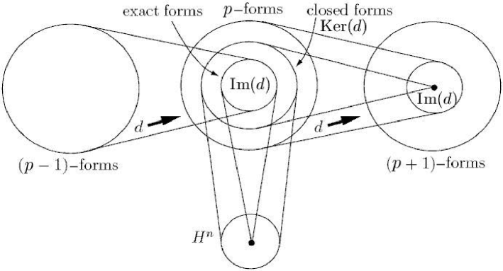
Figure 3: A small portion of the de Rham cochain complex, showing a homomorphism of cohomology groups.

2.8 (Co)homology on a smooth manifold $M$

The subspace of all closed $p-$forms (cocycles) on a smooth manifold $M$ is the kernel $\mathop{\mathrm{K}er}(d)$ of the de Rham $d-$homomorphism (see Figure 3), denoted by $Z^{p}(M)\subset\Omega^{p}(M)$, and the sub-subspace of all exact $p-$forms (coboundaries) on $M$ is the image $\mathop{\mathrm{I}m}(d)$ of the de Rham homomorphism denoted by $B^{p}(M)\subset Z^{p}(M)$. The quotient space

$$H^{p}(M):=\frac{Z^{p}(M)}{B^{p}{M}}=\frac{\mathop{\mathrm{K}er}\left(d:\Omega^{p}(M)\rightarrow\Omega^{p+1}(M)\right)}{\mathop{\mathrm{I}m}\left(d:\Omega^{p-1}(M)\rightarrow\Omega^{p}(M)\right)},$$

is called the $p$th cohomology group of a manifold $M$. It is a topological invariant of a manifold. Two $p-$cocycles $\alpha$,$\beta\in\Omega^{p}(M)$ are homologous, or belong to the same cohomology class $[\alpha]\in H^{p}(M)$, if they differ by a $(p-1)-$coboundary $\alpha-\beta=d\theta\in\Omega^{p-1}(M)$.

Similarly, the subspace of all $p-$cycles on a smooth manifold $M$ is the kernel $\mathop{\mathrm{K}er}(\partial)$ of the $\partial-$homomorphism, denoted by $Z_{p}(M)\subset\mathcal{C}_{p}(M)$, and the sub-subspace of all $p-$boundaries on $M$ is the image $\mathop{\mathrm{I}m}(\partial)$ of the $\partial-$homomorphism, denoted by $B_{p}(M)\subset\mathcal{C}_{p}(M)$. Two $p-$cycles $C_{1}$,$C_{2}\in\mathcal{C}_{p}$ are homologous, if they differ by a $(p-1)-$boundary $C_{1}-C_{2}=\partial B\in\mathcal{C}_{p-1}(M)$. Then $C_{1}$ and $C_{2}$ belong to the same homology class $[C]\in H_{p}(M)$, which is defined as

$$H_{p}(M):=\frac{Z_{p}(M)}{B_{p}(M)}=\frac{\mathop{\mathrm{K}er}(\partial:\mathcal{C}_{p}(M)\rightarrow\mathcal{C}_{p-1}(M))}{\mathop{\mathrm{I}m}(\partial:\mathcal{C}_{p+1}(M)\rightarrow\mathcal{C}_{p}(M))},$$

where $Z_{p}$ is the vector space of cycles and $B_{p}\subset Z_{p}$ is the vector space of boundaries on $M$.

2.9 A cochain complex spanning the space-time manifold

Consider a small portion of the de Rham cochain complex of Figure 3 spanning a space-time 4–manifold $M$,

$$\Omega^{p-1}(M)\overset{d_{p-1}}{\longrightarrow}\Omega^{p}(M)\overset{d_{p}}{\longrightarrow}\Omega^{p+1}(M)$$

As we have seen above, cohomology classifies topological spaces by comparing two subspaces of  $\Omega^{p}$:  (i) the space of $p-$cocycles, $Z^{p}(M):=\mathop{\mathrm{K}er}d_{p}$, and  (ii) the space of $p-$coboundaries, $B^{p}(M):=\mathop{\mathrm{I}m}d_{p-1}$. Thus, for the cochain complex of any space-time 4–manifold we have,

$$d^{2}=0\quad\Longrightarrow\quad B^{p}(M)\subset Z^{p}(M),$$

that is, every $p-$coboundary is a $p-$cocycle. Whether the converse of this statement is true, according to Poincaré Lemma, depends on the particular topology of a space-time 4–manifold. If every $p-$cocycle is a $p-$coboundary, so that $B^{p}$ and $Z^{p}$ are equal, then the cochain complex is exact at $\Omega^{p}(M)$. In topologically interesting regions of a space-time manifld $M$, exactness may fail, and we measure the failure of exactness by taking the $p$th cohomology group

$$H^{p}(M):=Z^{p}(M)/B^{p}(M).$$

2.10 Hodge star, codifferential and Laplacian

The Hodge star operator $\star:\Omega^{p}(M)\rightarrow\Omega^{n-p}(M)$ on a smooth manifold $M$ is defined as [32]

$$\alpha\wedge\star\,\beta=\beta\wedge\star\,\alpha=\left\langle\alpha,\beta\right\rangle\mu,\qquad\text{for }\alpha,\beta\in\Omega^{p}(M).$$

The $\star$ operator depends on the Riemannian metric on $M$ and also on the orientation (reversing orientation will change the sign). The volume form $\mu$ is defined in local coordinates on $M$ as

$$\mu=\text{vol}=\star(1)=\sqrt{\det(g_{ij})}~{}dx^{1}\wedge...\wedge dx^{n},$$

and the total volume on $M$ is given by

$$\mathop{\mathrm{v}ol}(M)=\int_{M}\star(1).$$

For example, in the 4D electrodynamics, the dual 2–form Maxwell $\star F$ satisfies the electric Maxwell equation with the source [35],

$$\text{Dual Bianchi identity}:\quad\mathbf{d}\mathbf{\star F}=\mathbf{\star J},$$

where $\mathbf{\star J}$ is the 3–form dual to the charge–current 1–form $\mathbf{J}$.

For any to $p-$forms $\alpha,\beta\in\Omega^{p}(M)$ with compact support, we define the (bilinear and positive–definite) Hodge $L^{2}-$inner product as

$$(\alpha,\beta)=\int_{M}\langle\alpha,\beta\rangle\star(1)=\int_{M}\alpha\wedge\star\beta.$$ (2)

We can extend the product $(\cdot,\cdot)$ to $L^{2}(\Omega^{p}(M))$; it remains bilinear and positive–definite, because as usual in the definition of $L^{2}$, functions that differ only on a set of measure zero are identified.

Now, the Hodge dual to the exterior derivative $d:\Omega^{p}(M)\rightarrow\Omega^{p+1}(M)$ on a smooth manifold $M$ is the codifferential $\delta$, a linear map $\delta:\Omega^{p}(M)\rightarrow\Omega^{p-1}(M)$, which is a generalization of the divergence, defined by [32]

$$\delta=\star\,d\star(-1)^{n(p+1)+1},\qquad\text{so that\qquad}d=\star\,\delta\star(-1)^{np}.$$

Applied to any $p-$form $\omega\in\Omega^{p}(M)$, the codifferential $\delta$ gives

$$\delta\omega=(-1)^{n(p+1)+1}\star d\star\omega.$$

If $\omega=f$ is a $0-$form, or function, then $\delta f=0$.

The codifferential $\delta$ can be coupled with the exterior derivative $d$ to construct the Hodge Laplacian $\Delta:$ $\Omega^{p}(M)\rightarrow\Omega^{p}(M),$ a harmonic generalization of the Laplace–Beltrami differential operator, given by

$$\Delta=\delta d+d\delta.$$

The Hodge codifferential $\delta$ satisfies the following set of rules:

• $\delta\delta=\delta^{2}=0,$  the same as $\ dd=d^{2}=0;$

• $\delta\Delta=\Delta\delta,$  the same as $\ d\Delta=\Delta d;$

• $\delta\star=(-1)^{p+1}\star d$;  $\star\,\delta=(-1)^{p}\star d$;

• $d\delta\star=\star\,\delta d$;  $\star\,d\delta=\delta d\star$;  $\star\,\Delta=\Delta\star.$

3 Classical Gauge Electrodynamics in 4D

Recall that a gauge theory is a theory that admits a symmetry with a local parameter. For example, in every quantum theory the global phase of the wave $\psi-$function is arbitrary and does not represent something physical. Consequently, the theory is invariant under a global change of phases (adding a constant to the phase of all wave functions, everywhere); this is a global symmetry. In quantum electrodynamics, the theory is also invariant under a local change of phase, that is, one may shift the phase of all wave functions so that the shift may be different at every point in space-time. This is a local symmetry. However, in order for a well–defined derivative operator to exist, one must introduce a new field, the gauge field, which also transforms in order for the local change of variables (the phase in our example) not to affect the derivative. In quantum electrodynamics this gauge field is the electromagnetic potential 1–form $A$, in components given by

$$A=A_{\mu}dx^{\mu},\quad\text{such that}\quad A_{\mathrm{new}}=A_{\mathrm{old}}+df,$$

(where $f$ is an arbitrary scalar function) – leaves the electromagnetic field 2–form $F=dA$ unchanged. This change $df$ of local gauge of variable $A$ is termed gauge transformation. In quantum field theory the excitations of fields represent particles. The particle associated with excitations of the gauge field is the gauge boson. All the fundamental interactions in nature are described by gauge theories. In particular, in quantum electrodynamics, whose gauge transformation is a local change of phase, the gauge group is the circle group $U(1)$ (consisting of all complex numbers with absolute value $1$), and the gauge boson is the photon (see e.g., [37]).

In the 4D space-time electrodynamics, the 1–form electric current density $J$ has the components $J_{\mu}=(\rho,\mathbf{j})=(\rho,j_{x},j_{y},j_{z})$ (where $\rho$ is the charge density), the 2–form Faraday $F$ is given in components of electric field $\mathbf{E}$ and magnetic field $\mathbf{B}$ by

$$F_{\mu\nu}=\left(\begin{array}[]{cccc}0&E_{x}&E_{y}&E_{z}\\ -E_{x}&0&-B_{z}&B_{y}\\ -E_{y}&B_{z}&0&-B_{x}\\ -E_{z}&-B_{y}&B_{x}&0\end{array}\right),\qquad\text{with\qquad}F_{\nu\mu}=-F_{\mu\nu}$$

while its dual 2–form Maxwell $\star F$ has the following components

$$\star F_{\mu\nu}=\left(\begin{array}[]{cccc}0&-B_{x}&-B_{y}&-B_{z}\\ B_{x}&0&-E_{z}&E_{y}\\ B_{y}&E_{z}&0&-E_{x}\\ B_{z}&-E_{y}&B_{x}&0\end{array}\right),\qquad\text{with\qquad}\star F_{\nu\mu}=-\star F_{\mu\nu}.$$

3.1 Maxwell’s equations

The gauge field in classical electrodynamics, in local coordinates given as an electromagnetic potential 1–form

$$A=A_{\mu}dx^{\mu}=A_{\mu}dx^{\mu}+df,\qquad(f=~{}\text{arbitrary scalar field}),$$

is globally a connection on a $U(1)-$bundle (see Appendix). The corresponding electromagnetic field, locally the 2–form

$$F = dA,\qquad\text{in components given by}$$

$$F = \frac{1}{2}F_{\mu\nu}\,dx^{\mu}\wedge dx^{\nu},\qquad\text{with \ \ \ }F_{\mu\nu}=\partial_{\nu}A_{\mu}-\partial_{\mu}A_{\nu}$$

is globally the curvature of the connection $A$ under the gauge–covariant derivative,

$$D_{\mu}=\partial_{\mu}-{\mathrm{i}}eA_{\mu},$$

where ${\mathrm{i}}=\sqrt{-1}$ and $e$ is the charge coupling constant.

Classical electrodynamics is governed by the Maxwell equations, which in exterior formulation read

$$dF = 0,\qquad\delta F=-4\pi J,\qquad\text{or in components,}$$

$$F_{[\mu\nu,\eta]} = 0,\qquad F_{\mu\nu},^{\mu}=-4\pi J_{\mu},$$

where comma denotes the partial derivative and the 1–form of electric current $J=J_{\mu}dx^{\mu}$ is conserved, by the electrical continuity equation,

$$\delta J=0,\qquad\text{or in components,\qquad}J_{\mu},^{\mu}=0.$$

The first, sourceless Maxwell equation, $dF=0$, gives vector magnetostatics and magnetodynamics,

Magnetic Gauss’ law $$: \mathop{\mathrm{d}iv}\mathbf{B}=0,\qquad$$

Faraday’s law : $$\partial_{t}\mathbf{B}+\mathop{\mathrm{c}url}\mathbf{E}=0.$$

The second Maxwell equation with source, $\delta F=J$, gives vector electrostatics and electrodynamics,

Electric Gauss’ law $$: \mathop{\mathrm{d}iv}\mathbf{E}=4\pi\rho,\qquad$$

Ampère’s law $$: \partial_{t}\mathbf{E}-\mathop{\mathrm{c}url}\mathbf{B}=-4\pi\mathbf{j}.$$

Maxwell’s equations are generally applied to macroscopic averages of the fields, which vary wildly on a microscopic scale in the vicinity of individual atoms, where they undergo quantum effects as well (see below).

3.2 Electrodynamic action

The standard Lagrangian for the free electromagnetic field, $F=dA$, is given by [23, 24, 25]

$$\mathcal{L}(A)=\frac{1}{2}(F\wedge\star\,F),$$

with the corresponding action

$$S(A)=\frac{1}{2}\int F\wedge\star\,F.$$

Using the Hodge $L^{2}-$inner product (2), we can rewrite this action as

$$S(A)=\frac{1}{2}(F,F).$$ (3)

3.3 2D electrodynamics

One of the reasons that gauge electrodynamics in 2D is especially simple is that the electromagnetic field $F=dA$, being a 2–form, can be written simply as a scalar field $\varphi=\varphi(x,t)$ times the volume form [44]

$$F=\varphi\;\mathrm{vol}.$$

This means that the only Hodge duals we need to consider are the trivial ones,

$$\star~{}\mathrm{vol}=1\qquad~{}\text{and}\qquad\star 1=\mathrm{vol},$$

so the 2D Lagrangian for vacuum electrodynamics is given by [43]

$$L=\frac{1}{2}(\varphi\;\mathrm{vol})\wedge\star\,(\varphi\;\mathrm{vol})=\frac{1}{2}\varphi^{2}\;\mathrm{vol}\wedge 1=\frac{\varphi^{2}}{2}\mathrm{vol}.$$

4 Quantum Electrodynamics in 4D

Quantum electrodynamics (QED) is a relativistic quantum field theory of electrodynamics. QED was developed by four Nobel Laureates, P. Dirac, R. Feynman, J. Schwinger and S. Tomonaga, and F. Dyson, between 1920s and 1950s. It describes some aspects of how electrons, positrons and photons interact. QED mathematically describes all phenomena involving electrically charged particles interacting by means of exchange of photons.

4.1 Dirac QED

The Dirac equation for a particle with mass $m$ (in natural units) reads (see, e.g., [25])

$$({\mathrm{i}}\gamma^{\mu}\partial_{\mu}-m)\psi=0,\qquad(\mu=0,1,2,3)$$ (4)

where ${\mathrm{i}}=\sqrt{-1}$ $\psi(x)$ is a 4–component spinor wave–function, the so–called Dirac spinor, while $\gamma^{\mu}$ are $4\times 4$ Dirac $\gamma-$matrices,

$$\gamma^{0}=\begin{pmatrix}1&0&0&0\\ 0&1&0&0\\ 0&0&-1&0\\ 0&0&0&-1\end{pmatrix},\qquad \gamma^{1}\!=\!\begin{pmatrix}0&0&0&1\\ 0&0&1&0\\ 0&-1&0&0\\ -1&0&0&0\end{pmatrix},$$

$$\gamma^{2}\!=\!\begin{pmatrix}0&0&0&-i\\ 0&0&i&0\\ 0&i&0&0\\ -i&0&0&0\end{pmatrix},\qquad \gamma^{3}\!=\!\begin{pmatrix}0&0&1&0\\ 0&0&0&-1\\ -1&0&0&0\\ 0&1&0&0\end{pmatrix}.$$

They obey the anticommutation relations

$$\{\gamma^{\mu},\gamma^{\nu}\}=\gamma^{\mu}\gamma^{\nu}+\gamma^{\nu}\gamma^{\mu}=2g^{\mu\nu},$$

where $g_{\mu\nu}$ is the metric tensor.

Dirac’s $\gamma-$matrices are conventionally derived as

$$\gamma^{k}=\begin{pmatrix}0&\sigma^{k}\\ -\sigma^{k}&0\end{pmatrix},\qquad(k=1,2,3)$$

where $\sigma^{k}$ are Pauli $\sigma-$matrices (a set of $2\times 2$ complex Hermitian and unitary matrices), defined as

$$\sigma_{1}=\sigma_{x}=\begin{pmatrix}0&1\\ 1&0\end{pmatrix},\qquad\sigma_{2}=\sigma_{y}=\begin{pmatrix}0&-i\\ i&0\end{pmatrix},\qquad\sigma_{3}=\sigma_{z}=\begin{pmatrix}1&0\\ 0&-1\end{pmatrix},$$

obeying both the commutation and anticommutation relations

$$[\sigma_{i},\sigma_{j}]=2i\,\varepsilon_{ijk}\,\sigma_{k},\qquad\{\sigma_{i},\sigma_{j}\}=2\delta_{ij}\cdot I,$$

where $\varepsilon_{ijk}$ is the Levi–Civita symbol, $\delta_{ij}$ is the Kronecker delta, and $I$ is the identity matrix.

Now, the Lorentz–invariant form of the Dirac equation (4) for an electron with a charge $e$ and mass $m_{\mathrm{e}}$, moving with a 4–momentum 1–form $p=p_{\mu}dx^{\mu}$ in a classical electromagnetic field defined by 1–form $A=A_{\mu}dx^{\mu}$, reads (see, e.g., [39, 25]):

$$\left\{{\mathrm{i}}\gamma^{\mu}\left[p_{\mu}-eA_{\mu}\right]-m_{\mathrm{e}}\right\}\psi(x)=0,$$ (5)

and is called the covariant Dirac equation.

The formal QED Lagrangian (density) includes three terms,

$$\mathcal{L}(x)=\mathcal{L}_{\mathrm{em}}(x)+\mathcal{L}_{\mathrm{int}}(x)+\mathcal{L}_{\mathrm{e-p}}(x),$$ (6)

related respectively to the free electromagnetic field 2–form $F=F_{\mu\nu}dx^{\mu}\wedge dx^{\nu}$, the electron–positron field (in the presence of the external vector potential 1–form $A_{\mu}^{\mathrm{ext}})$, and the interaction field (dependent on the charge–current 1–form $J=J_{\mu}dx^{\mu}$). The free electromagnetic field Lagrangian in (6) has the standard electrodynamic form

$$\mathcal{L}_{\mathrm{em}}(x)=-\frac{1}{4}F^{\mu\nu}F_{\mu\nu},$$

where the electromagnetic fields are expressible in terms of components of the potential 1–form
$A=A_{\mu}dx^{\mu}$ by

$$F_{\mu\nu}=\partial_{\mu}A_{\nu}^{\mathrm{tot}}-\partial_{\nu}A_{\mu}^{\mathrm{tot}},\quad\text{with\quad}A_{\mu}^{\mathrm{tot}}=A_{\mu}^{\mathrm{ext}}+A_{\mu}.$$

The electron-positron field Lagrangian is given by Dirac’s equation (5) as

$$\mathcal{L}_{\mathrm{e-p}}(x)=\bar{\psi}(x)\left\{{\mathrm{i}}\gamma^{\mu}\left[p_{\mu}-eA_{\mu}^{\mathrm{ext}}\right]-m_{\mathrm{e}}\right\}\psi(x),$$

where $\bar{\psi}(x)$ is the Dirac adjoint spinor wave function.

The interaction field Lagrangian

$$\mathcal{L}_{\mathrm{int}}(x)=-J^{\mu}A_{\mu},$$

accounts for the interaction between the uncoupled electrons and the radiation field.

The field equations deduced from (6) read

$$\left\{{\mathrm{i}}\gamma^{\mu}\left[p_{\mu}-eA_{\mu}^{\mathrm{ext}}\right]-m_{\mathrm{e}}\right\}\psi(x) = \gamma^{\mu}\psi(x)A_{\mu},$$

$$\partial^{\mu}F_{\mu\nu} = J_{\nu}.$$ (7)

The formal QED requires the solution of the system (7) when $A^{\mu}(x),$ $\psi(x)$ and $\bar{\psi}(x)$ are quantized fields.

4.2 Feynman QED

In Feynman’s form of quantum electrodynamics [40, 24, 25], the process of quantization is transparent – it is performed using his path integral formalism, resulting in the quantum–field transition given (in natural units) by:

$$\langle out_{A}A|in_{A}\rangle=\int\mathcal{D}[A]\,{\mathrm{e}}^{{\mathrm{i}}S(A)}\quad\underrightarrow{Wick}\quad\int\mathcal{D}[A]\,{\mathrm{e}}^{-S(A)},\qquad$$ (8)

with action $S(A)$ given by (13) in the exponent (multiplied by the imaginary unit i). The Lebesgue integration in (8) is performed over electromagnetic fields $A_{\mu}$, with the Lebesgue measure

$$\mathcal{D}[A]=\lim_{N\allowbreak\mathrel{\mathop{\hbox to8.4pt{\rightarrowfill}}\limits}\infty}\prod_{s=1}^{N}dA^{s}_{\mu}\qquad(\mu=1,..,4).$$

The transformation $\underrightarrow{Wick}$ denotes the so–called Wick–rotation of the time variable $t$ to imaginary values $t\mapsto\tau={\mathrm{i}}t$, thereby transforming the complex-valued path integral into the real-valued (Euclidean) one. The absolute square of the transition amplitude (8) gives the transition probability density function, $P(A)=|\langle out_{A}|in_{A}\rangle|^{2}$. Full discretization of (8) ultimately gives the standard thermodynamic partition function

$$Z=\sum_{j}{\mathrm{e}}^{-E^{j}/T},$$ (9)

where $E^{j}$ is the energy eigenvalue, $T$ is the temperature environmental control parameter, and the sum runs over all $j$ energy eigenstates. From (9), we can further calculate all thermodynamical and statistical properties [41], as for example, transition entropy $S=k_{B}\ln Z$, etc.

The standard QED considers the path integral

$$Z[A] = \int\mathcal{D}[A]\,\mathrm{e}^{\mathrm{i}S[A]},\qquad\text{where the action for the free e.-m. field is}$$

$$S[A] = \int d^{4}x\left[-\frac{1}{4}(F_{\mu\nu})^{2}\right]=\frac{1}{2}\int d^{4}x\,A_{\mu}(x)\left(\partial^{2}g^{\mu\nu}-\partial^{\mu}\partial^{\nu}\right)A_{\nu}(x).$$

$Z[A]$ is the path integral over each of the four spacetime components:

$$\mathcal{D}[A]=\mathcal{D}[A]^{0}\mathcal{D}[A]^{1}\mathcal{D}[A]^{2}\mathcal{D}[A]^{3}.$$

This functional integral is badly divergent, due to gauge invariance. Recall that $F_{\mu\nu},$ and hence $L,$ is invariant under a general gauge transformation of the form

$$A_{\mu}(x)\rightarrow A_{\mu}(x)+\frac{1}{e}\partial_{\mu}\alpha(x).$$

The troublesome modes are those for which  $A_{\mu}(x)=\partial_{\mu}\alpha(x),$ that is, those that are gauge–equivalent to  $A_{\mu}(x)=0.$ The path integral is badly defined because we are redundantly integrating over a continuous infinity of physically equivalent field configurations. To fix this problem, we would like to isolate the interesting part of the path integral, which counts each physical configuration only once. This can be accomplished using the Faddeev–Popov trick [42], which effectively adds a term to the system Lagrangian and after which we get

$$Z[A]=\int\mathcal{D}[A]\exp\left[\mathrm{i}\int_{-T}^{T}d^{4}x\,\left[\mathcal{L}-\frac{1}{2\xi}(\partial^{\mu}A_{\mu})^{2}\right]\right],$$

where $\xi$ is any finite constant.

Now, the observable $O$ in the quantum field theory is a real–valued function of the gauge field: $O\colon\mathcal{A}\rightarrow\mathbb{R},$ where $\mathcal{A}$ is the space of connections, so we can try to calculate its expected value using the electrodynamic action $S(A)$ (13) as

$$\left\langle\Omega|T\,\mathcal{O}(A)|\Omega\right\rangle=\frac{\int_{\mathcal{A}}\mathcal{D}[A]O(A)\,\mathrm{e}^{-S(A)}}{\int_{\mathcal{A}}\mathcal{D}[A]\,\mathrm{e}^{-S(A)}}.$$

In certain cases, it might be difficult to define exactly what this means. Even in the finite dimensional case, where $\mathcal{D}[A]$ is the Lebesgue measure on $\mathcal{A}$, when we try to calculate $\langle O\rangle$ by the above formula we usually run into serious problems. To see this, let us do a sample calculation of the integral in the denominator, which is the partition function

$$Z:=\int_{\mathcal{A}}\mathcal{D}[A]\,\mathrm{e}^{-S(A)}$$ (10)

against which all other expected values are normalized.

Thus, the Faddeev–Popov trick needs also to be applied to the formula for the two–point correlation function

$$\left\langle\Omega|T\,\mathcal{O}(A)|\Omega\right\rangle=\lim_{T\rightarrow\infty(1-i\epsilon)}\frac{\int\mathcal{D}[A]\,\mathcal{O}(A)\exp\left[\mathrm{i}\int_{-T}^{T}d^{4}x\,\mathcal{L}\right]\mathcal{\,}}{\int\mathcal{D}[A]\exp\left[\mathrm{i}\int_{-T}^{T}d^{4}x\,\mathcal{L}\right]},$$

which after Faddeev–Popov procedure becomes

$$\left\langle\Omega|T\,\mathcal{O}(A)|\Omega\right\rangle=\lim_{T\rightarrow\infty(1-i\epsilon)}\frac{\int\mathcal{D}[A]\,\mathcal{O}(A)\exp\left[\mathrm{i}\int_{-T}^{T}d^{4}x\,\left[\mathcal{L}-\frac{1}{2\xi}(\partial^{\mu}A_{\mu})^{2}\right]\right]\mathcal{\,}}{\int\mathcal{D}[A]\exp\left[\mathrm{i}\int_{-T}^{T}d^{4}x\,\left[\mathcal{L}-\frac{1}{2\xi}(\partial^{\mu}A_{\mu})^{2}\right]\right]}.$$

The space of gauge transformations, $\mathcal{G}$, is a group which acts on the space $\mathcal{A}$ of connections by

$$\mathcal{G}\times\mathcal{A}\rightarrow\mathcal{A},\qquad(\phi,A)\mapsto A+d\phi.$$

A common way of eliminating divergences caused by gauge freedom is gauge fixing [43], which means choosing some method to pick one representative of each gauge–equivalence class $[A]$ and doing path integrals over these. There are problems with this approach, however. In a general gauge theory, it might not even be possible to fix a smooth, global gauge over which to integrate. But even when we can do this, the arbitrary choice involved in fixing a gauge is undesirable, philosophically. Gauge fixing amounts to pretending a quotient space of $\mathcal{A}$, the space of connections modulo gauge transformations, is a subspace. A better approach is to use the quotient space directly. Namely, modding out by the action of $\mathcal{G}$ on $\mathcal{A}$ gives the quotient space $\mathcal{A/G}$ consisting of gauge–equivalence classes of connections, and we do path integrals like

$$Z=\int_{\mathcal{A}/\mathcal{G}}d[A]\,\mathrm{e}^{-S([A])}.$$

When gauge fixing works, path integrals over $\mathcal{A/G}$ give the same results as gauge fixing. But integrating over $\mathcal{A/G}$ is more general and involves no arbitrary choices.

Since gauge equivalent connections are regarded as physically equivalent, the quotient space ${\mathcal{A}/\mathcal{G}}$ of connections mod gauge transformations is sometimes called the physical configuration space for vacuum electrodynamics. A physical observable is then any real–valued function on the physical configuration space, $O:{\mathcal{A}/\mathcal{G}}\rightarrow\mathbb{R},$ or equivalently, any gauge–invariant function on the space $\mathcal{A}$ of connections. In the case of noncompact gauge group even factoring out all of the gauge freedom may be insufficient to regularize our path integrals. In particular, there are certain topological conditions our space-time must meet for this programme to give convergent path integrals. As a consequence, in the case where the gauge group is $\mathbb{R}$, we must sometimes take more drastic measures in order to extract meaningful results, and this leads to some interesting differences between the cases $G=\mathbb{R}$ and $G=U(1)$ as the gauge group for electrodynamics. These differences are related to the famous ‘Bohm–Aharonov effect’ [43].

4.3 Cohomology criterion for path–integral convergence

To eliminate the divergences in the path integral (10) it is necessary that we eliminate any gauge freedom from the space of connections $\mathcal{A}$. In gauge theory, the action $S(A)$ is invariant under the group of gauge transformations $\mathcal{G}$. In case of a gauge group $\mathcal{G}=\mathbb{R}$, we have gauge transformations of the form

$$A\mapsto A+d\varphi,$$

where $\varphi$ is an arbitrary $(p-1)-$cochain. In other words, two $p-$connections are gauge equivalent if they differ by a $p-$coboundary $d\varphi\in B^{p}$. Before we saw that the existence of gauge freedom implied path integrals such as the one above must diverge [43]. The standard procedure of eliminating any gauge freedom from the space of connections $\mathcal{A}$ is to pass to the quotient space

$$\mathcal{A}/\mathcal{G}=C^{p}/B^{p},$$

that is, $p-$connections modulo gauge transformations, effectively declaring gauge equivalent $p-$connections to be equal. In particuclar, the criterion in $\mathbb{R}$ electrodynamics for path integrals over the physical configuration space $\mathcal{A/G}$ to converge is that the first cohomology be trivial [43]:

$$\left(\begin{array}[]{c}Z=\int_{\mathcal{A/G}}\mathcal{D}[A]\,\mathrm{e}^{-S(A)}\\ \text{converges for $\mathbb{R}$ electrodynamics}\end{array}\right)\iff H^{1}=0.$$

5 Electro–Muscular Stimulation

In this section we develop covariant biophysics of electro–muscular stimulation, as an externally induced generator of the covariant muscular force,

$$F_{i}=m_{ij}\,a^{i},$$ (11)

where $F_{i}$ are covariant components of the muscular force (torque) 1–form $F=F_{i}(t)\,dx^{i}$, $m_{ij}$ are the covariant components of the musculo-skeletal metric/inertia tensor $m=m_{ij}\;dx^{i}\otimes dx^{j}$, while $a^{i}=a^{i}(t)\,\partial_{x^{i}}$ are contravariant components of the angular acceleration vector (see [22, 23] for technical details). The so–called functional electrical stimulation (FES) of human skeletal muscles is used in rehabilitation and in medical orthotics to externally stimulate the muscles with damaged neural control. However, the repetitive use of electro–muscular stimulation, besides functional, causes also structural changes in the stimulated muscles, giving the physiological effect of muscular training.

The use of low and very low frequency impulses in the body, delivered through electrodes, is known as transcutaneous stimulation of the nerves, electro–acupuncture and electro–stimulation. Here, an electromagnetic field accompanies the passage of the electric current through the conductive wire. This is generally known as the term ‘electromagnetic therapy’.

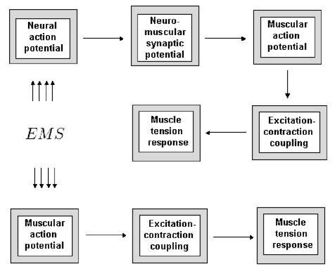
Figure 4: Schematic of electro–muscular stimulation ($EMS$).

In particular, electro–muscular stimulation ($EMS$, see Figure 4) represents a union of external electrical stimulation fields, internal myofibrillar excitation–contraction paths, and dissipative skin & fat geometries, formally given by

$$EMS=EMS_{fields}\bigcup EMS_{paths}\bigcup EMS_{geom}.$$ (12)

In Feynman’s QED formulation, corresponding to each of the three $EMS$–phases in (12) we formulate:

1. The least action principle, to model a unique, external–anatomical, predictive and smooth, macroscopic $EMS$ field–path–geometry; and

2. Associated Feynman path integral, to model an ensemble of rapidly and stochastically fluctuating, internal, microscopic, fields–paths–geometries of the cellular $EMS$, to which the external–anatomical macro–level represents both time and ensemble average.

In the proposed formalism, muscular excitation–contraction paths $x^{i}(t)$ are caused by electromagnetic stimulation fields $\Phi^{k}=\Phi^{k}(t,x,y,z)$, by the the Lorenz force equation (1), while they are both affected by dissipative and noisy skin & fat shapes and curvatures, defined by the local Riemannian musculo-skeletal metric tensor $m_{ij}$ (11). In particular, the electromagnetic 2–form Faraday $F=F_{\alpha\beta}\,dx_{\alpha}dx_{\beta}$, defines the Lorentz force 1–form $Q=Q_{\alpha}\,dx_{\alpha}$ of the electro–muscular stimulation,

$$Q_{\alpha}\equiv\dot{p}_{\alpha}\propto qF_{\alpha\beta}v^{\beta},$$

where $q$ is total electric charge and $v^{\beta}$ is the velocity vector–field of the stimulation flow. This equation says that the muscular force 1–form $Q_{\alpha}$ generated by the simulation is proportional to the stimulation field strength $F_{\alpha\beta}$, velocity of the stimulation flow $v^{\beta}$ through the skin–fat–muscle tissue, as well as the total stimulation charge $q$.

In the following text, we first formulate the global model for the $EMS$, to set up the general formalism to be specialized subsequently for each of the three $EMS$–phases.

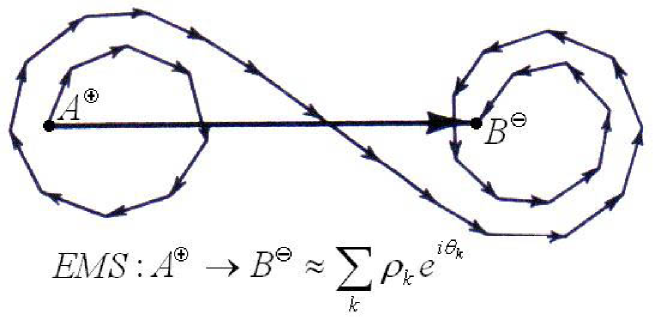
Figure 5: Simplified Feynman–like experimental approach to electrical muscular stimulation: the flow of electric current from the positive surface pad $A^{\oplus}$ to the negative pad $B^{\ominus}$ can be approximated by the vector sum of complex vectors $\rho_{k}\,{\mathrm{e}}^{i\theta_{k}}$, where $\theta_{k}$ are proportional to the time taken by each vector $\rho_{k}$; this vector sum will be further developed into Feynman integral.

5.1 Global macro $EMS-$level

In general, at the macroscopic $EMS$–level we first formulate the total action $S[\Phi]$, our central quantity, which can be described through physical dimensions of $Energy\times Time=Effort$, which is also the dimension of the Planck constant $\hbar$ ($=1$ in normal units). This total action quantity has immediate biophysical ramifications: the greater the action – the higher the stimulation effect on the new shape. The action $S[\Phi]$ depends on macroscopic fields, paths and geometries, commonly denoted by an abstract field symbol $\Phi^{i}$. The action $S[\Phi]$ is formally defined as a temporal integral from the initial time instant $t_{ini}$ to the final time instant $t_{fin}$,

$$S[\Phi]=\int_{t_{ini}}^{t_{fin}}\mathfrak{L}[\Phi]\,dt,$$ (13)

with Lagrangian density, given by

$$\mathfrak{L}[\Phi]=\int d^{n}x\,\mathcal{L}(\Phi^{i},\partial_{x^{j}}\Phi^{i}),$$

where the integral is taken over all $n$ coordinates $x^{j}=x^{j}(t)$ of the $EMS$, and $\partial_{x^{j}}\Phi^{i}$ are time and space partial derivatives of the $\Phi^{i}-$variables over coordinates.

Second, we formulate the least action principle as a minimal variation $\delta$ of the action $S[\Phi]$

$$\delta S[\Phi]=0,$$ (14)

which, using variational Euler–Lagrangian equations, derives field–motion–geometry of the unique and smooth $EMS-$transition map (or, more appropriately, ‘functor’ [24])

$$\mathcal{T}:STIMUL_{t_{ini}}\Rightarrow CONTRACT_{t_{mid}}\Rightarrow SHAPE_{t_{fin}},$$

acting at a macro–level from some initial time $t_{ini}$ to the final time $t_{fin}$ (via the intermediate time $t_{mid}$).

In this way, we get macro–objects in the global $EMS$: a single electrodynamic stimulation field described by Maxwell field equations, a single muscular excitation–contraction path described by Lagrangian equation of motion, and a single Riemannian skin & fat geometry.

5.2 Local Micro $EMS-$level

After having properly defined macro–level $EMS$, we move down to the microscopic cellular $EMS$–level of rapidly fluctuating electrodynamic fields, sarcomere–contraction paths and coarse–grained, fractal muscle–fat geometry, where we cannot define a unique and smooth field–path–geometry. The most we can do at this level of fluctuating noisy uncertainty, is to formulate an adaptive path integral and calculate overall probability amplitudes for ensembles of local transitions from negative $EMS$–pad $A^{\ominus}$ to the positive pad $B^{\oplus}$ (see Figure 5). This probabilistic transition micro–dynamics is given by a multi field–path–geometry, defining the microscopic transition amplitude corresponding to the macroscopic $EMS-$transition map $\mathcal{T}$. So, what is externally the transition map, internally is the transition amplitude. The absolute square of the transition amplitude is the transition probability.

Now, the total $EMS-$transition amplitude, from the initial state $STIMUL$, to the final state $SHAPE$, is defined on $EMS$

$$\langle SHAPE|STIMUL\rangle:STIMUL_{t_{0}}\Rrightarrow SHAPE_{t_{1}},$$ (15)

given by modern adaptive generalization of the Feynman’s path integral, see [25]). The transition map (15) calculates overall probability amplitude along a multitude of wildly fluctuating fields, paths and geometries, performing the microscopic transition from the micro–state $STIMUL_{t_{0}}$ occurring at initial micro–time instant $t_{0}$ to the micro–state $SHAPE_{t_{1}}$ at some later micro–time instant $t_{1}$, such that all micro–time instants fit inside the global transition interval $t_{0},t_{1},...,t_{s}\in[t_{ini},t_{fin}]$. It is symbolically written as

$$\langle SHAPE|STIMUL\rangle=\int\mathcal{D}[w\Phi]\,{\mathrm{e}}^{\mathrm{i}S[\Phi]},$$ (16)

where the Lebesgue integration is performed over all continuous $\Phi^{i}_{con}=fields+paths+geometries$, while summation is performed over all discrete processes and regional topologies $\Phi^{j}_{dis}$. The symbolic differential $\mathcal{D}[w\Phi]$ in the general path integral (16), represents an adaptive path measure, defined as a weighted product

$$\mathcal{D}[w\Phi]=\lim_{N\allowbreak\mathrel{\mathop{\hbox to8.4pt{\rightarrowfill}}\limits}\infty}\prod_{s=1}^{N}w_{s}d\Phi_{s}^{i},\qquad({i=1,...,n=con+dis}),$$ (17)

which is in practice satisfied with a large $N$.

In this way, we get a range of micro–objects in the local $EMS$ at the short time–level: ensembles of rapidly fluctuating, noisy and crossing electrical stimulation fields, myofibrillar contraction paths and local skin & fat shape–geometries. However, by averaging process, both in time and along ensembles of fields, paths and geometries, we can recover the corresponding global, smooth and fully predictive, external $EMS$ transition–dynamics $\mathcal{T}$.

5.3 Micro–Level Adaptation and Muscular Training

The adaptive path integral (16–17) incorporates the local muscular training process according to the basic learning formula

$$NEW\,\,VALUE=OLD\,\,VALUE+INNOVATION,$$

where the term $VALUE$ represents respectively biological images of the $STIMUL$,
$CONTRACT$ and $SHAPE$.

The general synaptic weights $w_{s}=w_{s}(t)$ in (17) are updated by the homeostatic neuro–muscular feedbacks during the transition process $\mathcal{T}$, according to one of the two standard neural training schemes, in which the micro–time level is traversed in discrete steps, i.e., if $t=t_{0},t_{1},...,t_{s}$ then $t+1=t_{1},t_{2},...,t_{s+1}$:

1. A self–organized, unsupervised, e.g., Hebbian–like training rule (see, e.g. [28]:

   $$w_{s}(t+1)=w_{s}(t)+\frac{\sigma}{\eta}(w_{s}^{d}(t)-w_{s}^{a}(t)),$$ (18)

   where $\sigma=\sigma(t),\,\eta=\eta(t)$ denote signal and noise, respectively, while superscripts $d$ and $a$ denote desired and achieved muscular micro–states, respectively; or

2. A certain form of a supervised gradient descent training:

   $$w_{s}(t+1)\,=\,w_{s}(t)-\eta\nabla J(t),$$ (19)

   where $\eta$ is a small constant, called the step size, or the training rate, and $\nabla J(n)$ denotes the gradient of the ‘performance hyper–surface’ at the $t-$th iteration.

For more details EMS–fields, paths and geometries, see [25].

6 Appendix: Manifolds and Bundles

6.1 Manifolds

Smooth manifold is a curved $n$D space which is locally equivalent to $\mathbb{R}^{n}$. To sketch it formal definition, consider a set $M$ (see Figure 6) which is a candidate for a manifold. Any point $x\in M$ has its Euclidean chart, given by a 1–1 and onto map $\varphi_{i}:M\rightarrow\mathbb{R}^{n}$, with its Euclidean image $V_{i}=\varphi_{i}(U_{i})$. More precisely, a chart $\varphi_{i}$ is defined by

$$\varphi_{i}:M\supset U_{i}\ni x\mapsto\varphi_{i}(x)\in V_{i}\subset\mathbb{R}^{n},$$

where $U_{i}\subset M$ and $V_{i}\subset\mathbb{R}^{n}$ are open sets.

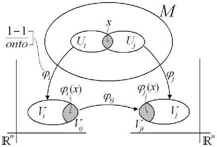
Figure 6: Geometric picture of the manifold concept.

Clearly, any point $x\in M$ can have several different charts (see Figure 6). Consider a case of two charts, $\varphi_{i},\varphi_{j}:M\rightarrow\mathbb{R}^{n}$, having in their images two open sets, $V_{ij}=\varphi_{i}(U_{i}\cap U_{j})$ and $V_{ji}=\varphi_{j}(U_{i}\cap U_{j})$. Then we have transition functions $\varphi_{ij}$ between them,

$$\varphi_{ij}=\varphi_{j}\circ\varphi_{i}^{-1}:V_{ij}\rightarrow V_{ji},\qquad\text{locally given by\qquad}\varphi_{ij}(x)=\varphi_{j}(\varphi_{i}^{-1}(x)).$$

If transition functions $\varphi_{ij}$ exist, then we say that two charts, $\varphi_{i}$ and $\varphi_{j}$ are compatible. Transition functions represent a general (nonlinear) transformations of coordinates, which are the core of classical tensor calculus.

A set of compatible charts $\varphi_{i}:M\rightarrow\mathbb{R}^{n},$ such that each point $x\in M$ has its Euclidean image in at least one chart, is called an atlas. Two atlases are equivalent iff all their charts are compatible (i.e., transition functions exist between them), so their union is also an atlas. A manifold structure is a class of equivalent atlases.

Finally, as charts $\varphi_{i}:M\rightarrow\mathbb{R}^{n}$ were supposed to be 1-1 and onto maps, they can be either homeomorphisms, in which case we have a topological ($C^{0}$) manifold, or diffeomorphisms, in which case we have a smooth ($C^{k}$) manifold.

6.2 Fibre Bundles

On the other hand, the well–known tangent bundle $TM$ and cotangent bundle $T^{\ast}M$ of a smooth manifold $M$, respectively endowed with Riemannian geometry (suitable for Lagrangian dynamics) and symplectic geometry (suitable for Hamiltonian dynamics) – are special cases of a more general geometrical object called fibre bundle. Here the word fiber $V$ of a map $\pi:Y\rightarrow X$ denotes the preimage $\pi^{-1}(x)$ of an element $x\in X$. It is a space which locally looks like a product of two spaces (similarly as a manifold locally looks like Euclidean space), but may possess a different global structure. To get a visual intuition behind this fundamental geometrical concept, we can say that a fibre bundle $Y$ is a homeomorphic generalization of a product space $X\times V$ (see Figure 7), where $X$ and $V$ are called the base and the fibre, respectively. $\pi:Y\rightarrow X$ is called the projection, $Y_{x}=\pi^{-1}(x)$ denotes a fibre over a point $x$ of the base $X$, while the map $f=\pi^{-1}:X\rightarrow Y$ defines the cross–section, producing the graph $(x,f(x))$ in the bundle $Y$ (e.g., in case of a tangent bundle, $f=\dot{x}$ represents a velocity vector–field, so that the graph in a the bundle $Y$ reads $(x,\dot{x})$).

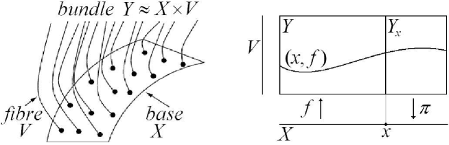
Figure 7: A sketch of a fibre bundle $Y\approx X\times V$ as a generalization of a product space $X\times V$; left – main components; right – a few details (see text for explanation).

The main reason why we need to study fibre bundles is that all dynamical objects (including vectors, tensors, differential forms and gauge potentials) are their cross–sections, representing generalizations of graphs of continuous functions.

References

- [1] Brazier, M.A.B. A History of the Electrical Activity of the Brain. Pitman, London, (1961).
- [2] Hodgkin, A.L., Huxley, A.F., Katz, B. Measurements of current-voltage relations in the membrane of the giant axon of Loligo. J. Physiol. 116: 424 448, (1952).
- [3] Hodgkin, A.L., Huxley, A.F. Currents carried by sodium and potassium ions through the membrane of the giant axon of Loligo. J. Physiol. 116:449 472, (1952).
- [4] Hodgkin, A.L., Huxley, A.F. The components of membrane conductance in the giant axon of Loligo. J. Physiol. 116:473 496, (1952).
- [5] Hodgkin, A.L., Huxley, A.F. The dual effect of membrane potential on sodium conductance in the giant axon of Loligo. J. Physiol. 116: 497 506, (1952).
- [6] Hodgkin, A.L., Huxley, A.F. A quantitative description of membrane current and its application to conduction and excitation in nerve. J. Physiol. 117: 500 544, (1952).
- [7] Rall, W. Cable Theory for Dendritic Neurons, in C. Koch and I. Segev: Methods in Neuronal Modeling: From Synapses to Networks. Cambridge MA: Bradford Books, MIT Press, pp. 9 62, (1989).
- [8] Hodgkin, A.L., Rushton, W.A.H. The electrical constants of a crustacean nerve fibre. Proc. Roy. Soc. B 133: 444 79, (1946).
- [9] Noble, D. Cardiac action and pacemaker potentials based on the Hodgkin-Huxley equations. Nature 188: 495 497, (1960).
- [10] Kléber, A.G., Rudy, Y. Basic mechanisms of cardiac impulse propagation and associated arrhythmias. Physiol. Rev. 84 (2): 431 88, (2004).
- [11] Epstein, C.M. Introduction to EEG and evoked potentials. J.B. Lippincot Co. (1983).
- [12] Braunwald, E. (ed), Heart Disease: A Textbook of Cardiovascular Medicine, (5th ed), Saunders, Philadelphia, (1997).
- [13] Mark, J.B. Atlas of cardiovascular monitoring. Churchill Livingstone, New York, (1998).
- [14] Cram, J.R., Kasman, G.S., Holtz, J., Introduction to Surface Electromyography. Aspen Publishers Inc., Gaithersburg, Maryland, (1998).
- [15] Reaz, M.B.I., Hussain, M.S., Mohd-Yasin, F., Techniques of EMG Signal Analysis: Detection, Processing, Classification and Applications, Biological Procedures Online, vol. 8, issue 1, pp. 11-35, (2006).
- [16] D.O. Carpenter, S. Ayrapetyan, Biological Effects of Electric and Magnetic Fields, (Volumes 1 & 2), Academic Press, New York, (1994).
- [17] E. Valentini, G. Curcio, F. Moroni, M. Ferrara, L. De Gennaro, M. Bertini, Neurophysiological Effects of Mobile Phone Electromagnetic Fields on Humans: A Comprehensive Review, Bioelectromagnetics 28:415 432, (2007).
- [18] J.M. Elwood, Epidemiological Studies of Radio Frequency Exposures and Human Cancer, Bioelectromagnetics Supplement 6:S63 S73, (2003).
- [19] G. Vincze, A. Szasz, A.R. Liboff, New Theoretical Treatment of Ion Resonance Phenomena, Bioelectromagnetics 29:380 386, (2008).
- [20] J.E. Marsden, A. Tromba, Vector Calculus (5th ed.), W. Freeman and Company, New York, (2003)
- [21] V. Ivancevic, Symplectic Rotational Geometry in Human Biomechanics, SIAM Rev. 46, 3, 455–474, (2004).
- [22] V. Ivancevic, T. Ivancevic, Human–Like Biomechanics. Springer, Dordrecht, (2006).
- [23] V. Ivancevic, T. Ivancevic, Geometrical Dynamics of Complex Systems. Springer, Dordrecht, (2006).
- [24] V. Ivancevic, T. Ivancevic, Applied Differfential Geometry: A Modern Introduction. World Scientific, Singapore, (2007)
- [25] V. Ivancevic, T. Ivancevic, Quantum Leap: From Dirac and Feynman, Across the Universe, to Human Body and Mind. World Scientific, Singapore, (2008)
- [26] V. Ivancevic, T. Ivancevic, High–Dimensional Chaotic and Attractor Systems. Springer, Berlin, (2006).
- [27] V. Ivancevic, T. Ivancevic, Natural Biodynamics. World Scientific, Singapore, (2006)
- [28] V. Ivancevic, T. Ivancevic, Neuro-Fuzzy Associative Machinery for Comprehensive Brain and Cognition Modelling. Springer, Berlin, (2007)
- [29] V. Ivancevic, T. Ivancevic, Computational Mind: A Complex Dynamics Perspective. Springer, Berlin, (2007)
- [30] Abraham, R., Marsden, J., Ratiu, T., Manifolds, Tensor Analysis and Applications. Springer, New York, (1988).
- [31] Choquet-Bruhat, Y., DeWitt-Morete, C., Analysis, Manifolds and Physics (2nd ed). North-Holland, Amsterdam, (1982).
- [32] Voisin, C., Hodge Theory and Complex Algebraic Geometry I. Cambridge Univ. Press, Cambridge, (2002).
- [33] De Rham, G., Differentiable Manifolds. Springer, Berlin, (1984).
- [34] Flanders, H., Differential Forms: with Applications to the Physical Sciences. Acad. Press, (1963).
- [35] C.W. Misner, K.S. Thorne, J.A. Wheeler, Gravitation. W. Freeman and Company, New York, (1973).
- [36] I. Ciufolini, J.A. Wheeler, Gravitation and Inertia, Princeton Series in Physics, Princeton University Press, Princeton, New Jersey, (1995).
- [37] P.H. Frampton, Gauge Field Theories, Frontiers in Physics. Addison-Wesley, (1986).
- [38] J.C. Baez, J.P. Muniain, Gauge Fields, Knots and Gravity, Series on Knots and Everything – Vol. 4. World Scientific, Singapore, (1994).
- [39] Drake, G.W.F (ed.), Springer Handbook of Atomic, Molecular, and Optical Physics. Springer, New York, (2006)
- [40] R.P. Feynman, Quantum Electrodynamics. Advanced Book Classics, Perseus Publishing, (1998).
- [41] R.P. Feynman, Statistical Mechanics, A Set of Lectures. WA Benjamin, Inc., Reading, Massachusetts, (1972).
- [42] L.D. Faddeev and V.N. Popov, Feynman diagrams for the Yang–Mills field. Phys. Lett. B 25, 29, (1967).
- [43] D.K. Wise, p-form electrodynamics on discrete spacetimes. Class. Quantum Grav. 23, 5129–5176, (2006).
- [44] E. Witten, On quantum gauge theories in two dimensions, Commun. Math. Phys. 141, 153–209, (1991).