Network Topology as a Driver of Bistability in the lac Operon

Abstract.

The lac operon in Escherichia coli has been studied extensively and is one of the earliest gene systems found to undergo both positive and negative control. The lac operon is known to exhibit bistability, in the sense that the operon is either induced or uninduced. Many dynamical models have been proposed to capture this phenomenon. While most are based on complex mathematical formulations, it has been suggested that for other gene systems network topology is sufficient to produce the desired dynamical behavior.

We present a Boolean network as a discrete model for the lac operon. We include the two main glucose control mechanisms of catabolite repression and inducer exclusion in the model and show that it exhibits bistability. Further we present a reduced model which shows that lac mRNA and lactose form the core of the lac operon, and that this reduced model also exhibits the same dynamics. This work corroborates the claim that the key to dynamical properties is the topology of the network and signs of interactions.

1. Introduction

The lac operon in the bacterium Escherichia coli has been used as a model system of gene regulation since the landmark work by Jacob and Monod in 1961 [6]. Its study has led to numerous insights into sugar metabolism, including how the presence of a substrate could trigger induction of its catabolizing enzyme, yet in the presence of a preferred energy source, namely glucose, the substrate is rendered ineffective. Originally termed the “glucose effect”, catabolite repression became known as one of the mechanisms by which glucose regulates the induction of sugar-metabolizing operons. Early work on the lac operon also led to the discovery that transcription of an operon’s genes is subject to positive or negative control and that the system of genes is either inducible (inducers are needed to kick-start transcription) or repressible (corepressors are needed to stop transcription). The lac operon is one of the earliest examples of a inducible system of genes being under both positive and negative control.

There are many formulations modeling the behavior and interaction of the lac genes. The first model was proposed by Goodwin two years after the discovery of the lac operon  [3]. Since then there has been a steady flow of models following the advances in biological insight of the system, with the majority describing operon induction using artificial nonmetabolizable compounds such as IPTG and TMG [10, 16, 17, 13]. For example, the first model to consider catabolite repression and inducer exclusion, another control mechanism of the operon by glucose, when the cells were grown in both glucose and lactose (lactose was the inducer) was presented by Wong et al. [18]. Their model consisted of up to 13 ordinary differential equations involving 65 parameters. Further Santillán and coauthors have presented mathematical models and analysis purporting bistability (the operon is either induced or uninduced) [19, 12, 13, 11] as observed in the experiments of [9, 10]. These findings have given rise to the analogy of the lac operon acting as a biological switch [10, 5].

Most mathematical formulations of the lac operon, as well as other genetic systems, are given as systems of differential equations; however, discrete modeling frameworks are receiving more attention for their use in offering global insights. In fact Albert and Othmer suggested that network topology and the type of interactions, as opposed to quantitative mathematical functions with estimated parameters, were sufficient to capture the dynamics of gene networks, which they demonstrated by constructing a Boolean model for a segment polarity network in Drosophila melanogaster [2]. Setty et al. defined a logical function for the transcription of the lac genes in terms of the proteins regulating the operon, namely CRP and LacI [14]. Although the authors initially aimed to construct a simple Boolean function to mimic the switching behavior of the operon, they discovered that AND-like and OR-like expressions could not reproduce the complexity that the lac genes exhibited. Instead they found that a logical function on 4 states (as opposed to 2 states - 0 and 1) was more biologically relevant. Mayo et al. tested and showed that this logical function was robust with respect to point mutations, that is, given the formulation in [14], the operon is still functional after point mutations [8].

To our knowledge, the model of Setty et al. is the first discrete model of the lac genes. While this is an important example of the applicability of logical functions for describing operon dynamics, one limitation is that it does not predict bistability. We propose a logical model for the lac operon which predicts bistability (when stochasticity is included) and includes the two main control mechanisms of glucose, namely catabolite repression and inducer exclusion. In order to facilitate interpretation, we have added variables so as to present the model as a Boolean network. Advantages of a Boolean framework are that it naturally encodes network topology and interaction type by way of Boolean expressions and it permits an intuitive, yet formal mathematical description, a feature that is not readily accessible for more general logical models. An advantage of discrete models in general is that the entire state space can be computed and explored, in contrast to continuous modeling frameworks. Therefore we are able to show that the lac operon has only two steady states, corresponding to the operon being either ON or OFF (induced or uninduced).

An important question is to identify the key players in a network, in this case for the purpose of determining the drivers of the dynamics. Aguda and Goryachev provided a systematic approach for reducing a network pieced together from literature to a subnetwork which can be thought of as the core of the essential qualitative behavior [1]. Albert and Othmer [2] showed that the topology and interaction type are the determining factors in producing the steady-state behavior. We corroborate these findings by reducing the Boolean model to a one involving only the lac genes and lactose. We show that the dynamics of the reduced model matches that of the full model. Our results further support the hypothesis that the topology is the key to dynamical properties.

The paper is organized as follows. In Section 2 we present the biological and modeling background; we also present a Boolean network as a model for the lac operon. We present its network topology, associated dynamics and bistability experiments. Section 3 contains the reduction steps and the reduced model. We close with a discussion of future work in Section 4.

2. Model

2.1. Biological Background

Here we describe the components and features of the lac operon which we include in the model. This description is summarized largely from the material provided in the online book [4]. Additional citations are given as necessary.

The lac operon contains three structural genes, lacZ, lacY, and lacA, and is a negative inducible system: the repressor protein LacI prevents transcription of the lac genes, and the operon is induced by allolactose, an isomer of lactose. Extracellular lactose is thought to be readily available, but can diffuse into the cell at low concentrations. Once in the cell, lactose can induce the operon, though with lower probability than allolactose. Transcription of the lac genes gives rise to a single mRNA, whose translation gives rise to the following proteins: $\beta$-galactoside permease (LacY), a membrane-bound protein which transports lactose into the cell; $\beta$-galactosidase (LacZ), an intracellular protein which cleaves lactose into glucose and its stereoisomer galactose, and which converts lactose into allolactose; and $\beta$-galactoside transacetylase (LacA) which transfers an acetyl group from acetyl-CoA to $\beta$-galactosides.

Glucose is thought to regulate the lac operon through two key mechanisms: catabolite repression and inducer exclusion. In the absence of glucose, the catabolite activator protein CAP (also known as CRP for cAMP receptor protein) forms a complex with cAMP which binds to a site upstream of the lac promoter region. Binding of the cAMP-CAP complex makes a conformational change in the DNA, thereby allowing RNA polymerase to bind to the DNA and enhancing transcription of the lac genes. Transcription continues until extracellular glucose is available. However, when glucose is abundant, cAMP synthesis is inhibited [18] and the repressor protein LacI can bind to the operator region of the operon, preventing transcription of the lac genes. The presence of (sufficient amounts of) glucose shuts off the operon, a phenomenon referred to as catabolite repression. The second mechanism, inducer exclusion, occurs when the transport of lactose into the cell by permease is inhibited by external glucose.

2.2. Modeling Background

A Boolean network on $n$ variables is a collection of functions (defined over the set {0,1}) $f_{1},\ldots,f_{n}$ such that for each $i=1,\ldots,n$, the function $f_{i}$ determines the next state of variable $i$ and is written in terms of the Boolean operators $\vee,\wedge,\neg$ (logical OR, AND, and NOT, respectively). The values 0 and 1 are the states of the variables.

“Network topology” refers to the connectivity structure of a network and is typically represented as a directed graph. For a Boolean network, a wiring diagram is a directed graph on the variables of the system (in this case, mRNA, proteins, and sugars) with edges defined in the following way: there is a directed edge from variable $x_{i}$ to $x_{j}$ if the function $f_{x_{j}}$ for $x_{j}$ depends on $x_{i}$. An edge from $x_{i}$ to $x_{j}$ has a small circle at its head $x_{j}$ if $\neg x_{i}$ appears in $f_{x_{j}}$ (we consider this edge to correspond to an inhibitory interaction); otherwise, edges have arrows at their heads. We call directed cycles feedback loops. The parity of a feedback loop (or a path) can be either +1 or -1 and is calculated as follows. Assign -1 to an edge if it is inhibitory and +1 otherwise. The parity of a feedback loop is the product of +1/-1 on the edges of the loop. If the parity of a feedback loop is +1, we call the loop positive; otherwise, it is negative.

“Dynamics” refers to the state transitions of the network as a whole. To generate the dynamics of a Boolean network $F$ on $n$ variables, we evaluate its functions on all possible combinations of 0-1 $n$-tuples. The dynamics can be viewed as a directed graph, called the state space of $F$. In this graph each node is a state ($n$-tuple) of the system; there is a directed edge from $a$ to $b$ if $F$ evaluated at the current state $a$ gives state $b$; that is, if $F(a)=b$. Hence, $b$ represents that next state of the system. Directed cycles are called limit cycles. If length of the cycle is 1, then it is called a fixed point. In the context of scientific applications, fixed points are also referred to as steady states, which we use in this discourse. We draw the state space using the visualization software DVD [7].

2.3. Boolean Network

In this subsection we present the Boolean network for the lac operon that models gene regulation such as the two main control mechanisms of glucose, namely catabolite repression and inducer exclusion. The Boolean network consists of variables and functions, each representing mRNAs, proteins and sugars. We assume that each biomolecule can be either 0 or 1 (absent/inactive or present/active). The Boolean variables are labeled as follows:

• $M$ = lac mRNA

• $P,B$ = lac permease and $\beta$-galactosidase, resp.

• $C$ = catabolite activator protein CAP

• $R$ = repressor protein LacI

• $L$, $A$= lactose and allolactose (inducer), resp.

• $L_{l}$, $A_{l}$ = (at least) low concentration of lactose and allolactose, resp.

Next we derive the Boolean functions for mRNA based on the information in Section 2.1. The other Boolean functions are constructed in a similar fashion (see Supporting Information).

Boolean function for $M$: When the concentration of the repressor is high ($R=1$), the production of mRNA will be low ($M=0$) independent of the concentration of CAP ($C$). On the other hand, when the concentration of the repressor is low ($G=0$) and the concentration of CAP is high ($C=1$), mRNA production will be high ($M=1$). In other words, $M$ will be 1 when $R$ is not 1 and $C$ is 1; that is, the future Boolean value of $M$ is NOT $R$ AND $C$. Hence, the Boolean function for $M$ is $H_{M}=\neg R\wedge C$.

The complete Boolean network is given as follows ($\wedge$, $\vee$ and $\neg$ are the logical AND, OR and NOT operators, respectively):

$$\begin{array}[]{ll}H_{M}=\neg R\wedge C&\\ H_{P}=M&H_{B}=M\\ H_{C}=\neg G_{e}&H_{R}=\neg A\wedge\neg A_{l}\\ H_{A}=L\wedge B&H_{A_{l}}=A\vee L\vee L_{l}\\ H_{L}=\neg G_{e}\wedge P\wedge L_{e}&H_{L_{l}}=\neg G_{e}\wedge(L\vee L_{e})\\ \end{array}$$

where $L_{e}$, $G_{e}$ represent extracellular lactose and glucose, respectively, and are considered as parameters in the model. For any variable $a$, the function $H_{a}$ determines the value of $a$ after one time unit. We use $H$ to refer to the model consisting of this Boolean network.

2.3.1. Network Topology

The network topology for the model $H$ is shown in Figure 1 and is displayed as a wiring diagram (see Section 2.2 for definitions). From the diagram we can identify topological features such as the feedback loops in $H$. We see that there are at least two positive feedback loops involving $M$, namely $M\rightarrow P\rightarrow L\rightarrow A\rightarrow R\rightarrow M$ and $M\rightarrow B\rightarrow A\rightarrow R\rightarrow M$. Note that there are no negative feedback loops.

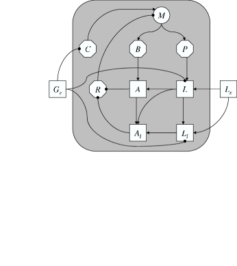
Figure 1. Wiring diagram for the model $H$. Edges in this diagram represent interactions between variables. Arrows indicate positive interactions and circles indicate negative interactions.

2.3.2. Dynamics

The dynamics of $H$ can be computed by evaluating the functions on all possible combinations of vectors $(M,P,B,C,R,A,A_{l},L,L_{l})$ with 0-1 entries (see Section 2.2 for more details). We say that the operon is OFF when the value of the triple $(M,P,B)$ is $(0,0,0)$ and ON when $(M,P,B)=(1,1,1)$. The parameters $L_{e}$ and $G_{e}$ give rise to the following four cases:

1. For $(L_{e},G_{e})=(0,0)$, there is a single steady state, (0,0,0,1,1,0,0,0,0), that corresponds to the operon being OFF.

2. For $(L_{e},G_{e})=(0,1)$, there is a single steady state, (0,0,0,0,1,0,0,0,0), that corresponds to the operon being OFF.

3. For $(L_{e},G_{e})=(1,1)$, there is a single steady state, (0,0,0,0,1,0,0,0,0), that corresponds to the operon being OFF.

4. For $(L_{e},G_{e})=(1,0)$, there is a single steady state, (1,1,1,1,0,1,1,1,1), that corresponds to the operon being ON.

In summary, the model predicts that the lac operon is OFF when extracellular glucose is available or there is neither extracellular glucose or lactose. When extracellular lactose is available and extracellular glucose is not, the model predicts that the operon is ON. That is, the model has two steady states. This is consistent with the reports of bistability as recently as that of [11].

2.3.3. Bistability

We have shown that the model $H$ has essentially two steady states, which correspond to the lac operon being either ON or OFF (one steady state for each set of parameters). These steady states are stable, according to the definition in Appendix C. However, to claim that $H$ exhibits bistability we have to show that for a range of parameters a population of “cells” may exhibit both stable steady states at the same time, corresponding to the lac operon being ON and OFF (see [12] for details); that is, there exists a region of bistability. We will show that if we consider stochasticity in the uptake of the inducer, then bistability can occur. We performed in silico hysteresis experiments similar to the experiments performed by Ozbudak et al. [10].

The experiment to investigate bistability consisted in introducing stochasticity in the uptake of the inducer and vary its value. More precisely, we set the extracellular glucose level to $G_{e}=0$ (the lac operon would be OFF otherwise, independent of the value of the inducer, which we denote by $L_{e}$). Stochasticity in the uptake of the inducer is introduced by using a random variable, $\mathcal{L}_{e}\sim N(\mu,\sigma)$ taken from a normal distribution with mean $\mu$ and variance $\sigma^{2}$. Then we can write $L_{e}$ as a function of $\mathcal{L}_{e}$ defined by

$$L_{e}=\left\{\begin{array}[]{rl}0\text{ if }\mathcal{L}_{e}<1\\ 1\text{ if }\mathcal{L}_{e}\geq 1\end{array}\right.$$

We will refer to this function as the stochastic model.

We start with a population of “cells” with $\mathcal{L}_{e}\sim N(\mu,\sigma)$ and measure whether the operon is induced in those cells after 10 time units; we then decrease the level of the inducer (see Supporting Informationfor details). Similarly, we start with a population of cells with $\mathcal{L}_{e}\sim N(\mu,\sigma)$, measure whether the operon is induced in those cells and increase the level of the inducer. In Figure 2 we started with a population of 100 cells with $\mathcal{L}_{e}\sim N(1.25,0.1)$ and plot the population after 10 time units; we then decrease the level of the inducer to $\mathcal{L}_{e}\sim N(0.75,0.1)$ with a step size of 0.5 (upper panel). We start with a population of 100 cells with $\mathcal{L}_{e}\sim N(0.75,0.1)$ and plot the population after 10 time units; we then increase the level of the inducer to $\mathcal{L}_{e}\sim N(1.25,0.1)$ with a step size of 0.5 (lower panel). We also performed experiments with different values of $\sigma$, $\mu$ and obtained similar results (see Supporting Information).

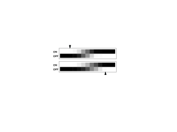
Figure 2. Heat maps of bistability experiments. Grey density determines the percentage of the population that is induced (top row) or uninduced (bottom row) (black:100%, white:0%).

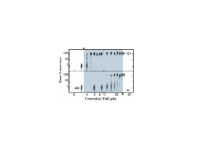
Figure 3. Bistability experiments performed in [10].

We observe in Figure 2 the region of bistability. When we decrease the inducer, an induced-to-uninduced transition can be observed: part of the induced population (top row of upper panel) has turned OFF the lac operon (bottom row of upper panel). On the other hand, when we increase the inducer, an uninduced-to-induced transition can be observed: part of the uninduced population (bottom row of lower panel) has turned ON the lac operon (top row of lower panel). The region where we can see both, cells induced and uninduced, is the region of bistability. We can see that these in silico hysteresis experiments show the same pattern or qualitative behavior as those in [10] (Figure 3). This bistable behavior was not present in model $H$; so it is caused by stochasticity.

3. Reduced Model

An important question is whether the fact that model $H$ has two steady states (either ON or OFF) is caused by the model itself or by topological features and interaction type. We address this question by reducing the model; we reduce the model by deleting vertices but keeping some topological features. If it is the case that topological features and interaction type are the key players for dynamical properties, we would expect the reduced model to have dynamics equivalent to the original model.

3.1. Reducing Boolean networks

We provide a method to reduce a Boolean network and its corresponding wiring diagram. The idea behind the reduction method is the following: the wiring diagram should reflect direct regulation and hence nonfunctional edges should be removed; on the other hand, vertices (variables) can be deleted, without losing important information, by allowing its functionality to be “inherited” to other variables. Step (1) has higher priority than Step (2).

1. Boolean functions are simplified and edges that do not correspond to a Boolean expression are deleted (in the simplification of Boolean functions certain expressions may vanish).

2. Let $a$ be a vertex such that there is no self-loop ($a\circlearrowleft$). Consider all paths of length 2 having $a$ in the middle: $x_{i}\rightarrow a\rightarrow x_{j}$ where $x_{i}$ and $x_{j}$ are vertices. Delete $a$ and replace all edges from/to $a$ by edges from $x_{i}$ to $x_{j}$ (the signs of these edges are given by the sign of the path). Let $f_{a}$ and $f_{x_{j}}$ be the functions for $a$ and $x_{j}$, respectively. Note that $f_{x_{j}}$ is a function of $a$, so we can write it as $f_{x_{j}}(x_{1},\ldots,a,\ldots,x_{n})$. Then the function $f_{x_{j}}$ is replaced by $f_{x_{j}}(x_{1},\ldots,f_{a},\ldots,x_{n})$.

3.2. Reducing the Boolean Network $H$

Let us show some reduction steps applied to the Boolean model of the lac operon.

Figure 4 shows how step 2 is used to delete $R$. We delete $R$ and the edges from/to $R$ are replaced by edges from $A_{l}$ and $A$ to $M$. The sign of these edges are positive because the sign of the corresponding paths are positive.

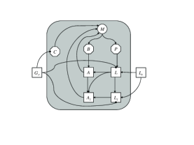
Figure 4. Wiring diagram for the model $H$ before and after using step 2 to delete $R$.

Now let us see how the Boolean functions change when we use step 2. The Boolean functions of model $H$ are given below:

$$\begin{array}[]{ll}H_{M}=\neg R\wedge C&\\ H_{P}=M&H_{B}=M\\ H_{C}=\neg G_{e}&H_{R}=\neg A\wedge\neg A_{l}\\ H_{A}=L\wedge B&H_{A_{l}}=A\vee L\vee L_{l}\\ H_{L}=\neg G_{e}\wedge P\wedge L_{e}&H_{L_{l}}=\neg G_{e}\wedge(L\vee L_{e})\\ \end{array}$$

The Boolean function for $R$ is not needed anymore and the Boolean function for $M$ becomes:

$$\begin{array}[]{ll}H_{M}=\neg(\neg A\wedge\neg A_{l})\wedge C=(A\vee A_{l})\wedge C&H_{P}=M\\ H_{B}=M&H_{C}=\neg G_{e}\\ H_{A}=L\wedge B&H_{A_{l}}=A\vee L\vee L_{l}\\ H_{L}=\neg G_{e}\wedge P\wedge L_{e}&H_{L_{l}}=\neg G_{e}\wedge(L\vee L_{e})\\ \end{array}$$

We can see that the signs of edges are consistent with the Boolean functions.

After deleting $P,B,C,R,A_{l},L_{l}$ we obtain the wiring diagram shown in Figure 5 with Boolean functions given below.

$$\begin{array}[]{ll}H_{M}=\neg G_{e}\wedge(A\vee L\vee L_{e})&\\ H_{A}=L\wedge M&H_{L}=\neg G_{e}\wedge M\wedge L_{e}\\ \end{array}$$

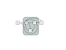
Figure 5. Wiring diagram for the model $H$ after deleting $P,B,C,R,A_{l},L_{l}$.

Now we use step 2 to delete $A$. The new wiring diagram is shown in Figure 6. Notice the self loop at $M$. The Boolean functions are:

$$\begin{array}[]{ll}H_{M}=\neg G_{e}\wedge(L\wedge M\vee L\vee L_{e})&\\ H_{L}=\neg G_{e}\wedge M\wedge L_{e}&\\ \end{array}$$

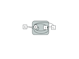
Figure 6. Wiring diagram after deleting $A$.

Using Boolean algebra we have the identity $L\wedge M\vee L=L$; so using step 1 the Boolean functions become:

$$\begin{array}[]{ll}H_{M}=\neg G_{e}\wedge(L\vee L_{e})&\\ H_{L}=\neg G_{e}\wedge M\wedge L_{e}&\\ \end{array}$$

Notice that the self loop at $M$ is actually nonfunctional; then we delete it.

Finally the wiring diagram is given in Figure 7.

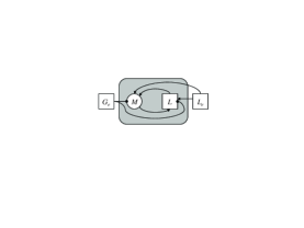
Figure 7. Wiring diagram for the reduced model $h$.

3.3. Reduced model

We reduced the Boolean model $H$ to show that a core subnetwork exists which exhibits bistability. The reduced model, denoted by $h$, contains the variables $M$, $L$, $L_{e}$ and $G_{e}$. The model $h$ is given by

$$\begin{array}[]{ll}h_{M}=\neg G_{e}\wedge(L_{e}\vee L)&\\ h_{L}=\neg G_{e}\wedge L_{e}\wedge M\\ \end{array}$$

where $L_{e}$ and $G_{e}$ are parameters.

3.3.1. Network Topology

The wiring diagram for the model $h$ is shown in Figure 7. We can see that the paths from $G_{e}$ and $L_{e}$ to $M$ are still present in the model; also, the signs of these paths have not changed. Furthermore, the reduction steps have preserved the positive feedback loop involving $M$ and $L$.

Here we have identified the core of the network to be $M$ and $L$. From the reduced model, we can clearly see the roles of the parameters on the core subnetwork.

3.3.2. Dynamics

The state space for the reduced model $h$ is shown in Figure 8. Just as with the model $H$, the reduced model has two different steady states, each corresponding to the operon being ON or OFF. Hence, reduction has preserved the dynamics of the system.

Figure 8. Dynamics of the reduced model $h$ for all parameter values, from left to right: $(L_{e},G_{e})=(0,0),(0,1),(1,1),$ and $(1,0)$.

We observe that the reduced model has only one positive feedback loop, whereas the model $H$ has several more. Since the reduced model still exhibits the ON/OFF switching dynamics, this suggests that this steady-state behavior does not depend on the number of positive feedback loops but simply on the existence of such a loop.

3.3.3. Bistability

Figure 9 shows the results of the bistability experiments performed using model $h$. We can still see the region of bistability for the reduced model. This suggests that bistability does not depend on the number of positive feedback loops but simply on the existence of such a loop and stochasticity. Furthermore, because the feedback loop involves only M and L, this suggests that bistability is maintained by stochasticity and the interaction between the operon (represented by M) and lactose.

Figure 9. Heat maps of bistability experiments for model $h$. The parameters are the same as in Section 2.3.3.

4. Discussion

Many authors have studied the problem of inferring dynamical properties of a system from the network structure [15]. Furthermore, it has been proven for special classes of Boolean networks and ODEs that the network structure contains all the information needed for some dynamical properties [5]. On the other hand, it has been claimed that network topology and sign of interactions are more important than quantitative functionality of the components of a system [2]. To test this hypothesis, we applied the ideas in [2] to lactose metabolism.

The lac operon has been studied extensively and is one of the earliest discovered gene systems that undergoes both positive and negative control. While there are numerous continuous models of the lac operon, few discrete models exist; in fact, that of Setty [14] is the only one known to the authors. The Setty model is a logical (on 4 states) function for the lac genes written in terms of the regulators CRP and LacI that is capable of accurately predicting induction of the operon based on concentration levels of the regulators. Further, this function has been shown to be robust with respect to point mutations [8]. One limitation of this model, however, is that it does not predict bistability, as has been reported and confirmed in [9, 19, 12, 10, 5, 13, 11].

We proposed a Boolean network as a discrete model for the lac operon and included the glucose control mechanisms of catabolite repression and inducer exclusion. We showed that our model exhibits the ON/OFF switching dynamics and that when stochasticity is included, bistability is also observed, in accordance with the work of Santillán and coauthors [19, 12, 13, 11]. Further we presented a reduced model which shows that lac mRNA and lactose form the core of the lac operon, and that this reduced model also exhibits the same dynamics. This suggests that the key to dynamical properties is the topology of the network and signs of interactions. This is consistent with the analysis for the segment polarity network in D. melanogaster made by Albert and Othmer [2].

The use of Boolean networks in modeling has many advantages, such as their mathematical formulation typically being more intuitive for a wider range of scientists than that of differential-equations-based models. Boolean networks are particularly useful in the case where one is interested in qualitatively behavior. For example, our bistability experiments show that bistability can occur when stochasticity is considered and that it depends on topological features rather than the network itself.

A future work may be to extend this model to a multi-state framework, which has the potential to provide a more refined qualitative description of the lac operon. Such a framework may allow for inclusion of other features of the operon, such as multiple promoter and operator regions.

Supporting Information

Appendix A Building Boolean Networks

• Boolean function for $M$: When the concentration of the repressor is high ($R=1$), the production of mRNA will be low ($M=0$) independent of the concentration of CAP ($C$). On the other hand, when the concentration of the repressor is low ($G=0$) and the concentration of CAP is high ($C=1$), mRNA production will be high ($M=1$). In other words, $M$ will be 1 when $R$ is not 1 and $C$ is 1; that is, the future Boolean value of $M$ is NOT $R$ AND $C$. Hence, the Boolean function for $M$ is $H_{M}=\neg R\wedge C$.

• Boolean functions for $P,B$: When mRNA production is high ($M=1$), the production of $P,B$ will be also high ($P=B=1$). Hence, the Boolean functions are $H_{P}=M$ and $H_{B}=M$.

• Boolean function for $C$: When extracellular glucose is abundant ($G_{e}=1$), cAMP synthesis is inhibited ($C=0$). Hence, the Boolean function is $H_{C}=\neg G_{e}$.

• Boolean function for $R$: The concentration of the repressor will be high ($R=1$) only if the concentration of allolactose is not significant, that is, when $A=A_{l}=0$. Hence, the Boolean function is $H_{R}=\neg A\wedge\neg A_{l}$.

• Boolean function for $A$: The concentration of allolactose will be high if the concentrations of permease and extracellular lactose are high. Then, the Boolean function is $H_{A}=L\wedge B$.

• Boolean function for $A_{l}$: The concentration of allolactose will be at least low ($A_{l}=1$) when the concentration of allolactose is high or when the concentration of lactose is high or at least low (it would be converted to allolactose by a basal level of $\beta-galactosidase$). It follows that the Boolean function is $H_{A_{l}}=A\vee L\vee L_{l}$.

• Boolean function for $L$: The concentration of lactose will be high when there is no external glucose, the concentration of permease is high and there is abundant extracellular lactose. Then, the Boolean function is $H_{L}=\neg G_{e}\wedge P\wedge L_{e}$.

• Boolean function for $L_{l}$: When there is no external glucose and the concentration of extracellular lactose is high ($L_{e}=1$), at least a small number of lactose molecules will enter the cell, by diffusion or by a small number of permease molecules (basal level of permease). Also, when there is no external glucose and there is lactose inside the cell ($L=1$), there will be at least a small number of lactose. That is, there will be at least a low concentration of lactose ($L_{l}=1$) when there is not external glucose and the concentration of extracellular or intracellular lactose is high ($L_{e}=1$, $L=1$ respectively). Hence, $H_{L_{l}}=\neg G_{e}(L\vee L_{e})$.

Appendix B Alternative Models

Model $H$ was constructed considering catabolic repression only; two other alternative models may be obtained by considering inducer exclusion only (model $J$) or both, catabolic repression and inducer exclusion (model $K$).

B.1. Network Topology

The Boolean functions for models $J$ and $K$ are given as follows:

Model $J$

$$\begin{array}[]{ll}J_{M}=\neg R\wedge C&\\ J_{P}=M&J_{B}=M\\ J_{C}=1&J_{R}=\neg A\wedge\neg A_{l}\\ J_{A}=L\wedge B&J_{A_{l}}=A\vee L\vee L_{l}\\ J_{L}=\neg G_{e}\wedge P\wedge L_{e}&J_{L_{l}}=\neg G_{e}\wedge(L\vee L_{e})\\ \end{array}$$

Model $K$

$$\begin{array}[]{ll}K_{M}=\neg R\wedge C&\\ K_{P}=M&K_{B}=M\\ K_{C}=\neg G_{e}&K_{R}=\neg A\wedge\neg A_{l}\\ K_{A}=L\wedge B&K_{A_{l}}=A\vee L\vee L_{l}\\ K_{L}=P\wedge L_{e}&K_{L_{l}}=L\vee L_{e}\\ \end{array}$$

The wiring diagrams for models $J$ and $K$ are shown in Figure 10. We can observe that there are paths from $G_{e}$ to $M$ and that they are, for both models, inhibitory. Also, both models have positive feedback loops involving $M$ and no negative feedback loops. We can observe that models $H$, $J$ and $K$ have common topological features.

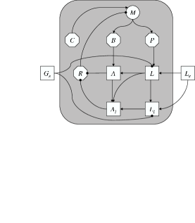
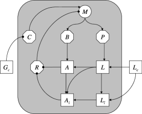
Figure 10. Wiring diagram for the models $J$ and $K$.

B.2. Dynamics

The parameters $L_{e}$ and $G_{e}$ give rise to the following four cases:

Dynamics for model $J$:

1. For $(L_{e},G_{e})=(0,0)$, there is a single steady state, (0,0,0,1,1,0,0,0,0), that corresponds to the operon being OFF.

2. For $(L_{e},G_{e})=(0,1)$, there is a single steady state, (0,0,0,1,1,0,0,0,0), that corresponds to the operon being OFF.

3. For $(L_{e},G_{e})=(1,1)$, there is a single steady state, (0,0,0,1,1,0,0,0,0), that corresponds to the operon being OFF.

4. For $(L_{e},G_{e})=(1,0)$, there is a single steady state, (1,1,1,1,0,1,1,1,1), that corresponds to the operon being ON.

Dynamics for model $K$:

1. For $(L_{e},G_{e})=(0,0)$, there is a single steady state, (0,0,0,1,1,0,0,0,0), that corresponds to the operon being OFF.

2. For $(L_{e},G_{e})=(0,1)$, there is a single steady state, (0,0,0,0,1,0,0,0,0), that corresponds to the operon being OFF.

3. For $(L_{e},G_{e})=(1,1)$, there is a single steady state, (0,0,0,0,0,0,1,0,1), that corresponds to the operon being OFF.

4. For $(L_{e},G_{e})=(1,0)$, there is a single steady state, (1,1,1,1,0,1,1,1,1), that corresponds to the operon being ON.

We can see that models $H$, $J$ and $K$ predict that the lac operon is OFF when extracellular glucose is available or there is neither extracellular glucose or lactose. When extracellular lactose is available and extracellular glucose is not, the model predicts that the operon is ON. That is, all models have two steady states. This shows that qualitative behavior of the model is determined by the topological features of the wiring diagram.

B.3. Reduced Models

Figure 11 shows the wiring diagrams for the models obtained by the reduction of $J$ (model $j$) and reduction of $K$ (model $k$). Their Boolean rules are given by:

reduced model $j$

$$\begin{array}[]{ll}j_{M}=(\neg G_{e}\wedge L_{e})\vee L&\\ j_{L}=L_{e}\wedge M\wedge\neg G_{e}\\ \end{array}$$

reduced model $k$

$$\begin{array}[]{ll}k_{M}=\neg G_{e}\wedge(L_{e}\vee L)&\\ k_{L}=L_{e}\wedge M\\ \end{array}$$

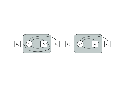
Figure 11. Wiring diagram for the reduced models $j$ and $k$. We can see that in this case they are equal.

We can see that reduced models $j$ and $k$ maintain the main topological features that the reduced model $h$ has, such as the sign of the paths from $L_{e}$ and $G_{e}$ to $M$, and the positive feedback loop involving $M$ and $L$. All reduced models have the same qualitatively behavior; for example, they predict that the operon is OFF for parameters $(L_{e},G_{e})=(0,0),(0,1)$ and $(1,1)$, and ON for $(L_{e},G_{e})=(1,0)$. This provides more evidence that bistability does not depend on the number of positive feedback loops but simply on the existence of such a loop.

Appendix C Bistability

C.1. Stability in a Discrete Framework

Before we explain the details of bistability we need to define the concept of stability in a discrete framework. The definition we use is based on the following idea: a steady state is stable if all nearby trajectories go to it.

C.1.1. Definition of Stability

Let $x$ be a steady state of a Boolean network $S$; that is, $S(x)=x$. We say that $x$ is stable if for any state $y$ such that $|x-y|\leq 1$ then $S^{k}(y)=x$ for some $k$. Where $|x-y|$ is the Hamming distance that gives the number of nonzero values of $x-y$; that is, the number of components in which $x$ and $y$ differ.

C.1.2. The two steady states of the lac operon operon are stable

For any set of parameters there is only one steady state, the lac operon is either ON or OFF. Hence, the definition of stable is clearly satisfied; the ON and OFF states are stable.

C.2. Stochastic Model

Stochasticity in the uptake of the inducer is introduced by using a random variable, $\mathcal{L}_{e}\sim N(\mu,\sigma)$ (normal distribution with mean $\mu$ and variance $\sigma^{2}$); $L_{e}$ is then a function of $\mathcal{L}_{e}$ defined by $L_{e}=0$ if $\mathcal{L}_{e}<1$ and $L_{e}=1$ if $\mathcal{L}_{e}\geq 1$. We will refer to this function as the stochastic model, $S$.

More precisely, the stochastic model is given by:

$$\begin{array}[]{ll}S_{M}=\neg R\wedge C&S_{P}=M\\ S_{B}=M&S_{C}=\neg G_{e}\\ S_{R}=\neg A\wedge\neg A_{l}&S_{A}=L\wedge B\\ S_{A_{l}}=A\vee L\vee L_{l}&S_{L}=\neg G_{e}(P\wedge L_{e})\\ S_{L_{l}}=\neg G_{e}(L\vee L_{e})&S_{L_{e}}=\delta(\mathcal{L}_{e})=\delta(N(\mu,\sigma))\\ \end{array}$$

Where the function $y=\delta(x)$ is defined by $y=0$ if $x<1$ and $y=1$ if $x\geq 1$. $G_{e}\in\{0,1\}$ and $\mathcal{L}_{e}\sim N(\mu,\sigma)$ (actually $\mu$ and $\sigma$) are parameters for the stochastic model. On the other hand, when we say that we decrease (increase) the value of the inducer me refer to decreasing (increasing) the value of $\mu$ and use the model with this new value.

For example, for $G_{e}=0$, $\mu=1.1$ and $\sigma=.1$ the model is

$$\begin{array}[]{ll}S_{M}=\neg R\wedge C&S_{P}=M\\ S_{B}=M&S_{C}=\neg 0\\ S_{R}=\neg A\wedge\neg A_{l}&S_{A}=L\wedge B\\ S_{A_{l}}=A\vee L\vee L_{l}&S_{L}=P\wedge L_{e}\\ S_{L_{l}}=L\vee L_{e}&S_{L_{e}}=\delta(N(1.1,.1))\\ \end{array}$$

As an example let us generate a time series during 3 time units. Let the current state be $s_{0}=(0,1,1,0,1,0,1,0,0,0)$, the next state, $s_{1}$, is given by:

$$\begin{array}[]{ll}S_{M}=\neg 1\wedge 0=0&S_{P}=0\\ S_{B}=0&S_{C}=1\\ S_{R}=\neg 0\wedge\neg 1=0&S_{A}=0\wedge 1=0\\ S_{A_{l}}=0\vee 0\vee 0=0&S_{L}=1\wedge 0=0\\ S_{L_{l}}=0\vee 0=0&S_{L_{e}}=\delta(N(1.1,.1))=\delta(1.1236)=1\\ \end{array}$$

that is, $s_{1}=(0,0,0,1,0,0,0,0,0,1)$. The next state, $s_{2}$, is given by:

$$\begin{array}[]{ll}S_{M}=\neg 0\wedge 1=1&S_{P}=0\\ S_{B}=0&S_{C}=\neg 0=1\\ S_{R}=\neg 0\wedge\neg 0=1&S_{A}=0\wedge 0=0\\ S_{A_{l}}=0\vee 0\vee 0=0&S_{L}=0\wedge 1=0\\ S_{L_{l}}=0\vee 1=1&S_{L_{e}}=\delta(N(1.1,.1))=\delta(0.9998)=0\\ \end{array}$$

that is, $s_{2}=(1,0,0,1,1,0,0,0,1,0)$. If we now increase the value of the inducer to $\mathcal{L}_{e}\sim N(1.2,.1)$, the next state, $s_{3}$ is given by:

$$\begin{array}[]{ll}S_{M}=\neg 1\wedge 1=0&S_{P}=1\\ S_{B}=1&S_{C}=\neg 0=1\\ S_{R}=\neg 0\wedge\neg 0=1&S_{A}=0\wedge 0=0\\ S_{A_{l}}=0\vee 0\vee 1=1&S_{L}=0\wedge 0=0\\ S_{L_{l}}=0\vee 0=0&S_{L_{e}}=\delta(N(1.2,.1))=\delta(1.1529)=1\\ \end{array}$$

that is, $s_{3}=(0,1,1,1,1,0,1,0,0,1)$.

C.3. Heat Maps

In Figure 2 we started with a population of 100 cells with $\mathcal{L}_{e}\sim N(1.25,.1)$ and plot the population after 10 time units; we then decrease the level of the inducer to $\mathcal{L}_{e}\sim N(0.75,.1)$ with a step size of .5 (upper panel). We start with a population of 100 cells with $\mathcal{L}_{e}\sim N(0.75,.1)$ and plot the population after 10 time units; we then increase the level of the inducer to $\mathcal{L}_{e}\sim N(1.25,.1)$ with a step size of .5 (lower panel). This figure shows that we can have both stable steady states at the same time; that is, some cells are induced and other uninduced. This bistability behavior was not present with model $H$; hence it was caused by the stochasticity in the uptake of the inducer. Figure 12 shows the same experiment with $\sigma=.15$, $\sigma=.2$, $\sigma=.05$ and $\sigma=.03$. We can still observe the induced-to-uninduced (upper panel) and uninduced-to-induced transitions. We also performed experiments using models $J$ and $K$ and obtained similar results. The bistable behavior of the models seem to be caused by the topological features of the models such as the sign of the paths from $L_{e}$ and $G_{e}$ to $M$ and the existence of the feedback loop involving $M$.

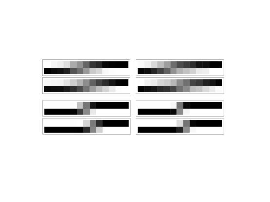
Figure 12. Heat maps of bistability experiments using $\sigma=.15,.2$ (top) and $\sigma=.05,.03$ (bottom).

Figure 13 shows the heat maps for models $J$ and $K$. We can see that both models exhibit bistability.

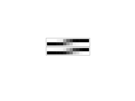
Figure 13. Heat maps of bistability experiments for models $J$ and $K$. The parameters are the same as for $H$.

References

- [1] B. Aguda and A. Goryachev. From pathways databases to network models of switching behavior. PLoS Computational Biology, 3(9):1674–1678, 2007.
- [2] R. Albert and H. Othmer. The topology of the regulatory interactions predicts the expression pattern of the segment polarity genes in Drosophila melanogaster. Journal of Theoretical Biology, 223:1–18, 2003.
- [3] B. Goodwin. Temporal Organization in Cells. Academic Press, New York, 1963.
- [4] A. Griffiths, J. Miller, D. Suzuki, R. Lewontin, and W. Gelbart. Introduction to Genetic Analysis. W. H. Freeman and Co., New York, 1999.
- [5] Á. Halász, V. Kumar, M. Imieliński, C. Belta, O. Sokolsky, S. Pathak, and H. Rubin. Analysis of lactose metabolism in E.coli using reachability analysis of hybrid systems. IET Systems Biology, 1(2):130–148, 2007.
- [6] F. Jacob and J. Monod. Genetic regulatory mechanisms in the synthesis of proteins. Journal of Molecular Biology, 3:318–356, 1961.
- [7] A. Jarrah, R. Laubenbacher, and H. Vastani. DVD: Discrete visualizer of dynamics. Available at http://dvd.vbi.vt.edu.
- [8] A. Mayo, Y. Setty, S. Shavit, A. Zaslaver, and U. Alon. Plasticity of the cis-regulatory input function of a gene. PLoS Biology, 4(4):0555–0561, 2006.
- [9] A. Novick and M. Weiner. Enzyme induction as an all-or-none phenomenon. Proceedings of the National Academy of Sciences of the United States of America, 43(7):553–566, 1957.
- [10] E. Ozbudak, M. Thattai, H. Lim, B. Shraiman, and A. van Oudenaarden. Multistability in the lactose utilization network of Escherichia coli. Nature, 427:737–740, 2004.
- [11] M. Santillán. Bistable behavior in a model of the lac operon in Escherichia coli with variable growth rate. Biophysical Journal, 94(6):2065 2081, 2008.
- [12] M. Santillán and M. Mackey. Influence of catabolite repression and inducer exclusion on the bistable behavior of the lac operon. Biophysical Journal, 86(3):1282–1292, 2004.
- [13] M. Santillán, M. Mackey, and E. Zeron. Origin of bistability in the lac operon. Biophysical Journal, 92(11):3830–3842, 2007.
- [14] Y. Setty, A. Mayo, M. Surette, and U. Alon. Detailed map of a cis-regulatory input function. Proceedings of the National Academy of Sciences of the United States of America, 100(13):7702 7707, 2003.
- [15] E. Sontag, A. Veliz-Cuba, R. Laubenbacher, and A. Jarrah. The effect of negative feedback loops on the dynamics of boolean networks. Biophysical Journal, 95:518–526, 2008.
- [16] M. van Hoek and P. Hogeweg. In silico evolved lac operons exhibit bistability for artificial inducers, but not for lactose. Biophysical Journal, 91(8):2833 2843, 2006.
- [17] M. van Hoek and P. Hogeweg. The effect of stochasticity on the Lac operon: An evolutionary perspective. PLoS Computational Biology, 3(6):1071–1082, 2007.
- [18] P. Wong, S. Gladney, and J. Keasling. Mathematical model of the lac operon: Inducer exclusion, catabolite repression, and diauxic growth on glucose and lactose. Biotechnology Progress, 13(2):132–143, 1997.
- [19] N. Yildirim, M. Santillán, D. Horike, and M. Mackey. Dynamics and bistability in a reduced model of the lac operon. Chaos, 14(2):279–292, 2004.