Evidence for an intermediate line region in AGN’s inner torus region and its evolution from narrow to broad line Seyfert I galaxies

Abstract

A two-components model for Broad Line Region (BLR) of Active Galactic Nuclei (AGN) has been suggested for many years but not widely accepted (e.g., Hu et al. 2008; Sulentic et al. 2000; Brotherton et al. 1996; Mason et al. 1996). This model indicates that the broad line can be described with superposition of two Gaussian components (Very Broad Gaussian Component (VBGC) and InterMediate Gaussian Component (IMGC)) which are from two physically distinct regions; i.e., Very Broad Line Region (VBLR) and InterMediate Line Region (IMLR). We select a SDSS sample to further confirm this model and give detailed analysis to the geometry, density and evolution of these two regions. Micro-lensing result of BLR in J1131-1231 and some unexplained phenomena in Reverberation Mapping (RM) experiment provide supportive evidence for this model. Our results indicate that the radius obtained from the emission line RM normally corresponds to the radius of the VBLR, and the existence of the IMGC may affect the measurement of the black hole masses in AGNs. The deviation of NLS1s from the M-sigma relation and the Type II AGN fraction as a function of luminosity can be explained in this model in a coherent way. The evolution of the two emission regions may be related to the evolutionary stages of the broad line regions of AGNs from NLS1s to BLS1s. Based on the results presented here, a unified picture of hierarchical evolution of black hole, dust torus and galaxy is proposed.

1 Introduction

Type I AGNs are often classified into two subclasses according to the Full Width at Half Maximum (FWHM) of their broad H$\beta$ lines. Those AGNs with FWHM greater than approximately 2000 km$\cdot$s^-1 are called Broad Line Seyfert 1 (BLS1), and those with FWHM less than approximately 2000 km$\cdot$s^-1 are called Narrow Line Seyfert 1 (NLS1). There is a tight correlation between the black hole mass and the stellar velocity dispersion of the bulge of normal galaxies, the so called M-sigma relation (e.g. Magorrian et al. 1998; Gebhardt, et al. 2000; Tremaine et al. 2002; Marconi & Hunt 2003; Ferrarese & Ford 2005). BLS1s are found also to follow this relation well (Greene & Ho 2006). However, NLS1s seem to deviate from this relation; they seem to have much smaller masses or much higher stellar velocity dispersions (e.g., Wang & Lu 2001; Bian & Zhao 2004; Zhou et al. 2006; Komossa & Xu 2007). We call this under-massive black hole problem of NLS1s. Since there are a lot of uncertainties on measuring the black hole mass and sigma (Decarli et al. 2008; Komossa & Xu 2007; Komossa 2008; Komossa et al. 2008), it is difficult to determine whether the deviation reflects an intrinsic mass or/and sigma difference between the NLS1s and BLS1s, or it is only caused by the measurements. NLS1s also show softer X-ray spectra, strong Fe II emission, rapid continuum variation, and high accretion rate; the last one may partly be caused by the incorrect measurement of the black hole mass (e.g., Grupe & Mathur 2004; Komossa 2008). However, Williams et al. (2004) found some optically defined NLS1s are different from those defined by X-ray selected NLS1s, suggesting that strong, ultrasoft X-ray emission is not a universal characteristic of NLS1s and challenging the current paradigm that NLS1s accrete near the Eddington limit.

In the simple unified model for AGN, Type I and Type II objects differ only in terms of the angle between the observer’s line of sight and the normal axis of a dusty torus (Urry & Padovani 1995). SEDs of QSOs also imply that the location of the inner wall of torus is determined by the sublimation of dust by the central radiation (e.g. Kobayashi et al. 1993; Elvis et al. 1994). It is widely accepted that $R_{\rm{torus}}\propto L^{0.5}$ (e.g., Elitzur 2006; Peterson 2007; Nenkova 2008a), consistent with that predicted by the toy model of Krolik & Begelman (1988). Reverberation mapping (RM) based on infrared emission also supports this relation (Suganuma et al. 2006).

Many observations show that the fraction of type I AGNs increases with luminosity (Ueda et al. 2003; Hasinger 2004, 2005; Steffen et al. 2003, 2004; Barger et al. 2005; Wang et al. 2005), i.e., brighter AGNs are mostly type I AGNs. This is also equivalent observationally to the situation that it is less probable to find very luminous type II AGNs (mostly Seyfert II galaxies) in a random sample of AGNs. We call this under-populated luminous type II problem of Seyfert galaxies. However, the standard receding torus model with constant height first suggested by Lawrence (1991) failed to describe this luminosity fraction, and thus a modified receding torus whose height slightly increases with luminosity with the relation $h\propto L^{0.23}$ is needed (Simpson 2005). Based on the luminosity fraction for Type I AGN, Wang et al. (2005) obtained a relation between covering factor of the torus and luminosity, $\log{C}=-0.17\log{L_{x}}-0.36$. The variation of covering factor with luminosity may be totally caused by the receding of the inner torus (Wang et al. 2005).

Clearly both the broad line regions and the dust tori of AGNs show strong dependence of luminosity, yet the physical connections between these two key ingredients of AGN’s unification scheme are not yet fully understood. It is also not clear if the luminosity dependence of dust torus and broad line region is simultaneously related to both problems of under-massive black holes in NLS1 galaxies and under-populated luminous type II Seyfert galaxies. Progress towards solving these problems may shed new lights to the understanding the hierarchical evolution of AGN and its host galaxy, as well as the feeding, fueling and growth of supermassive black holes. In this paper we attempt to address both problems in a coherent way by studying a sample of SDSS AGNs with strong broad emission lines.

The geometry and kinematics of broad line region in AGN have been studied for about three decades but far from been fully understood. There are mainly two kinds of views to interpret the structure of BLR based on the profiles of balmer lines. One interprets the profile as a Gaussian/Lorentz profile and BLR as a extended region has different projected velocity distributions (e.g., Goncalves et al. 1999; Collin et al. 2006). The other model is that the profile is a superposition of double Gaussian profiles (Intermediate Component+Very Broad Component in Hu et al. 2008; Broad Component+Very Broad Component in Sulentic et al, 2000 and Marziani et al. 2009. These two components will be re-named as InterMediate Gaussian Component (IMGC)+Very Broad Gaussian Component(VBGC) in this paper.), which come from two physically distinct emission regions due to their substantial differences in the line widths (e.g., Hu et al. 2008; Sulentic et al. 2000; Brotherton et al. 1996; Mason et al. 1996); we call these two regions Very Broad Line Region (VBLR) and InterMediate Line Region (IMLR). For the two-components model, the results from these papers are not consistent with each other and the physical interpretations to these two emission regions are also different. Sulentic et al (2000) suggested that VBGC is likely to arise in an optically thin region close to the central source which is slightly red-shifted, whereas Hu et al. (2008) concluded that IMGC is systematically red-shifted and may come from the inflow. In addition, the study of partially obscured quasars suggests that there is an inner narrow line region covered by dust which may be consistent with our IMLR (Zhang et al. 2009). The existence of these two emission regions need to be confirmed further and their dynamical and physical properties also need to be further studied. For this purpose, we select a SDSS sample with strong H$\alpha$, H$\beta$ and H$\gamma$ lines, and decompose these balmer lines based on the two-components model. Our goal is to provide further evidence for this model, carry out more detailed analysis about the dynamics and evolution of these two emission regions, and ultimately to understand the above two problems (The under-massive black hole problem of NLS1s and The under-populated luminous type II problem of AGNs) in a coherent way.

This paper is organized in the following way. Detailed decomposition and FWHM measurement are described in Section 2. In Section 3 we present H$\alpha$, H$\beta$, and H$\gamma$ decomposition and statistical analysis. In section 4 we confirm the two-components model based on the line decomposition and give detailed analysis of these two emission regions. Section 5 presents other supporting evidence for this model. Section 6 shows that this model provides a coherent interpretation to the two problems. Section 7 is conclusion and discussion. The continuum luminosity and some other parameters of AGNs are directly taken from Table 2 in La Mura et al. (2007). FWHM is defined as FWHM of the whole line, FWHMi means FWHM of the IMGC and FWHMb represents FWHM of the VBGC when they are not clear in the context. The unit is km s^-1 for the “width” of all lines and components, as well as the inferred velocity, throughout this manuscript.

2 Line decomposition and FWHM measurement

The sample contains 90 objects with clear H$\alpha$, H$\beta$, and H$\gamma$ line profiles that can be decomposed. They are selected by La Mura et al. (2007) from SDSS 3 based on their balmer line intensities. Narrow emission lines have already been removed by La Mura et al. (2007) from the spectra we adopted, with templates extracted from OIII and with compatible width; the detailed description on how they have produced the broad line spectral catalog we used here is presented in La Mura et al. (2007). Therefore all analysis and discussions in this paper do not concern with those narrow lines. 21 of them are classified as NLS1s. A two-component model (a disk line plus a Gaussian component) to fit the profile of the broad lines has been presented by Popović et al. (2008) and Bon et al. (2006). We first tried this model. However, the fitting is not acceptable statistically for most of the objects in this sample. Instead, a double Gaussian component model can fit the profile very well.

First, we fit H$\alpha$ and H$\beta$ lines freely with two Gaussian components, i.e., a VBGC and an IMGC; a wavelength deviation of 10 $\AA$ from their rest frame wavelength is allowed in the fitting for the central value of the two components. When the IMGC is statistically insignificant, we refit the spectrum with just one Gaussian component. Our results are generally consistent with the results reported by Mullaney & Ward (2008); they decomposed nine H$\alpha$ lines, three of which only need one Gaussian component. The decomposition of H$\alpha$ is thus quite straight forward. However, it is more complicated to decompose the H$\beta$ lines, because of the contamination of a broad line He I at 4922 $\AA$ and Fe II on the red wing of H$\beta$ (Véron et al. 2002; Mullaney & Ward 2008). We thus add a Gaussian component with centers ranging from 4922 $\AA$ to 4940 $\AA$ when necessary. The profile of the FeII is not important here. Due to the above complication and the relative weakness of the H$\beta$ lines, sometimes there are relatively large uncertainties in the H$\beta$ line decomposition.

Second, with the result of the first step, to every H$\alpha$ and H$\beta$ line, we get the width of their VBGCs, $V_{\rm{H}\alpha}$ and $V_{\rm{H}\beta}$, respectively. If $V_{\rm{H}\alpha}>V_{\rm{H}\beta}$, we refit the H$\alpha$ by requiring $|V_{\rm{H}\alpha}-V_{\rm{H}\beta}|\leq 0.1V_{\rm{H}\beta}$ and fit the corresponding H$\gamma$ by also requiring $|V_{\rm{H}\gamma}-V_{\rm{H}\beta}|\leq 0.1V_{\rm{H}\beta}$. Conversely, if $V_{\rm{H}\alpha}<V_{\rm{H}\beta}$, we refit the H$\beta$ by requiring $|V_{\rm{H}\alpha}-V_{\rm{H}\beta}|\leq 0.1V_{\rm{H}\alpha}$ and fit the corresponding H$\gamma$ by also requiring $|V_{\rm{H}\gamma}-V_{\rm{H}\alpha}|\leq 0.1V_{\rm{H}\alpha}$. The motivation of the above requirement is to ensure the fittings are physical, i.e., the VBGCs of these three lines are produced from regions with radius not very different, since $dR=-2VdV$, if the same gravitationally-bound gas dynamics applies to all three lines. We do not impose the same radius for the emission line regions for the three VBGCs, because RM measurements have found different delay times for different emission lines (e.g., Peterson & Wandel 1999; Kaspi et al. 2000). The difficulty of fitting H$\gamma$ comes from its weak flux, roughly about two times weaker than H$\beta$. Since H$\alpha$ has a clear red wing, it also helps to reduce the influence of Fe II contamination in H$\beta$ fitting.

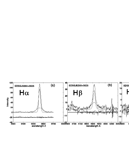
Figure 4: Decompositions of H$\alpha$, H$\beta$, H$\gamma$ of SDSSJ0250+0025. Its H$\beta$ and H$\alpha$ lines behave similarly as SDSSJ1344+4416 shown in Fig.1(a1) and Fig.1(a2), respectively. The H$\gamma$ line lost its VBGC, which can be caused by confusion in the continuum subtraction, when it is very weak and broad.

A single Gaussian component model is not acceptable for the majority of the sources in this sample. This is consistent with the results of Collin et al. (2006), who found that most broad line profiles of AGNs are non-Gaussian and deviations from a Gaussian profile are correlated with the properties of AGNs. Almost all of the spectra (88/90 for H$\alpha$ and H$\beta$, 74/90 for H$\gamma$) can be fitted very well with this double Gaussian components model. For this reason, model lines based on two Gaussian components are used to measure the FWHM of the whole line (e.g., Greene & Ho 2005). Since the error estimate is very complex, we just use the typical error of 10% of FWHM, following Greene & Ho (2005) and Vestergaard & Peterson (2006). Those that do not fit well have been excluded from our analysis. Several typical decomposition examples are presented in Fig.1 and Fig.4. The decomposition parameters of these objects are presented in the table.

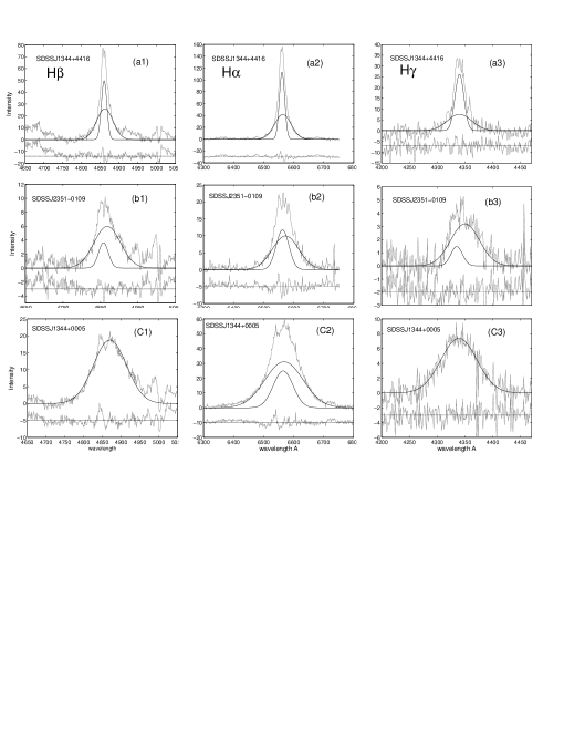
Figure 1: Decomposition examples of broad H$\beta$, H$\alpha$ and H$\gamma$ lines. From (a) to (c), FWHM of the line increases, and the IMGC becomes weaker and may disappear sometimes, e.g., in subpanels c1 & c3. Note that for in subpanel c2, the IMGC of H$\alpha$ line is still detectable, in contrast to H$\beta$ and H$\gamma$ lines, because the IMGC of H$\alpha$ is normally much stronger than H$\beta$ and H$\gamma$ lines (see Fig.8 for line intensity ratios between these three lines).)

Since these parameters are somewhat degenerated in the fitting, Monte Carlo simulations are carried out to examine if this degeneration affects the reliability of our spectral decompositions. As shown in Fig.2, 80 simulated spectra are produced, with each one composed of an IMGC and a VBGC; each parameter of these Gaussian components is a random choice from a corresponding parameter group which covers the similar parameter range in our sample. Proper noise is also added to each simulated spectrum. We then decompose these simulated spectra and obtain the fitted parameters. Fig.2 shows that the fitted parameters do not deviate from the initially set parameters significantly.

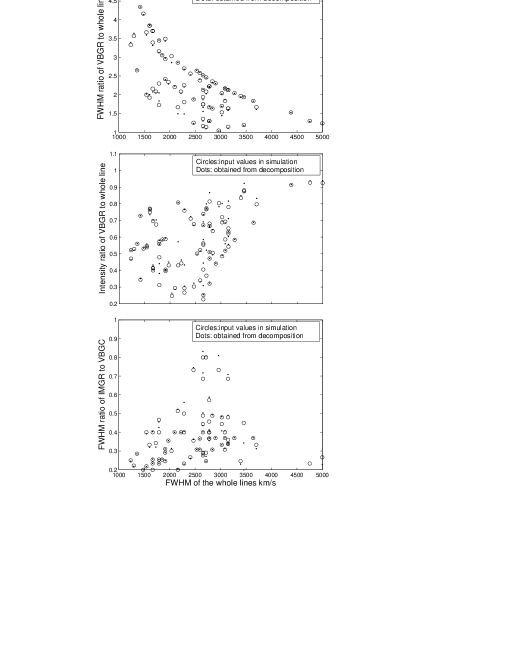
Figure 2: Monte Carlo simulations of spectral decomposition. It can be seen that the decomposed spectral parameters agree with input values quite well, indicating that degenerations in spectral decompositions are not serious.

3 Analysis of H$\beta$, H$\alpha$ and H$\gamma$ lines

3.1 H$\beta$ lines

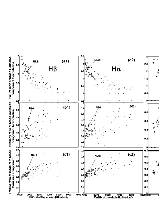
Figure 3: Statistical analysis of broad H$\beta$, H$\alpha$ and H$\gamma$ lines. With the FWHM increasing, FWHM ratio of VBGC to the whole line becomes smaller and finally reaches unity, the intensity ratio of the VBGC to the whole line becomes larger and finally also reaches unity, and the IMGC becomes broader and weaker. The uncertainty is roughly as large as the dispersion.

First, we focus on H$\beta$ lines; several examples are shown in Fig.1 (a1, b1 & c1) and Fig.4 (b). The statistical analysis is presented in Fig.3 (a1, b1 & c1). The VBGC has a much larger FWHM than the whole line when FWHM of the whole line is small. The FWHM ratios range from 1.5 to 4 in the NLS1 group which lie on the left of Fig.3(a1). The intensity ratio of the VBGC to the whole line is about 0.6 in these objects. This means that for NLS1s the IMGC has an intensity comparable to the VBGC, and consequently the FWHM of the whole line of NLS1s is dominated by the IMGC. With FWHM increasing, the IMGC becomes weaker and finally disappeared, which can be seen from Fig.3(b1), in which the intensity ratio of the VBGC to the whole line reaches unity when FWHM of the whole line reaches about 5000 km$\cdot$s^-1. Naturally, the FWHM ratio of the VBGC to the whole line also reaches unity. The whole line can thus be simply described by a single VBGC and the VBGC becomes totally dominant. This trend agrees with that obtained by Hu et al. (2008), who have shown that most of the AGNs with very large black hole masses (normally with largest FWHM) do not need two components for their broad H$\beta$ lines. Our result also agrees with Collin et al. (2006), who found that NLS1s seem to have a prominent narrower component (the IMGC identified in our work) on top of a broad Gaussian profile (the VBGC identified in our work).

In Fig.3(c1), FWHM ratio of the IMGC to the VBGC becomes larger with increasing FWHM. It ranges from $0.2$ to $0.6$, which is another reason for the FWHM of the whole line reaching the FWHM of the VBGC. It indicates that the IMGC also becomes broader when it becomes weaker. The points lie on $y=0$ of the bottom picture represent the objects which have only a single Gaussian component. The three points with maximum FWHM (but still with two Gaussian components) fall off the trend slightly, due to perhaps the large uncertainties in fitting when the intensity of the IMGC becomes very low.

Compared to Fig.2, the correlations in Fig.3 are much tighter, suggesting that the two-components decomposition is physically meaningful, not just a mathematical convenience. Moreover, the systematical evolution show in Fig.3 suggests that the two components are physically distinct, and both components responses to a common source.

3.2 H$\alpha$ lines

Fig.1 (a2, b2 & c2) and Fig.4 (a) are several decomposition examples for H$\alpha$ lines. They behave similarly when FWHM is small. However when FWHM is large, the IMGC is very broad and strong. Statistical analysis is shown in Fig.3 (a2, b2 & c2) in a similar manner to H$\beta$ lines. The obvious difference is that the number of points near unity in panel (b2) is less than that in panel (b1) for H$\beta$ lines; only a weakly increasing trend can be seen in panel (b2). This means that the IMGC is still strong even when FWHM reaches about 5000 km$\cdot$s^-1.

3.3 H$\gamma$ lines

H$\gamma$ lines behave similarly to H$\beta$ lines as shown Fig.1 (a3, b3 & c3) and Fig.4 (c); when FWHM is very large, only a single Gaussian component (the VBGC) is required to fit the profile. However, when FWHM is very small, a large number of H$\gamma$ lines loose the VBGC, i.e, only the IMGC is required to fit the line, because most of their FWHM are very close to the IMGCs of their H$\beta$ lines. The points lie on the x-axis in Fig.3 (b3) are the cases when the H$\gamma$ lines are described by a single IMGC; an example is presented in Fig.4 (c). However some of the single Gaussian component H$\gamma$ lines have FWHM neither close to the VBGC nor close to the IMGC of the corresponding H$\beta$ lines, therefore we exclude these points in our analysis. The loss of the VBGCs may be caused by the weak intensity of H$\gamma$, since its VBGC is particularly weak when FWHM is small, which can cause confusion in the continuum subtraction. The gap pointed by an arrow in Fig.3 (b3) also reveals a sudden decrease of the intensity of the broad Gaussian component when it is very weak.

3.4 FWHM evolution with luminosity

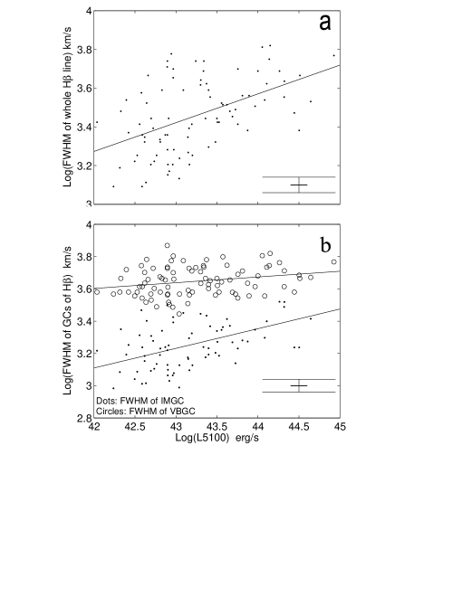
Figure 5: Upper panel shows that FWHM of the whole H$\beta$ line increase with luminosity of the source. Lower panel is the correlation between FWHM of a single Gaussian component (VBGC/IMGC) and luminosity. The sum squared error (SSE) of the L5100-FWHM fitting in (a) is 2.34 (88 points), SSE of the L5100-FWHMb fitting in (b) is 0.66 (88 points) and SSE of the L5100-FWHMi fitting is 1.07 (74 points). The correlation of a single Gaussian component’ FWHM and luminosity is tighter than that of the whole line. The typical uncertainty is plotted in the corner

Previous works suggested that a highly significant correlation exists between FWHM(H$\beta$) and source luminosity (e.g., Joly et al. 1985; Corbett et al. 2003). More recent work with a larger sample which spans a FWHM range from 1000 to 16000 km s^-1 showed that the correlation is not so strong but still statistically significant; the correlation in this large sample is likely driven by the minimum FWHM trend (Marziani et al 2009). Fig.5a presents this correlation in our sample; the correlation is more obvious in this smaller sample than in Marziani et al (2009), and it is very similar to the correlation in Joly et al (1985). The extremely broad H$\beta$ (FWHM $>$ about 7000 km s^-1) may have a rather different line profile and may originate from a different physical region from the less broad H$\beta$ (e.g., Strateva et al. 2003; Eracleous et al. 2003), therefore the analysis with only mediate broad (FWHM $<$ about 7000 km s^-1) H$\beta$ with the same line profile seems to be more meaningful. Fig.5b shows that the logarithm of FWHM of the VBGC or IMGC increases with the logarithm of luminosity in a more linear way than FWHM of the whole line. This may indicate that FWHM of VBGC or IMGC is more physical than FWHM of the whole line. On the other hand, Fig.5b also shows that FWHM of IMGC increases with luminosity much faster than VBGC; the two components has a trend to merge into one. This trend will be confirmed in another way in section 4.1. Therefore FWHM evolution also supports the picture that the broad line region is composed of two physically distinct regions.

4 Dynamics and physical properties of the two emission regions

4.1 Evolution of the two emission regions

We assume that the two Gaussian components come from two distinct regions, and both of the these two regions (VBLR and IMLR) are bounded by the central black hole’s gravity. We therefore have

$$f_{1}^{2}\frac{V_{\rm{VBLR}}^{2}}{R_{\rm{VBLR}}}=\frac{GM_{\rm{BH}}}{R_{\rm{VBLR}}^{2}},$$ (1)

and

$$f_{2}^{2}\frac{V_{\rm{IMLR}}^{2}}{R_{\rm{IMLR}}}=\frac{GM_{\rm{BH}}}{R_{\rm{IMLR}}^{2}}.$$ (2)

Equation (1) and (2) lead to

$$R_{\rm{IMLR}}=(\frac{f_{1}V_{\rm{VBLR}}}{f_{2}V_{\rm{IMLR}}})^{2}R_{\rm{VBLR}}=C_{0}(\frac{V_{\rm{VBLR}}}{V_{\rm{IMLR}}})^{2}R_{\rm{VBLR}},\\$$ (3)

where

$$C_{0}=(\frac{f_{1}}{f_{2}})^{2}.\\$$ (4)

We assume that $C_{0}$ is a constant for all sources, because currently we cannot determine the exact geometry and velocity distribution of gases in the IMLR. The validity of this assumption and the exact value of $C_{0}$ needs to be determined with further studies of more observation data. For convenience we simply redefine $R_{\rm{IMLR}}=R_{\rm{IMLR}}/C_{0}$ for the rest of this paper, i.e., we only consider the special case when $C_{0}=1$ (see section 5.2 for a tentative support to this rather arbitrary choice).

RM is used to measure radius of the BLR, which is related to an AGN’s continuum luminosity by the following empirical Radius-Luminosity relation (Kaspi et al. 2005):

$$\log{\frac{R_{\rm{BLR}}}{\rm{lt-days}}}=(0.69\pm 0.05)\log{\frac{\lambda L_{\lambda}(5100\AA)}{\rm{erg}\cdot\rm{s}^{-1}}}-29.0\pm 2.2,$$ (5)

or the starlight-corrected R-L relation (Bentz et al. 2006):

$$\log{\frac{R_{\rm{BLR}}}{\rm{lt-days}}}=(0.518\pm 0.039)\log{\frac{\lambda L_{\lambda}(5100\AA)}{\rm{erg}\cdot\rm{s}^{-1}}}-21.2\pm 1.7.$$ (6)

We use equation (6) to calculate $R_{\rm{BLR}}$ throughout this work, unless indicated otherwise. Equation (5) is only used in Section 4.4 where a comparison is made.

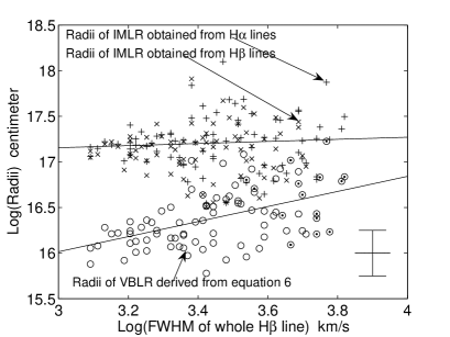
Figure 6: Correlation of the radii of IMLR and VBLR with the FWHM of the whole H$\beta$ line. Radii are plotted in logarithm scale. Circles are the VBLR radius, “$\times$” represent IMLR radii derived from H$\beta$ lines and “$+$” are obtained from H$\alpha$ lines. Circles filled with dots represent the objects missing the IMGC. Least-absolute-residuals fitting results are also plotted: for IMLR $\log{R}=0.115(\pm 0.3)\log{\rm{FWHM}}+16.81(\pm 1.1)$, and for VBLR $\log{R}=0.8253(\pm 0.27)\log{\rm{FWHM}}+13.54(\pm 1)$. It is interesting to note that the radius of IMLR is not correlated with the FWHM of the whole H$\beta$ line. The typical uncertainty is plotted in the corner.

Because RM is used to measure radius of BLR, one might expect that it would normally measure the radius of the innermost emission-line region, i.e., the VBLR in our model (see discussion on this issue in section 5.2). Therefore, the radius calculated from $R_{\rm{BLR}}\sim$L5100 relation is taken as $R_{\rm{VBLR}}$. Consequently, we can calculate the radius of IMLR from equation (3). Both H$\alpha$ and H$\beta$ lines can be used to do this calculation. Because they seem to behave slightly differently in the line evolution, $R_{\rm{IMLR}}$ is obtained from H$\alpha$ and H$\beta$ lines separately. Fig.6 is the evolution of $R_{\rm{VBLR}}$ and $R_{\rm{IMLR}}$ with FWHM. IMLR radii derived from H$\alpha$ and H$\beta$ lines have only subtle differences. The IMLR radius just varies around a constant with increasing FWHM, i.e. does not have a systematic increase or decrease. On the other hand, VBLR radius becomes larger with increasing FWHM. VBLR and IMLR are clearly separated with FWHM$<2500$ km$\cdot$s^-1 as we can see in Fig.6. The circles filled with dots represent the objects whose lines are fitted well with a single (very) broad Gaussian component; they appear in the Fig.6 with largest FWHM.

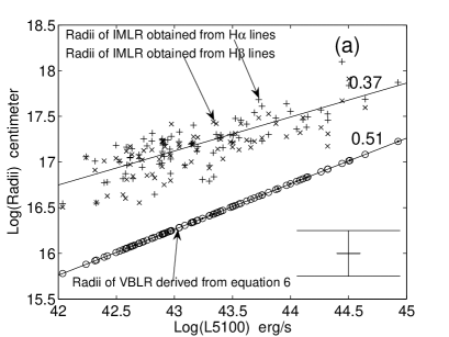
Figure 7: Correlation of the radii of IMLR and VBLR with black hole mass. Circles are the VBLR radius, $\times$ represent IMLR radius derived from H$\beta$ lines and $+$ from H$\alpha$ lines. Circles filled with dots represent the objects missing the IMGC. The radius of the VBLR is obtained from the $R_{\rm{BLR}}\sim$L5100 (equation 3) relationship on the top figure. These correlations supports a scenario of hierarchical evolution of AGNs. The typical uncertainty is plotted in the corner.

The evolution of $R_{\rm{VBLR}}$ and $R_{\rm{IMLR}}$ with luminosity and black hole mass are shown in Fig.7. The radius of the IMLR increases more slowly than VBLR with black hole mass and luminosity. The two emission regions have a trend to merge into one with higher luminosity or larger black hole mass; it is consistent with the emission lines’ behavior as shown in section 3.4. The points which represent objects with zero IMGCs also mainly lie on the large mass and large luminosity side. The slopes of these relations will be discussed in Section 4.4. Although most of the H$\alpha$ lines still need two Gaussian components to fit, there are three of them which only need one Gaussian component in our sample. The two Gaussian components in H$\alpha$ lines also show a trend to merge into one single Gaussian component with FWHM becoming larger, though the trend is not as obvious as for H$\beta$ lines. Once again the systematically different trends of evolution of $R_{\rm{VBLR}}$ and $R_{\rm{IMLR}}$ are consistent with our assumption that they are physically two distinct emission regions.

4.2 Balmer decrement in different Gaussian components and stratified geometry of the IMLR

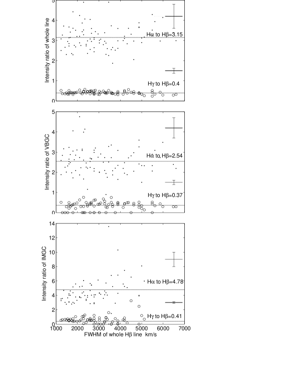
Figure 8: Dots represent intensity ratio of H$\alpha$ to H$\beta$ lines. Circles represent H$\gamma$ to H$\beta$ lines. The numbers marked in the figure are the averaged values. Typical uncertainty is plotted as a cross.

It is possible that density, temperature and geometric shape of the two regions (VBLR and IMLR) are different, then the collisional effect and different ionization energies of the three Balmer lines may cause different Balmer decrement in the two regions. Here we show the Balmer decrement of the whole line, VBGC and IMGC in Fig.8. There are two sources whose $\rm{H}\alpha$ or $\rm{H}\beta$ or both do not fit well with the double Gaussian model; these two points are excluded in Fig.8a when calculating the intensity ratio of $\rm{H}\alpha$ to $\rm{H}\beta$. Similarly, there are sixteen sources whose $\rm{H}\beta$ or $\rm{H}\gamma$ or both do not fit well; these points are excluded when calculating the intensity ratio of $\rm{H}\beta$ to $\rm{H}\gamma$. The points excluded in Fig.8a are also excluded in Fig.8b and Fig.8c. In addition, fifteen sources’ $\rm{H}\gamma$ do not have broad Gaussian; these points do not appear in intensity ratio of H$\beta$ to $\rm{H}\gamma$ in Fig.8b. Fourteen sources’ $\rm{H}\alpha$ or $\rm{H}\beta$ or both only need a VBGC to fit (i.e., they do not have IMGC), so these sources are not included in Fig.8c when calculating the $\rm{H}\alpha$ to $\rm{H}\beta$ ratio. Similarly 22 sources’ $\rm{H}\beta$ or $\rm{H}\gamma$ or both only have VBGC, and are thus excluded in Fig.8c when calculating the $\rm{H}\beta$ to $\rm{H}\gamma$ ratio. In summary, there are 88, 88 and 76 points used to calculating H$\alpha$ to H$\beta$ ratio in Fig.8a, b and c, respectively; correspondingly, there are 74, 59 and 52 points in H$\gamma$ to H$\beta$ ratio.

In VBLR, H$\alpha$/H$\beta$ is 2.54 and H$\gamma$/H$\beta$ is 0.37, which is consistent with a pure H model with T=15000 K, Ne=$10^{10}$ cm^-3 (Krolik et al. 1978). In IMLR, H$\alpha$/H$\beta$ is 4.78, which is much higher than that in VBLR, consistent with previous results (Netzer & Laor 1993; Mullaney & Ward 2008). These can be caused by collisional effect which can lead to an effective emission increase for H$\alpha$ but not for H$\beta$ or H$\gamma$ (e.g. Osterbrock 1989). This result suggests a higher gas density in IMLR. It has also been argued that dust in the emission region can cause higher Balmer decrement (Binette et al. 1993). Therefore, it also suggests that IMLR may be contaminated by dust. On the other hand, the H$\gamma$ to H$\beta$ ratio is also slightly higher in IMLR (0.41) than that in VBLR (0.37). As H$\beta$ and H$\gamma$ are produced from similar process, the slightly higher H$\gamma$ to H$\beta$ ratio is not well understood.

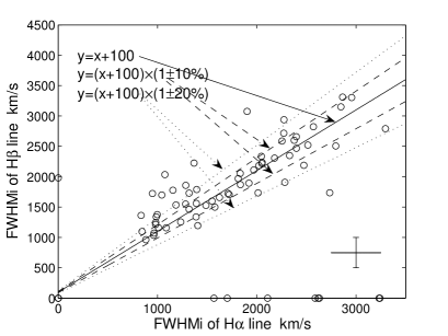
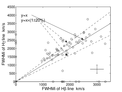
Figure 9: Correlations of between the three lines for the IMGC. Upper panel: between the H$\alpha$ and H$\beta$; Lower panel: between the H$\gamma$ and H$\beta$. The linear correlations between them indicates that the IMGCs for all these three lines originate from physically connected regions, even if not exactly from the same region. Typical uncertainty is plotted as a cross.

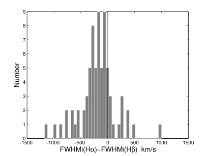
Figure 10: Distribution of FWHM differences between the three lines for the IMGC. Upper panel: between the H$\alpha$ and H$\beta$; Lower panel: between the H$\gamma$ and H$\beta$. The FWHM of H$\alpha$ and H$\gamma$ is offset systematically by around -200 km/s and +200 km/s around that of H$\beta$, respectively. This suggests a stratified geometry for the IMGC, where H$\alpha$, H$\beta$ and H$\gamma$ lines are produced at increasing radii respectively.

In Fig.9, we show the correlations between the first three Balmer lines for the IMGC, i.e., between the H$\alpha$ and H$\beta$ lines, and between the H$\gamma$ and H$\beta$ lines. The linear correlations between them indicates that the IMGCs for all these three lines originate from physically connected regions, even if not exactly from the same region. In Fig.10, we show the distributions of FWHM differences between the three lines for the IMGC. The FWHM of H$\alpha$ and H$\gamma$ is offset systematically by around -200 km s^-1 and +200 km s^-1 around that of H$\beta$, respectively. This suggests a stratified geometry for the IMLR, where H$\gamma$, H$\beta$ and H$\alpha$ lines are produced at increasing radii respectively. FWHM of the whole line, H$\alpha$ is also systematically larger than H$\beta$ (Greene & Ho 2005, Shen et al 2008). It is consistent with the RM result (Kaspi et al. 2000) which showed that radius of BLR obtained from H$\alpha$ is larger than that of H$\beta$ in most of the sources. Although there is no difference in the ionization degree of H$\alpha$, H$\beta$ and H$\gamma$, the above result can be explained that the inner skin of torus is the IMLR, therefore, it has more dust in the region with larger radius. There are mainly two processes. First, dust reddening will make the H$\gamma$ produced in the region much closer to the torus be extincted most seriously, the H$\beta$ will suffer less extinction and H$\alpha$ will be least extincted. Therefore the average radius of the H$\alpha$ region will be larger than H$\beta$ and H$\gamma$. Second, collisional excitation contributes a lot to H$\alpha$ line but not significantly to H$\beta$ and H$\gamma$ line, so the region much closer to the torus with a higher density will produce relatively more H$\alpha$. This also causes the FWHM of H$\alpha$ to be smaller than H$\beta$ and H$\gamma$.

4.3 Baldwin effect in Intermediate Gaussian component

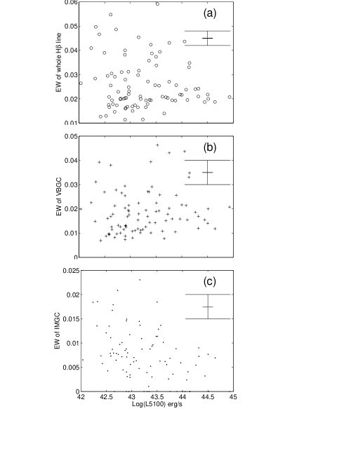
Figure 11: Correlation between equivalent width and continuum luminosity, based on the analysis of H$\beta$ lines. Slight Baldwin effect is shown in the IMGC (bottom plot) but not on the VBGC. Typical uncertainty is plotted as a cross.

The relation between the irradiation region and the central continuum is important, since the emission lines are thought to be mostly caused by photoionization. Fig.11 is plotted based on the analysis of H$\beta$ lines. Baldwin effect can be seen in the bottom plot. The Pearson Correlation Coefficient (PCC) is -0.39. We bootstrap it 100000 times and obtain 10 PCC larger than 0, so PCC is smaller than 0 at 99.99% confidence level. Pearson Rank Correlation Coefficient (PRCC) is -0.48, at 99.9% confidence level smaller than 0 using the same method as the confidence level calculation of PCC. However no Baldwin effect is seen in the top (Pearson correlation coefficient is -0.1) or in the middle plot (Pearson correlation coefficient is 0.1). It means that the Equivalent Width (EW) of the IMGC becomes smaller when the AGN becomes brighter, whereas the EW of the VBGC does not change with the continuum luminosity. This phenomenon has also been seen by Marziani et al. (2009). Since EW reflects the covering factor of the emission region, the above result supports the scenario that the VBLR is nearly spherical, but the IMLR has a flattened geometry. Therefore in the absence of other knowledge of other parameters of the gas, we can use the higher EW as a supportive (albeit not conclusive) evidence for a higher covering factor. There is also evidence that the dust torus has a smaller covering factor with higher luminosity (Wang et al. 2005). We therefore suggest that the cause of the slight Baldwin effect of IMLR can be the same, i.e., the innermost region of the dusty torus can be sublimated away by the strong irradiation of the AGN. Therefore we can infer that IMLR and VBLR have different geometries.

4.4 Location and Geometry of IMLR

Based on the above analysis, a picture of IMLR has emerged. In comparison with VBLR (the traditionally called “Broad Line Region” with a near spherical structure in virialization equilibrium), it has a larger radius and higher density, contains more dust, is more flattened, and is thus consistent as being the inner boundary region of the dust torus of AGN. As shown in Fig.7, the radii of both VBLR and IMLR are primarily determined by the continuum luminosity of the AGN. $R_{\rm{BLR}}$ obtained with equation (6) is used as the radius of VBLR there. Then $R_{\rm{IMLR}}\propto L^{0.37\pm 0.06}_{\rm{opt}}$ is derived from equation (3) as we have shown in Fig.7(a). The stratified geometry of IMLR, as inferred from Fig.10 in section 4.2, is also consistent with the above picture.

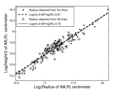
Figure 12: Dots and circles represent $h$ obtained from $R_{\rm{IMLR}}$ based on H_α and H_β separately; they have negligible differences. The height of the inner torus (IMLR) increases when its radius increases with an index smaller than unity.

The receding velocity of torus with luminosity can be also obtained from the analysis of type I AGN fraction. A relation between the covering factor $C$ and $L5100$ can be obtained from Maiolino et al. (2007): $\log{C}=-0.18\log{(\frac{L5100}{erg/s})}+7.4$, consistent with Wang et al (2005). If $R_{\rm{IMLR}}$ is used as the radius of the inner torus, then $C=4\pi\sin{\theta}=4\pi\frac{h}{h^{2}+R^{2}_{\rm{IMLR}}}$, and the height of the inner torus $h$ can be calculated from this relation, as shown in Fig.12. Clearly the relationship between $h$ and $R_{\rm{IMLR}}$ can be fitted with a power-law form. Since $C_{1}$ affects the index very weakly in this fitting, we just let $C_{1}=0$ in Fig.12. The height of the inner torus increases when its radius increases with the relation $h\propto R^{0.69}\propto L^{0.25}$, which controls the geometry of torus.

RM based on infrared emission is consistent with $R_{\rm{torus}}\propto L^{0.5}_{\rm{opt}}$ (Suganuma et al. 2006), which agrees with the prediction of a toy model for the sublimation process (Krolik & Begelman 1988). However, Suganuma et al. (2006) did not provide the index’ error of $R_{\rm{torus}}-L_{\rm{opt}}$ relation. We refit the data with error and the best fitting is $R_{\rm{torus}}\propto L^{0.46\pm 0.09}_{\rm{opt}}$, statistically consistent with our relation between IMLR radius and luminosity ($R_{\rm{IMLR}}\propto L^{0.37\pm 0.06}_{\rm{opt}}$).

However, the radius of IMLR that we calculated here is strongly dependent on the radius of VBLR, i.e., dependent on the $R_{\rm{BLR}}\sim L5100$ relation. If equation (5) is used to calculate the radius of BLR which is used as the radius of VBLR here, we would obtain $R_{\rm{IMLR}}\propto L^{0.53\pm 0.07}$, which is also consistent with the infrared RM result of $R_{\rm{torus}}\propto L^{0.46\pm 0.09}_{\rm{opt}}$. However, we prefer equation (6) because it has taken into account the correction of starlight (Bentz et al. 2006). Equation (6) is also consistent with a simple radiation pressured dominated VBLR where $L/R^{2}=$constant.

All of these analysis suggest that IMLR has roughly the same receding velocity as torus. Combined with the analysis in the sections above, we conclude that IMLR is the inner part of a dust torus.

4.5 Cartoon of the Broad Line Region evolution

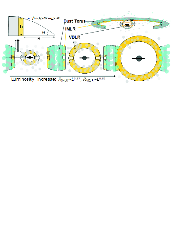
Figure 13: Cartoon of the Broad Line Region evolution. With increasing black hole mass and luminosity, both the VBLR and IMLR expand. The radius of VBLR increases faster, so the two regions have a trend to merge into one.

Based on the analysis above, a simple scenario of the BLR (BLR=VBLR+IMLR) evolution can be constructed as shown in Fig.13. The inner spherical region is the VBLR. It expands to a larger radius with luminosity increase and perhaps also black hole mass increase. We suggest that the IMLR is the inner part of the torus, which can be sublimated by the central radiation and thus its radius also increases with luminosity increase. Naturally the IMLR will be photoionized by the irradiation of the central AGN and the material gravitationally bound by the central black hole will be varialized with the gravitational potential of the central black hole, as determined by equations (1) and (2). Since the height of torus increases slower than the inner radius of the torus when luminosity increases, the covering factor of the IMLR decreases with luminosity (and larger radius) as shown in the cartoon. When the luminosity is high enough, the two regions may eventually merge into one. The observed broad emission line is thus the superposition of the emission from the two regions. When luminosity is large, the broad line region and torus become one single entity, but with different physical conditions. This scenario is consistent with the dust bound BLR hypothesis (Laor 2004; Elitzur 2006). Suganuma et al. (2006) also showed that the delay time of infrared emission is always longer than the delay time of emission lines of the corresponding AGN, but sometimes they are very close to each other and become almost the same. This is also consistent with the inner torus region as the origin of the IMGC.

5 Other supporting evidence for the two-components model

5.1 The micro-lensing result of BLR in J1131-1231

A piece of supportive evidence for the existence of IMLR comes from the study of the micro-lensing of the Broad Line Region in the lensed quasar J1131-1231 (Sluse et al. 2007, 2008). In this work they found evidence that the H$\beta$ emission line (as well as H$\alpha$) is differentially microlensed, with the broadest component (FWHM   4000 km/s) being much more micro-lensed than the narrower component (FWHM   2000 km/s). The emission line can be well decomposed into two components and the emission line’ profile has been significantly changed after microlensed compared to the original line. Because the amplitude of micro-lensing depends on the size of the emitting region, it can be naturally explained as the broadest component of the emission line comes from a more compact region than that of the narrower component. Although it can also be explained as a single region with a range of gas velocities at different radii, the explanation comes out from our model is natural.

5.2 The Mrk 79’ double peaks in CCCD map

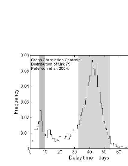
Figure 14: Cross Correlation Centroid Distribution of Mrk 79. The first peak is the usually used delay time range of broad line region which we take as the delay time of the VBLR. The second peak is the corresponding delay time range of the IMLR according to the FWHM ratio of their emission lines.

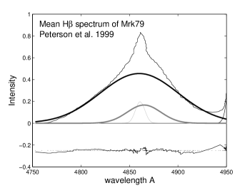
Figure 15: Decomposition of Mrk 79’s H$\beta$ line. The green line is the normal narrow line which we do not discuss here. The yellow line represents the IMGC with FWHM of 2522 km$\cdot s^{-1}$, and the blue line represents the VBGC with FWHM of 5856 km$\cdot s^{-1}$.

Then, we turn to the RM experiment. If the IMLR is really a physically distinct emission region apart from the VBLR, another peak corresponding to the radius of this region might appear in the cross correlation function between the lightcurves of the emission line and the continuum. In fact, a possible example exists in the database of RM observations (Peterson et al. 1998; 2004). Mrk 79 shows obviously double peaks in the cross correlation centroid distribution map as shown in Fig.14, which has not been explained well so far. There are four subsets of RM data for Mrk 79 which were taken in different time periods, and the double-peaked cross-correlation centroid distribution of Mrk 79 is from the fourth period. The measured time delays are about $9-16$ days in the subsets $1-3$ (Peterson et al. 2004), while in the 4th subset there are two typical time delays, one is about $6-10$ days which is consistent with subsets $1-3$, and the other is about $42$ days, as shown in Fig.14. Here we suggest that the shorter time delay, i.e. $6-10$ days, is the delay time of VBLR, which was also observed in subsets $1-3$. The longer time delay, i.e. $\sim 42$ days, is possibly the delay time of IMLR, which was only observed in the fourth subset. The mean H$\beta$ spectrum of Mrk 79 can be well described in a three Gaussian component model (Peterson et al. 1999), i.e., a normal narrow line, an IMGC and a VBGC, as shown in Fig.15. Based on the simple relation in section 4.1 (equation 3), we get $R_{\rm{IMLR}}/R_{\rm{VBLR}}=V^{2}_{\rm{VBLR}}/V^{2}_{\rm{IMLR}}=(5856\rm{km/s}/2522\rm{km/s}))^{2}=5.4$. Therefore the delay time for IMLR should be 32-54 days, fully agrees with the second peak of CCCD. This agreement also suggests that our rather arbitrary choice of $C_{0}=f_{1}/f_{2}=1$ does not deviate from its true value significantly, at least not for Mrk 79. However, it should be noted that in the mean H$\beta$ the VBGC dominates over the IMGC, but in the CCCD the second peak appears to be much stronger. Probably, in the fourth subset, the IMLR responses to the continuum more than the VBLR, i.e., the IMGC is more variable.

On the other hand, for the majority of other sources with RM observations, the IMGC is not important. We re-examined the ten RM sources with public data on Peterson’ website. Six of them only need one Gaussian component to describe the broad line of H$\beta$, one of them has double peak profile and one has irregular profile, only two of them need VBGC+IMGC to fit. In addition, 90% of the sources that plot on the R-L relation (Kaspi et al 2005) has luminosity larger than $10^{43}$ erg s^-1 and more than 60% larger than $10^{44}$ erg s^-1, which prefers the emission line to be one single Gaussian profile (In our sample, there are 14 sources’s H$\beta$ only need one Gaussian component, 11 of them has luminosity larger than $10^{43}$ erg s^-1 and 6 of them larger than $10^{44}$ erg s^-1 ). Therefore the Radius-Luminosity relationship established in emission line RM measurements may be valid only for the VBLR, i.e., the R-L relation only gives the radius of VBLR, as assumed in section 4.1. This is probably why we did not see double peaks in most of the CCCD maps (As shown above, even for Mrk 79, the two peaks were obtained in only one observation period out of four periods in total.). Two of the sources with double Gaussian line profiles are NGC 4051 and Mrk 509; the lag times for the two components of both sources satisfy this simple relationship $t_{\rm{IMLR}}/t_{\rm{VBLR}}=V^{2}_{\rm{VBLR}}/V^{2}_{\rm{IMLR}}$, consistent with our two-components BLR assumption. Interestingly the lag time for the VBGC of NGC 4051 is between 1 to 2 days, significantly different from the lag time of about 4 days for the whole line. This revised lag time makes NGC 4051 consistent with the Radius-Luminosity relationship in equation (5) or (6), resolving the outstanding problem on the significant deviation of NGC 4051 from the Radius-Luminosity relationship (Kaspi et al. 2005). The detailed results on our re-analysis of the RM data with this two-components model will be presented elsewhere (Zhu & Zhang 2009).

5.3 The narrower RMS spectra

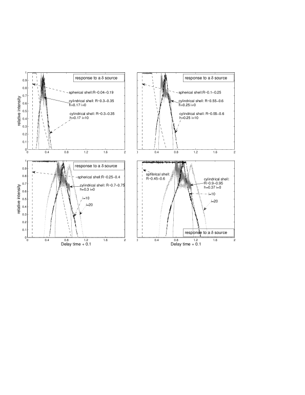
Figure 16: Different responses of different geometries to a delta impulse. Time is normalized to arbitrary unit. Each figure shows a different $R_{\rm IMLR}-R_{\rm VBLR}$ pair

We propose that the VBLR and IMLR are identified with the variable regions that scales with luminosity. If this is the case, one might expect that the VBGC would vary more than the mean spectrum as it has smaller radius. However, that is not observed; the RMS spectrum of the emission line is normally (but not always) narrower systematically than the mean spectrum (Collin et al. 2006). In our model, IMLR has a flattened geometry, and our simulations show that it can create a narrower response function to a delta impulse even with radius much larger than the VBLR. We carried out a straightforward test by calculating the responses of the two components to the continuum. In this simple geometrical model, the VBLR is a spherical shell and the IMLR is a cylindrical shell (representing a flattened disk-like geometry with inner and outer boundary). The gas density inside each region is independent of radius, i.e., the gas distribution could be clustered, but the distribution of gas clusters is independent of radius. The thickness of the VBLR shell is chosen to be three times that of the IMLR, because the VBLR is thought to have much lower density. The emissivity law of the two emission line regions is chosen in such a simple way that the emission line flux is proportional to the density times the continuum flux received at any point in the two regions. This means that the broad emission line intensity is proportional to the covering factor of each region. The line profile at any radius is assumed to have a Gaussian profile, with velocity determined from equation (3). The overall broad emission line from each region is thus the superposition of all broad lines from all radii. The response functions with different combinations of parameters for the two shells and the inclination angle of IMLR are shown in Fig.16. It can be seen that the IMLR normally can produce a narrower response function when the inclination angle is not very large. A narrower RMS spectrum can be easily calculated based on the narrower response function of IMLR. However, the FWHM difference in modeled RMS and mean spectra is not as significant as the observed. The simulation is carried out with noiseless, evenly sampled data, so further work is needed to see if this model can explain the narrower RMS spectrum quite well. In any case, the narrower RMS is not in conflict to our model of two distinct broad line regions, with the outer region has a flattened geometry. The requirement for small inclination angles simply suggests that most of the reverberation mapped objects have small inclination angles, a generic property of AGNs with broad emission lines. Further more extensive calculations on the detailed responses of the two broad line regions to characteristic continuum light curves of AGNs and comparisons with data will be presented in a future work (Zhu & Zhang 2009).

6 On the two problems of AGNs

6.1 The under-massive black hole problem of NLS1s

RM-based black hole mass is calculated by the virial equation

$$M_{\rm{BH}}=\frac{R_{\rm{BLR}}}{G}f^{2}\rm{FWHM}_{\rm{H}\beta}^{2},$$ (7)

where FWHM_Hβ is the FWHM of the whole H${\beta}$, which represents the virial velocity of the BLR. For an isotropic velocity distribution, as generally assumed, $f=\sqrt{3}/2$ (Onken et al. 2004). $R_{\rm{BLR}}$ is the BLR radius that can be calculated from equation (5) or (6). As assumed in section 4.1 and further discussed in section 5.2, the radius obtained from RM may represent the radius of the VBLR actually. If we take this assumption, FWHM of the VBGC, instead of FWHM of the whole line, should be used to calculate the black hole mass. We therefore correct the black hole mass in this way,

$$M_{\rm{BHb}}=\frac{R_{\rm{VBLR}}}{G}f^{2}\rm{FWHM}^{2}(\frac{\rm{FWHMb}}{\rm{FWHM}})^{2},$$ (8)

where FWHMb is the FWHM of the VBGC, and $R_{\rm{VBLR}}$ is taken as the $R_{\rm{BLR}}$ in equation (5) or (6). It gives a more significant mass correction for NLS1s than for BLS1s as shown in Fig.17(a). The correction factor is near unity when FWHM reaches about 5000 km$\cdot$s^-1. We use L5100 as an indicator for continuum luminosity, and a correction for accretion rate has also been shown in Fig.17(c). After such correction, NLS1s still have smaller black hole masses but normal accretion rate in units of the Eddington rate.

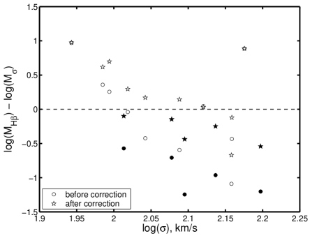
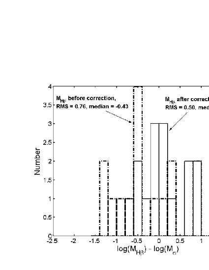
Figure 18: Comparison between black hole mass measured here and that predicted by the currently used M-sigma relation $M\propto\sigma^{4}$ (Tremaine et al. 2002), for fifteen sources in our sample with dispersion measurements (Shen et al. 2008). Upper panel: Circles represent those with black hole masses obtained with FWHM of the whole line used. Pentagrams represent those with corrected black hole mass. Filled symbols are NLS1s. Lower panel: Histogram of the mass ratios before and after the correction. After the correction, the median value of $(\log M_{{\rm H}\beta}-\log M_{\sigma})$ is much closer to zero, and the dispersion is reduced from 0.76 to 0.50 dex.

Fifteen objects in our samples have velocity dispersion measurement data (sigma) in Shen et al. (2008), as shown in Fig.18, where comparisons are made between black hole masses measured here and that predicted by the currently used M-sigma relation $M\propto\sigma^{4}$ (Tremaine et al. 2002). It is obvious that the masses of all NSL1 (filled symbols in the upper panel of Fig.18) are well below, but become more very close to, the predictions of the M-sigma relation before and after the correction, respectively. For other AGNs no significant changes to their masses are introduced by the correction process. As shown in the lower panel of Fig.18, after the correction, the median value of $(\log M_{{\rm H}\beta}-\log M_{\sigma})$ is much closer to zero, and the dispersion is reduced from 0.76 to 0.50 dex, which is consistent with the black hole mass uncertainty of 0.5 dex in RM (Peterson 2006). The effect of the correction is obvious, albeit small number statistics due to the limited sample.

6.2 The under-populated luminous type II problem of Seyfert galaxies

It has been shown that the receding torus model with constant torus height fails to provide a good fit to the data of type II AGN fraction as a function luminosity, and a good fitting can be given when $h$ increases slowly with luminosity with the relation $h\propto L^{0.23}$ (Simpson 2005), in excellent agreement with that of IMLR as we have shown in section 4.4. Note that here we consider the change of covering factor is totally because of the change of the opening angle during the calculation, following Wang et al. (2005). This agreement suggests that the receding of torus is sufficient to explain the decrease of covering factor with decreasing luminosity. Our model is consistent with the torus that Simpson (2005) needed to explain under-populated luminous type II AGNs.

7 Conclusion and discussion

We conclude that the decomposition of broad H$\beta$, H$\alpha$, and H$\gamma$ line of the AGNs confirms the two component model of BLR which has been suggested by several previous studies (e.g., Brotherton 1996; Sulentic et al. 2000; Hu et al. 2008.). We have made detailed analysis about the two emission regions (VBLR and IMLR) based on the Balmer line decomposition, and find other supportive evidence for this model. Our main conclusions are:

1. The two Gaussian components exhibit evolutions with increasing FWHM (we note in passing that because the two components show quite different dependence with FWHM and luminosity as to be shown in the following, we rule out the possibility that the dependence is caused by systematic biases in the decomposition process). The evolution is much stronger for the H$\beta$ and H$\gamma$ lines. Our results offer strong evidence of the evolution of the broad line region (consists of a IMLR and a VBLR) evolution from NLS1s to BLS1s. We obtain the luminosity dependence for the radius of IMLR, $R_{\rm IMLR}\propto L^{0.37}$, if the luminosity dependence for the VBLR is taken as $R_{\rm VBLR}\propto L^{0.52}$ (Kaspi et al. 2005). The two emission regions have a trend to merge into one region with luminosity increasing. Balmer decrement and the Baldwin effect in IMLR indicate that it has a flattened geometry, higher density and contains more dust, compared to the VBLR. The receding velocity of IMLR is consistent with dust torus. Therefore, we suggest the IMLR is the hot inner skin of torus. A cartoon of the evolution of BLR emerge from these analysis.

2. There are other evidence in support of this two component model. The study of micro-lensing provides possible evidence for the existence of IMLR. The double-peaked CCCD from the RM data of Mrk 79 also provides possible evidence. Simulations suggest that the narrower RMS spectra of broad emission lines from many AGNs may be consistent with our model, although more work needs to be done to establish this as the case. The existence of a weak IMGC in the broad emission lines of many sources with RM measurements may cause systematic biases for the measurements of the radius of the VBLR, thus biasing the Radius-Luminosity relation for the VBLR. It will be helpful to decompose each broad emission line into two Gaussian components as we have done here, and then do cross-correlation analysis between the continuum and each of the two components, in order to measure the Radius-Luminosity relations for the two components independently.

3. In our model, only the VBGC should be used to estimate the black hole mass, and the radius measured by reverberation mapping based on emission lines normally represents the radius of this region. After correction for black hole masses, NLS1s still have smaller black hole masses (compared to BLS1s) but normal accretion rate in units of Eddington rate. Therefore, the black hole mass increases from NLS1s to BLS1s by following the M-sigma relation established for normal galaxies.

   We obtain the luminosity dependence for the height of IMLR as $h\propto L^{0.25}$. It can well explain the luminosity function of AGN, if the decreasing fraction of type II AGNs for higher luminosity is due to completely the decreasing covering angle of the dusty torus to the central irradiation source (Simpson. 2005).

   Therefore both the problem of under-massive black hole in NLS1s and the problem of under-populated luminous type II Seyfert galaxies can be understood properly if our model is true, still more concrete evidences for this model are needed.

Hu et al. (2008) found evidence that IMLR is related to inflow towards the VBLR. Combining with this conclusion, we suggest that the inflow from the inner boundary region of AGN’s dusty torus may provide the supply to the accretion disk surrounding the central black hole. The strong and positive luminosity dependence of the geometry of IMLR suggests that the dust sublimation by the central accreting black hole’s radiation dominates the structure and evolution of IMLR. If IMLR is related to inflow (Hu et al. 2008), we may be able to further suggest that the inflow is caused by the dust sublimation, i.e., a consequence of the feed-back of the black hole’s accretion and radiation. Because IMLR is also ionized similarly to VBLR, the IMLR induced viscosity allows efficient angular momentum transfer to drive gas inflow from the dust torus and consequently fuel the accretion flow onto the central black hole. In this scenario, the accretion flow is self-regulated by the radiation from the accretion disk through irradiation to the dust torus. Therefore the growth of the supermassive black hole is at the expense of consuming the material in the dust torus during the AGN phase; this is consistent with the observation that for very low luminosity AGNs, the luminosity decreases with decreasing absorption column, i.e., the AGNs in their last stages are running out accretion material supplied by the torus (Zhang & Soria et al. 2009). Of course not all material in the accretion flow falls into the black hole horizon to increase the black hole’a mass, since accretion winds and outflows are common in AGNs.

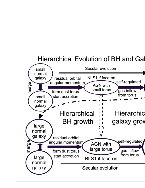
Figure 19: Illustration of hierarchical evolution of black hole, torus and host galaxy. Two galaxies merge to form a dust torus, due to the residual orbital angular momentum of the two galaxies in a binary. The dust torus is sublimated by the irradiation of the accretion disk around the central black hole. The gas produced by the sublimation process is ionized also by the irradiation of the accretion disk around the central black hole. The MRI viscosity in the ionized gas transfers the angular momentum outwards and thus fuels the accretion flow onto the central black hole; this is the AGN phase of a galaxy. Such self-regulated process grows the black hole by consuming the dust material in the torus, until the torus disappears and the AGN activity is turned off, i.e., a normal, inactive and larger galaxy is formed. In this scenario, NLS1 galaxies are the AGN phase (viewed through the opening cone of the dust torus) resulted from the merger of two smaller (dwarf) galaxies. Subsequent mergers of larger galaxies progressively produce AGNs with larger tori, higher luminosity and more massive black holes, in a hierarchical evolutionary sequence. It should be noted that here we only illustrate the processes of major mergers, in order to emphasize our main points, despite that fact that minor mergers are more frequent.

After the material in the dust torus is completely consumed, the AGN phase will be turned off and the galaxy becomes a normal and inactive galaxy. Indeed many AGNs in low luminosity (because of low accretion rate and low radiation efficiency) show very little, or even no signs of torus and/or broad line region; there is also no evidence for dust torus or broad line region in the centers of normal and inactive galaxies, including the Milky Way. Therefore the AGN’s dust torus is the missing link or bridge between the coeval growth of a black hole and its host galaxy. This would require that during the merging of two galaxies, a dust torus is first formed, perhaps due to the residual orbital angular momentum of the two galaxies. The dust torus then fuels the accretion and growth of the supermassive black hole through the self-regulation of irradiation to the dust torus by the accretion disk. The initial trigger to this self-regulation process may be Bondi accretion of gas with negligible angular momentum, or the low level AGN activities of the two black holes in the two parent galaxies before the merger. This evolutionary scenario is illustrated in Fig.19.

The above scenario is generally consistent with that proposed by Wang & Zhang (2007), but also with some important difference. We suggest that the torus is formed by the merging of two galaxies and disappears after each AGN cycle; the different appearance (mainly geometry) of torus in different types of AGNs are mostly due to the self-regulation of the accretion and irradiation of the AGN. Therefore in our scenario, torus evolution is fast (only lasting for one episode of AGN activity) and synchronized with that of the broad line region, whose evolution is also dominated by the luminosity of the AGN. Our torus evolution is mostly hierarchical. For example, although NLS1s also have generally smaller black hole masses, we do not find NLS1s deviate from the M-sigma relation more than the BLS1s after black hole mass correction made here. Therefore in our scenario NLS1s are produced by mergers of smaller galaxies compared to BLS1s; NLS1 may or may not show up as BLS1s in the future, depending upon if more galaxy mergers grow them up in the future. In the scenario of Wang & Zhang (2005), NLS1s are in their early growth stage and will grow to become BLS1 during this particular AGN cycle. Therefore their torus evolution is mostly secular. In practice, both hierarchical and secular evolutions should be needed for the black hole, torus and host galaxy. It is natural that hierarchical evolution dominates at high redshifts where merger rate is very high, and secular evolution dominates at low redshifts.

Table 1: Source properties and decomposition parameters. L5100 are given in units of $10^{42}$ erg $\rm{s}^{-1}$, ${M}_{\rm{BH}}$ are expressed in $10^{5}$ ${M}_{\sun}$. (1): Object name; (2): redshift; (3): L5100; (4): $M_{\rm{BH}}$; (5): Hb (height of the VBGC); (6): Hi (height of IMGC); (7): FWHM; (8): FWHMb; (9): FWHMi; (5), (6), (7), (8), (9) are parameters of H$\alpha$ lines; (10), (11), (12), (13), (14) are the corresponding parameters of H$\beta$ lines; (15), (16), (17), (18), (19) are the corresponding parameters of H$\gamma$ lines.

					H$\alpha$ lines					H$\beta$ lines					H$\gamma$ lines
NO	(1)	(2)	(3)	(4)	(5)	(6)	(7)	(8)	(9)	(10)	(11)	(12)	(13)	(14)	(15)	(16)	(17)	(18)	(19)
1	SDSSJ1152-0005	0.275	77.88	208.85	18.9	0	3610	3579	0	13.6	0	3640	3601	0	4.26	2.15	2529	3913	1493
2	SDSSJ1157-0022	0.178	140.86	1241.78	75.2	58.5	4844	6926	3241	48.56	0	6602	6598	0	15.7	5.77	4689	6627	2301
3	SDSSJ1307-0036	0.188	48.84	149.05	26.9	36.9	1873	3770	1285	11.3	8.45	2838	3793	1857	7.24	2.76	3023	4143	1597
4	SDSSJ1059-0005	0.283	92.33	224.16	16.2	24.4	1965	3839	1368	8.17	5.66	3208	4109	2224	5.8	0	4010	4362	0
5	SDSSJ1342-0053	0.129	23.61	293.32	14.3	27.8	2925	5767	2272	7.43	6	4195	6041	2716	3.43	3.39	3763	6445	2840
6	SDSSJ1307+0107	0.26	183.28	1056.59	40.6	28.1	4433	6240	2864	16.4	8.38	4874	5784	3311	11.4	0	4380	4851	0
7	SDSSJ1341-0053	0.17	32.02	97.72	22.9	57.5	2285	4490	1835	12.4	14.1	2653	4173	1869	6.15	8.04	2406	4791	1853
8	SDSSJ1344+0005	0.276	113	1133.83	31.1	24.9	5027	6849	3541	18.8	0	6478	6396	0	7.38	0	4751	5269	0
9	SDSSJ1013-0052	0.327	324.69	2732.11	38.1	0	4342	4257	0	23.1	0	4627	4623	0	11.1	0	4504	4937	0
10	SDSSJ1010+0043	0.237	…	…	…	…	…	…	…	…	…	…	…	…	…	…	…	…	…
11	SDSSJ1057-0041	0.087	5.28	42.13	7.78	51.8	2148	4946	1921	8.43	17.9	2468	5342	1894	4.84	10.3	2406	4028	2211
12	SDSSJ0117+0000	0.245	33.58	124.96	27.5	34.6	1828	3547	1185	13.1	8.99	2653	3801	1533	5.59	4.3	2591	4248	1853
13	SDSSJ0112+0003	0.074	4.16	32.75	15.4	41	1873	4566	1487	7	10.2	2221	4318	1527	0	9.48	1789	0	1923
14	SDSSJ1344-0015	0.141	30.36	78.27	24.5	68.4	1919	3881	1550	12.9	23.6	2097	3643	1598	7.85	10	2344	4208	1826
15	SDSSJ1343+0004	0.114	25.02	57.24	27.5	71	1736	3639	1391	10.9	25.9	1974	3997	1559	7.58	10.8	1974	3059	1633
16	SDSSJ1519+0016	0.233	100.02	628.19	35.6	16.8	3884	5251	2109	16.1	0	4874	4793	0	7.32	0	4010	4481	0
17	SDSSJ1437+0007	0.179	74.76	146.48	21	63.6	1965	4012	1631	11.7	22.7	2406	4315	1877	8.27	2.21	3578	4377	2278
18	SDSSJ1659+6202	0.31	210.04	752.96	16.9	36.1	3564	5479	2955	12.9	8.59	4319	5154	3303	4.88	10.9	2776	3989	2655
19	SDSSJ0121-0102	0.36	439.86	724.5	18.5	50.4	2833	4770	2377	14.6	15.4	3393	4688	2599	26.4	0	4134	4506	0
20	SDSSJ1719+5937	0.174	137.49	946.25	117	60.5	4936	6088	3232	56.2	0	5615	5550	0	12.2	0	3640	4077	0
21	SDSSJ1717+5815	0.279	208.76	511.13	38.6	25.6	2925	3814	1902	14.4	14.5	3578	4109	3076	7.64	0	3023	3381	0
22	SDSSJ0037+0008	0.362	277.83	369.99	33.2	55.2	1416	3424	948	14.7	6.71	2961	3801	1724	3.2	1.48	3332	4224	1708
23	SDSSJ2351-0109	0.252	64.75	246.21	10	11.8	3107	4733	2283	5.98	3.64	3640	5137	1907	0	18.6	2159	0	2382
24	SDSSJ2349-0036	0.046	2.13	35.98	27.2	72	2468	4222	2053	16.7	20.6	3023	4623	2236	4.84	5.69	3702	6560	2929
25	SDSSJ0013+0052	0.239	128.04	639.96	16.4	34.8	3427	5892	2795	12.3	7.01	4195	5423	2505	13.7	17	2838	4258	2418
26	SDSSJ1720+5540	0.055	19.96	175.4	64.5	78.7	4021	5098	3296	39.8	22.5	4134	5085	2790	7.96	3.14	2838	3607	1697
27	SDSSJ0256+0113	0.081	6.76	104.17	26.2	22	3336	4251	2474	13.9	4.93	3887	4623	2188	23.2	0	5121	5676	0
28	SDSSJ0135-0044	0.335	845.06	2960.01	101	19	4981	5451	2588	46.6	0	5861	5850	0	5.63	5.91	2714	4023	1963
29	SDSSJ0140-0050	0.146	22.95	107.38	23.9	38.7	2148	4241	1577	13.5	13.6	2776	4623	1499	9.19	0	4380	4792	0
30	SDSSJ0310-0049	0.206	57.01	471.05	24.9	45.7	3245	5174	2617	23.7	0	4997	4900	0	3.73	3.04	2776	3913	2123
31	SDSSJ0304+0028	0.368	120.96	306.39	19.6	0	3153	3066	0	8.99	1.83	3455	3595	1980	4.37	4.78	3023	5507	2346
32	SDSSJ0159+0105	0.198	37.36	188.85	12.4	41.2	2605	6198	2179	7.88	11.4	3270	6288	2305	7.99	0	3270	3568	0
33	SDSSJ0233-0107	0.177	26.13	184.98	22.5	40.8	2605	4514	2046	11.3	7.13	3578	4472	2335	…	…	…	…	…
34	SDSSJ0250+0025	0.045	2.07	9.93	18.6	94.1	1188	3439	981	9.84	28.2	1542	3801	1214	0	16.6	1542	0	1634
35	SDSSJ0409-0429	0.081	41.92	213.82	54.9	203	2650	5935	2254	28.9	58.7	3270	5576	2588	17.3	17.8	3270	5870	2463
36	SDSSJ0937+0105	0.108	14.45	63.25	20.7	98.4	2102	4946	1813	11.7	32.8	2468	5342	1969	5.64	17.8	2406	4028	2345
37	SDSSJ0323+0035	0.186	318.83	323.42	109	216	2239	4416	1710	54.9	84.1	2406	4841	1725	37.1	21.5	2714	4016	1617
38	SDSSJ0107+1408	0.216	56.76	120.52	28.6	54.7	1416	3194	1043	13.9	9.74	2591	3493	1699	4.76	6.17	2468	4678	1944
39	SDSSJ0142+0005	0.077	1.73	5.59	6.31	34.7	1051	3424	882	4.19	13.2	1234	3698	962	2.41	5.99	1419	3683	1251
40	SDSSJ0306+0003	0.095	3.14	12.56	14.1	39.2	1096	3262	844	5.99	8.83	1666	3595	1097	1.79	3.88	2159	4028	1897
41	SDSSJ0322+0055	0.09	6.44	33.31	18.9	56	1142	3442	917	4.86	10.9	2097	3801	1699	…	…	…	…	…
42	SDSSJ0150+1323	0.037	8.78	227.13	127	76.3	3473	5450	1703	45.07	0	5985	5949	0	19.7	0	4010	4488	0
43	SDSSJ0855+5252	0.069	5.81	23.72	31.7	109	1051	2739	834	12.5	20.7	1789	3082	1363	0	15.1	1542	0	1591
44	SDSSJ0904+5536	0.039	1.09	20.98	20.9	33.8	1828	3354	1389	9.34	7.07	2653	3801	1646	…	…	…	…	…
45	SDSSJ1355+6440	0.051	9.14	23	110	225	1325	2843	1010	54.6	87.1	1604	3063	1157	25.2	36	1666	2720	1405
46	SDSSJ0351-0526	0.075	31.62	120.58	83.7	255	2422	4566	2022	54.3	113	2776	4620	2183	0	76.9	2529	0	2831
47	SDSSJ1505+0342	0.058	7.98	18.08	23.2	98.9	1416	3887	1233	12.4	32.6	1604	4077	1254	8.47	14.3	2036	3309	1727
48	SDSSJ1203+0229	0.093	35.99	171.89	56	124	2559	4718	2051	41.9	27.2	3332	4392	2216	10.6	21.6	2961	5409	2704
49	SDSSJ1246+0222	0.078	45.44	170.3	41.3	148	2650	4870	2330	30.2	46.4	3023	4520	2348	16.4	27.3	2653	3875	2468
50	SDSSJ0839+4847	0.024	7.86	279.34	289	113	3976	5228	1568	130	0	5491	5428	0	63.9	0	4874	5327	0
51	SDSSJ0925+5335	0.087	5.44	17.86	7.9	36.8	1234	3757	1032	4.04	10.1	1666	4006	1272	…	…	…	…	…
52	SDSSJ1331+0131	0.048	11.05	26.69	41.9	172	1188	3294	987	25.6	61.7	1727	3698	1338	9.19	34.3	1480	4143	1312
53	SDSSJ1042+0414	0.08	7.41	38.49	7.82	51.3	2193	4946	2013	6.93	13.3	2283	4520	1734	0	11.8	2283	0	2428
54	SDSSJ1349+0204	0.033	2.48	45.98	111	220	2468	4908	1920	42.9	27	3455	5239	1558	…	…	…	…	…
55	SDSSJ1223+0240	0.072	8.15	59.21	35.8	27.9	1965	3044	1155	15	6.49	2776	3287	1777	11.5	0	2653	2959	0
56	SDSSJ0755+3911	0.034	7.88	26.39	58.2	164	1462	3321	1172	34.3	51.2	1912	3647	1344	…	…	…	…	…
57	SDSSJ1141+0241	0.047	3.37	26.76	27.4	53	1599	3576	1159	8.6	13.1	1789	3801	1221	…	…	…	…	…
58	SDSSJ1122+0117	0.04	4.94	17.08	45.6	144	1371	3298	1079	17	40.1	1604	3698	1235	…	…	…	…	…
59	SDSSJ1243+0252	0.077	4.31	9.24	13.8	84.3	1096	3292	961	6.56	29.6	1295	3287	1035	0	15.2	1295	0	1383
60	SDSSJ0832+4614	0.061	7.87	44.3	47.2	152	1965	5297	1624	24.3	44.9	2283	5342	1657	6.99	24.1	2776	6312	2588
61	SDSSJ0840+0333	0.053	4.57	124.7	40.9	0	3884	3805	0	15.5	0	4627	4551	0	10.2	0	2653	2920	0
62	SDSSJ1510+0058	0.036	21.63	365.27	212	276	3702	5935	2735	127	25.1	4874	5548	1735	31	48.1	3085	6675	2506
63	SDSSJ0110-1008	0.078	53.19	187.64	234	164	2102	3372	997	99.1	38.8	3085	3698	1376	59	0	3023	3288	0
64	SDSSJ0142-1008	0.031	20.11	266.31	416	256	3884	4946	2631	238	0	4380	4303	0	103	31.3	4134	5524	2405
65	SDSSJ1519+5908	0.069	7.95	15.03	25.8	122	1279	3337	1086	14	51.4	1419	3698	1157	0	26.1	1542	0	1681
66	SDSSJ0013-0951	0.074	3.86	8.08	9.59	53.5	1051	3216	899	4.61	18	1234	3493	1027	…	…	…	…	…
67	SDSSJ1535+5754	0.062	12.3	168.21	18.9	60.5	2970	5479	2569	14.3	17.4	3887	5959	2823	12.7	1.59	3085	3470	1732
68	SDSSJ1654+3925	0.042	3.6	35.71	36	155	2148	4490	1834	19.7	33.2	2591	4109	2054	0	23.2	2406	0	2562
69	SDSSJ0042-1049	0.058	3.89	33.23	20.4	69.7	1599	3757	1318	6.31	11.9	2283	4109	1729	6.51	2.04	2406	3377	650
70	SDSSJ2058-0650	0.09	4.15	28.15	13.6	51.4	1736	4598	1486	8.96	14	2097	5034	1420	0	23.7	3393	0	3752
71	SDSSJ1300+6139	0.052	9.25	214.11	67	49.3	3656	4948	2398	31.7	9.2	4504	5021	2657	1.43	4.69	1727	4834	1626
72	SDSSJ0752+2617	0.095	6.39	33.3	7.76	24.8	1599	4367	1283	4.35	7.55	2159	4726	1549	5.18	28	1480	4143	1430
73	SDSSJ1157+0412	0.082	14.61	28.9	53.9	163	1234	3325	982	25	55.9	1604	3647	1246	6.82	15.3	2221	3913	2064
74	SDSSJ1139+5911	0.085	15.6	77.92	17.9	58.8	2330	4718	1969	9.91	26.1	2591	5137	2110	…	…	…	…	…
75	SDSSJ1345-0259	0.028	4.39	65.57	18.4	144	2742	5859	2515	26.8	44.6	3332	6061	2521	0	38.6	2653	0	2969
76	SDSSJ1118+5803	0.061	25	275.2	334	215	3016	4362	1722	151	28.4	3887	4234	1706	88.4	0	3640	4036	0
77	SDSSJ1105+0745	0.074	7.83	253.4	24.6	46.3	3702	7001	2847	13.5	9.4	5121	7397	3150	2.57	8.4	2838	5754	2710
78	SDSSJ1623+4104	0.045	15.86	32.67	78.4	272	1645	3515	1388	56.9	126	1789	3801	1337	27.9	45.4	1851	3454	1571
79	SDSSJ0830+3405	0.07	21.87	454.94	75.2	84.6	4570	5859	3671	53.2	0	5491	5424	0	30.8	0	4874	5439	0
80	SDSSJ1619+4058	0.034	…	…	…	…	…	…	…	…	…	…	…	…	…	…	…	…	…
81	SDSSJ0857+0528	0.038	2.64	29.51	27.2	55.5	1828	3531	1394	8.26	14.7	2344	3801	1788	0	17.2	2036	0	2151
82	SDSSJ1613+3717	0.059	9.27	227.9	40.1	55.1	3336	5935	2399	21.6	8.94	4997	6370	2468	4.97	12.7	2529	6330	2301
83	SDSSJ1025+5140	0.062	9.42	34.11	47.3	96.9	1873	4617	1405	22.6	27.6	1912	4575	1194	5.56	16.2	2406	4258	2339
84	SDSSJ1016+4210	0.055	14.11	41.73	94.5	267	1645	3576	1318	44.6	112	1851	3904	1463	24	47.6	1789	3452	1572
85	SDSSJ1128+1023	0.051	10.94	16.71	99.5	248	1142	2601	880	39.7	64.7	1357	2783	974	…	…	…	…	…
86	SDSSJ1300+5641	0.072	13.98	54.01	54.5	83.1	1645	3151	1171	23.3	20.3	2221	3227	1494	…	…	…	…	…
87	SDSSJ1538+4440	0.041	3.79	66.77	15	41.8	2787	5859	2273	9.7	15	3763	5548	2938	0	11.8	2900	0	3165
88	SDSSJ1342+5642	0.073	4.99	52.18	34.7	35.6	1736	3120	1074	13.9	8.59	2776	3390	2034	0	10.4	2036	0	2276
89	SDSSJ1344+4416	0.055	8.3	17.68	41.7	113	1188	2961	964	26.1	49.7	1480	3185	1070	7.61	26.2	1419	3537	1300
90	SDSSJ1554+3238	0.049	17.46	384.87	60.4	82.8	4387	5859	3594	38	0	5491	5397	0	0	19.3	2653	0	2836

Figure 17: Black hole mass correction. X-axis is the FWHM of H$\beta$, y-axes are black hole mass, black hole mass correction factor and relative luminosity to $L_{\rm EDD}$ (Eddington Luminosity) from top to bottom. Black hole masses (in units of solar mass $M_{\sun}$) are plotted in logarithm scale. Circles are black hole mass and relative luminosity calculated with equation (1). Dots are that after correction using equation (4). Clearly the correction is more effective for AGNs with smaller FWHM, i.e., NLS1s. After the correction, their luminosity (in units of Eddington) appear to be in the same range, i.e., NLS1s do not show exceptionally higher luminosity. Typical uncertainty is plotted as a cross.

References

- Barger et al. (2005) Barger, A. J., Cowie, L. L., Mushotzky, R. F., Yang, Y., Wang, W.-H., Steffen, A. T., & Capak, P. 2005, AJ, 129, 578
- (2) Collin, S., et al. 2006, A&A, 456, 75C
- Greene & Ho (2006) Greene, J. E., & Ho, L. C. 2006, ApJ, 641, L21
- Bian & Zhao (2004) Bian, W., & Zhao, Y. 2004, MNRAS, 352, 823
- (5) Bentz, M.C., et al. 2006, ApJ, 644, 133
- (6) Binette, L., et al. 1993, ApJ, 414, 535
- (7) Bon, E., Popović, L.C̆, et al. 2006, NewAR, 50, 716
- Brotherton (1996) Brotherton, M. S. 1996, ApJS, 102, 1
- Collin et al. (2006) Collin, S., Kawaguchi, T., Peterson, B.M., & Vestergaard, M. 2006, A&A, 456, 75
- (10) Corbett, E.A., et al. 2003, MNRAS, 343, 705
- (11) Decarli, R., et al. 2008, MNRAS, 386, 15
- (12) Elitzur, M. 2006, in The Central Engine of Active Galactic Nuclei, ed. L. C. Ho & J.-M. Wang (San Francisco: ASP), 3
- (13) Elvis, M., et al., 1994, ApJS, 95, 1
- (14) Eracleous, M. & Halpern, Jules P. 2003, ApJ, 599, 886
- Ferrarese & Ford (2005) Ferrarese, L., & Ford, H. 2005, Space Science Reviews, 116, 523
- Gebhardt et al. (2000) Gebhardt, K., et al. 2000, ApJ, 539, L13
- (17) Goncalves, A.C., et al. 1999, A&A, 341, 662
- (18) Greene, J.E. & Ho, L.C. 2005, ApJ, 630, 122
- Grupe & Mathur (2004) Grupe, D., & Mathur, S. 2004, ApJ, 606, L41
- Hasinger (2004) Hasinger, G. 2004, Nuclear Physics B Proceedings Supplements, 132, 86
- Hasinger (2005) Hasinger, G. 2005, Growing Black Holes: Accretion in a Cosmological Context, 418
- (22) Hu, C. et al. 2008, ApJ, 683, L115
- (23) Joly, M. et al. 1985, A&A, 152, 282
- (24) Kaspi, S., et al. 2000, ApJ, 533, 631
- (25) Kaspi, S., et al. 2005, ApJ, 629, 61K
- (26) Kobayashi, Y., Sato, S., Yamashita, T., Shiba, H., Takami, H., 1993, ApJ, 404, 94
- Komossa & Xu (2007) Komossa, S., & Xu, D. 2007, ApJ, 667, L33
- (28) Komossa, S., et al. 2008, ApJ, 680, 926
- Komossa (2008) Komossa, S. 2008, Revista Mexicana de Astronomia y Astrofisica Conference Series, 32, 86
- (30) Krolik, J.H., et al. 1978, ApJS, 37, 459
- (31) Krolik, J. H. & Begelman, M. C. 1988, ApJ, 329, 702
- (32) La Mura, G., et al. 2007, ApJ, 671, 104
- Laor (2004) Laor, A. 2004, AGN Physics with the Sloan Digital Sky Survey, ASP Conference Series, 311, 169
- (34) Lawrence, A. 1991, MNRAS, 252, 586
- Magorrian et al. (1998) Magorrian, J., et al. 1998, AJ, 115, 2285
- (36) Maiolino, R., et al. 2007, A&A, 468, 979
- (37) Mason, K.O., et al. 1996, MNRAS, 283, L26
- (38) Marziani, P., et al. 2009, A&A, 495, 83M
- Marconi & Hunt (2003) Marconi, A., & Hunt, L. K. 2003, ApJ, 589, L21
- (40) Mullaney, J.R. & Ward, M.J. 2008, MNRAS, 385, 53
- (41) Nenkova, M. et al. 2008a, ApJ, 685, 147 (2008arXiv:0806.0511)
- (42) Netzer, H. & Laor, A. 1993, ApJ, 404, L51
- Onken et al. (2004) Onken, C.A., et al. 2004, ApJ, 615, 645
- (44) Osterbrock, D.E. Astrophysics of Gaseous Nebulae and Active Nuclei, 1989 University Science Books press, P 337-338.
- (45) Peterson, B.M., et al. 1998, ApJ, 501, 82
- (46) Peterson, B.M., et al. 1999, ASPC, 175, 41
- Peterson & Wandel (1999) Peterson, B. M., & Wandel, A. 1999, ApJ, 521, L95
- (48) Peterson, B.M., et al. 2004, ApJ, 613, 682
- (49) Peterson, B.M. 2006, Memorie della Societa Astronomica Italiana, 77, 581
- Peterson (2007) Peterson, B. M. 2007, in The Central Engine of Active Galactic Nuclei, ed. L. C. Ho & J.-M. Wang (San Francisco: ASP), 3
- (51) Popović, L.C̆, et al. 2008, RmxAC, 32, 99
- (52) Simpson, C. 2005, MNRAS, 360, 565
- (53) Sluse, D., et al. 2007, A&A, 468, 885
- (54) Sluse, D., et al. 2008, RMxAC, 32, 83
- (55) Strateva, Iskra V. et al. 2003, AJ, 126, 1720
- Steffen et al. (2003) Steffen, A. T., Barger, A. J., Cowie, L. L., Mushotzky, R. F., & Yang, Y. 2003, ApJ, 596, L23
- Steffen et al. (2004) Steffen, A. T., Barger, A. J., Capak, P., Cowie, L. L., Mushotzky, R. F., & Yang, Y. 2004, AJ, 128, 1483
- (58) Suganuma, M., et al. 2006, ApJ, 639, 46
- Sulentic et al. (2000b) Sulentic, J. W., Marziani, P., Zwitter, T., Dultzin-Hacyan, D., & Calvani, M. 2000, ApJ, 545, L15
- (60) Shen, J.J., et al. 2008, AJ, 135, 928
- (61) Tremaine, S., et al. 2002, ApJ, 574, 740
- (62) Ueda, Y., Akiyama, M., Ohta, K., & Miyaji, T. 2003, ApJ, 598, 886
- (63) Urry, C.M., & Padovani, P. 1995. PASP, 107, 803
- (64) Vestergaard, M. & Peterson, B.M. 2006, ApJ, 641, 689
- (65) Véron,P ., et al. 2002, A&A, 384, 826
- (66) Wang, J-M., et al. 2005, ApJ, 627, 5
- Wang & Zhang (2007) Wang, J.-M., & Zhang, E.-P. 2007, ApJ, 660, 1072
- Wang & Lu (2001) Wang, T., & Lu, Y. 2001, A&A, 377, 52
- Williams et al. (2004) Williams, R. J., Mathur, S., & Pogge, R. W. 2004, ApJ, 610, 737
- Zhou et al. (2006) Zhou, H., Wang, T., Yuan, W., Lu, H., Dong, X., Wang, J., & Lu, Y. 2006, ApJS, 166, 128
- Zhang et al. (2009) Zhang, Kai., Wang, Tinggui., et al. 2009, arXiv:0902.4390.
- (72) hang, W. M., Soria, R. Zhang, S. N. Swartz, D. A., Liu, J. 2009, accepted for publication in ApJ (arXiv:0904.1091)
- Zhu & Zhang (2009) Zhu, L., & Zhang, S.N. 2009, Science in China (G), in press (arXiv0907.1942Z)