Localized gap soliton trains of Bose-Einstein condensates in an optical lattice

Abstract

We develop a systematic analytical approach to study the linear and nonlinear solitary excitations of quasi-one-dimensional Bose-Einstein condensates trapped in an optical lattice. For the linear case, the Bloch wave in the $nth$ energy band is a linear superposition of Mathieu’s functions $ce_{n-1}$ and $se_{n}$; and the Bloch wave in the $nth$ band gap is a linear superposition of $ce_{n}$ and $se_{n}$. For the nonlinear case, only solitons inside the band gaps are likely to be generated and there are two types of solitons – fundamental solitons (which is a localized and stable state) and sub-fundamental solitons (which is a lacalized but unstable state). In addition, we find that the pinning position and the amplitude of the fundamental soliton in the lattice can be controlled by adjusting both the lattice depth and spacing. Our numerical results on fundamental solitons are in quantitative agreement with those of the experimental observation [Phys. Rev. Lett. 92, 230401 (2004)]. Furthermore, we predict that a localized gap soliton train consisting of several fundamental solitons can be realized by increasing the length of the condensate in currently experimental conditions.

I I. Introduction

Loading Bose-Einstein condensates (BECs) in an optical lattice formed by a laser standing wave has received increasing interest in the study of nonlinear atomic optics Barrett ; Orzel ; Cataliotti ; Greiner . Understanding the properties of BEC in an optical lattice is of fundamental importance for developing novel application of quantum mechanics such as atom lasers and atom interferometers 5 ; 6 ; 7 ; 8 ; 9 ; 9a ; 9b . Theoretically, some approximation methods are borrowed from solid state physics, which are used to investigate the dynamics of this system. It is mainly due to the fact that there are considerable resemblances between BEC droplet localized in an optical lattice and electron in a lattice. According to the theory of solid state physics, there exist band gaps between adjacent energy bands in the band structure of solid. In general, the energy bands exhibits spatially oscillating phenomena. As discussed in Refs. 10 and 11 , however, it is possible to generate soliton in the band gap when the nonlinearity compensates for atom dispersion caused by inter-site tunneling. The band gap soliton can be called gap soliton. The existence of the gap solitons was first predicted based on coupled-mode theory 12 , in analogy to optical gap solitons in Bragg gratings. Such a prediction was validated by a number of groups using some approximation approaches, such as tight binding approximation 10 , a complete set of on-site Wannier states 14 , an effective mass formula 15 and plane wave method 16 . Although they provide a convenient way to study the gap soliton of the BEC, the validity depends greatly on the nature of the underlying problem. From this point of view, it is desirable to develop a method that does not rely on above approximations 17 .

Strictly speaking, an accurate solution can be obtained by exactly solving the full nonlinear Schrödinger equation with a periodic potential. However, it is very difficult to derive analytical solutions because the full nonlinear Schrödinger equation is nonintegrable 18 . Consequently, some asymptotic approaches and numerical simulations are used to investigate this question. Using multiple scale method, Konotop and Salerno 17 predicted that bright solitons could come into being in a BEC with a positive scattering length and dark solitons could be stable with a negative scattering length. Subsequently, these predictions were proved by using asymptotic theories 19 ; 21 . Employing numerical simulations, Louis et al. 22 analyzed the existence and stability of spatially extended (Bloch type) and localized states of a condensate in the band gaps of the linear Bloch-wave spectrum.

Especially, Eiermann et al. 23 reported that gap soliton do neither move nor change their shape and atom numbers during propagation. That is to say, the gap soliton is pinned in an optical lattice without attenuation and change in shape. Such a soliton can be regarded as a spatially localized gap soliton, which is also called fundamental soliton in Ref. 37 . More importantly, localized bright solitons would be very useful for future applications, such as atomic interferometry 24 . Subsequently, some explanations to this observation were proposed by using numerical simulations (see Refs. 25 ; 26 ; 27 and references therein).

To better understand the characteristics of the linear and nonlinear solitary excitations of quasi-one-dimensional (1D) BECs trapped in an optical lattice, we develop a multiple scale method to derive analytically an explicit expression of the wave function. It is found that there are two types of gap solitons in the band gaps. One is fundamental soliton, which is always stable and pins a fixed position; the other is always unstable and decays gradually due to losing a part of its atoms. The paper is organized as follows: In Sec. II, we derive 1D amplitude and phase equations from the original three-dimensional Gross-Pitaevskii (GP) equation. Subsequently, by analyzing the stability regions of soliton formation, we obtain the formation condition of the fundamental solitons in the band gaps. A novel linear dispersion relation arising from the ground state and sound speed of this system in the band gaps are obtained in Sec. III. In Sec. IV, we develop a multiple scale method to study the nonlinear dynamics of the system. We derive a solution of the wave function and discuss its dynamical stability in the band gaps. It is found that the pinning position and amplitude of the fundamental solitons are controlled by adjusting both lattice depth and spacing. Furthermore, we propose an experimental protocol to observe a localized gap train consisting of several fundamental solitons in the condensate under currently experimental conditions. A brief summary is given in section V.

II II. EQUATIONS of AMPLITUDE AND PHASE

Based on mean-field approximation, the time-dependent GP equation of full BEC dynamics reads 16 ; 18 ; 22

$$i\hbar\frac{\partial\Psi}{\partial T}=[-\frac{\hbar^{2}}{2m}\nabla^{2}+V(X,Y,Z)+g|\Psi|^{2}]\Psi,$$ (1)

where $\Psi(X,Y,Z,T)$ is the order parameter of condensate, and $(X,Y)$ and $Z$ are the directions of strong transverse confinement and lattice. $N=\int dr|\Psi|^{2}$ is the total number of atoms, and $g=4\pi\hbar^{2}a_{s}/m$ is inter-atomic interaction strength with the atomic mass $m$ and the $s$-wave scattering length $a_{s}$ ($a_{s}>0$ represents the repulsive interaction). The combined potential $V(X,Y,Z)$ of the optical lattice and magnetic trap is

$$V(R^{2},Z)=E_{0}\sin^{2}(\frac{\pi Z}{d}) + \frac{1}{2}m(\omega^{2}_{\bot}R^{2}+\omega^{2}_{Z}Z^{2}),$$ (2)

$$\omega_{Z}\ll\omega_{\bot},$$

where $R^{2}=X^{2}+Y^{2}$, $E_{0}$ is the lattice depth. $d=\lambda_{L}/2$ is the lattice spacing, where $\lambda_{L}$ is the wavelength of laser beams. $\omega_{Z}$ and $\omega_{\bot}$ are frequencies of the magnetic trap in the axial $(Z)$ and transverse ($X$ and $Y$) directions, respectively. By introducing the dimensionless variables $t=\omega_{\bot}T$, $(r,z)=a^{-1}_{0}(R,Z)$ with transverse harmonic oscillator length $a_{0}=\sqrt{\hbar/m\omega_{\bot}}$, and $\psi=\sqrt{a^{3}_{0}/N}\Psi$, we obtain the following dimensionless GP equation

$$i\frac{\partial\psi}{\partial t}=-\frac{1}{2}\nabla^{2}\psi+[V_{0}\sin^{2}(\frac{\pi z}{D})$$

$$+\frac{1}{2}(r^{2}+\Omega^{2}z^{2})]\psi+Q|\psi|^{2}\psi,$$ (3)

where $V_{0}=E_{0}/(\hbar\omega_{\bot})$, $D=a^{-1}_{0}d$, $\Omega=\omega_{z}/\omega_{\bot}\ll 1$ and $Q=4\pi a_{s}/a_{0}$. Expressing the order parameter in terms of modulus and phase, i.e., $\psi=\sqrt{n}\exp(i\Phi)$, and then separating real and imaginary parts, we obtain

$$\frac{\partial n}{\partial t}+\nabla\cdot(n\nabla\Phi)=0,$$ (4)

$$\frac{\partial\Phi}{\partial t} + V_{0}\sin^{2}(\frac{\pi z}{D})+\frac{1}{2}(r^{2}+\Omega^{2}z^{2})+\frac{1}{2}(\nabla\Phi)^{2}$$ (5)

$$-\frac{1}{2\sqrt{n}}\nabla^{2}\sqrt{n}+Qn=0.$$

Equations (4) and (5) are (3+1)-dimensional, nonlinear and dispersive equations with a variable coefficient. To solve these equations, we introduce some reasonable approximations. Considering a ⁸⁷Rb condensate in a cigar-shaped trap with the frequencies of $\omega_{z}=2\pi\times 0.5$ Hz and $\omega_{\bot}=2\pi\times 85$ Hz 23 , we get $\Omega\approx 0.006$. The value of $\Omega$ is so small that the variation of the profile of the order parameter is slow in the $z$ direction. Thus, the wave function can be separated by $\psi(r,z,t)=G_{0}(r)\phi(z,t)$ with $\phi(z,t)=A(z,t)\exp[-i\mu t+i\varphi(z,t)]$. Here, the modulus and the phase are $\sqrt{n}=G_{0}(r)A(z,t)$ and $\Phi=-\mu t+\varphi(z,t)$ respectively. Owing to the strong confinement in the transverse direction, the spatial structure of function $G_{0}(r)$ can be well described by a solution of two-dimensional radial symmetric quantum harmonic-oscillator equation, i.e., $\nabla^{2}_{\bot}G_{0}+2G_{0}-r^{2}G_{0}=0$. The ground-state solution has the form $G_{0}(r)=C\exp(-r^{2}/2)$, where $C=1/\sqrt{\pi}$ can be found from the normalization condition $\int^{\infty}_{-\infty}|G_{0}|^{2}rdr=1$. Substituting them into Eqs. (4) and (5), we obtain

$$\frac{\partial A}{\partial t}+\frac{\partial A}{\partial z}\frac{\partial\varphi}{\partial z}+\frac{1}{2}A\frac{\partial^{2}\varphi}{\partial z^{2}}=0,$$ (6)

$$-\frac{1}{2}\frac{\partial^{2}A}{\partial z^{2}}+[\frac{1}{2}(\frac{\partial\varphi}{\partial z})^{2}-\mu+1+\frac{\partial\varphi}{\partial t}+$$

$$V_{0}\sin^{2}(\frac{\pi z}{D})]A+Q^{\prime}A^{3}=0,$$ (7)

with $Q^{\prime}=Q/(2\pi)=2a_{s}/a_{0}$. In order to obtain 1D amplitude and phase equations, we have multiplied Eq. (7) by $G^{*}_{0}$ and then integrated the resulting equation once with respect to the transverse coordinate to eliminate the dependence on transverse plane. An approach similar to this one has been widely used in quasi-1D (cigar-shaped) BEC problems 22 ; 28 ; 29 .

III III. LINEAR BLOCH MODES

We now consider a BEC trapped in a 1D optical lattice. Due to the strong confinement in the transverse direction, the system is similar to a wave guide, in which the excitation propagates in the elongated direction 31 . The strong confinement also ensures the dynamical stability of the linear excitation 31 . Therefore, we set $A=u_{0}(z)+\alpha(z,t)$ with $\alpha(z,t)=\alpha_{0}\exp(i\alpha_{1})+c.c.$ and $\varphi=\varphi_{0}\exp(i\alpha_{1})+c.c.$. Here, $c.c.$ is complex conjugate and $\alpha_{1}=kz-\omega t$. $k$ is the wave number and $\omega$ is the eigenfrequency. Without loss of generality, we assume $u_{0}(z)$ characterizing the condensate background. Considering that $\alpha_{0}$ and $\varphi_{0}$ are small constants, we obtain

$$i\omega\alpha_{0}=ik\varphi_{0}\frac{\partial u_{0}}{\partial z}-\frac{1}{2}k^{2}u_{0}\varphi_{0},$$ (8)

$$(\mu-1)u_{0}=-\frac{1}{2}\frac{\partial^{2}u_{0}}{\partial z^{2}}+V_{0}\sin^{2}(\frac{\pi z}{D})u_{0}+Q^{\prime}u^{3}_{0},$$ (9)

$$(\mu-1)\alpha_{0} = \frac{1}{2}k^{2}\alpha_{0}-i\omega\varphi_{0}u_{0}+V_{0}\sin^{2}(\frac{\pi z}{D})\alpha_{0}$$ (10)

$$+3Q^{\prime}u^{2}_{0}\alpha_{0}$$

from the linearization of Eqs. (6) and (7). Under the linear case, $Q^{\prime}\approx 0$. Equation (9) is turned into Mathieu’s equation 32 ; 33

$$\frac{d^{2}u_{0}}{d\eta^{2}}+[p+2q\cos(2\eta)]u_{0}=0,$$ (11)

with $\eta=\pi z/D$, $q=-V_{0}D^{2}/(2\pi^{2})$ and $p=q+2D^{2}(\mu-1)/{\pi^{2}}$. Based on the Floquet-Bloch theorem, $u_{0}$ can be represented a superposition of Bloch waves, i.e., $u_{0}(\eta)=b_{1}\exp(i\nu\eta)u_{01}(\eta)+b_{2}\exp(-i\nu\eta)u_{02}(\eta)$, where $u_{01}(\eta)$ and $u_{02}(\eta)$ are Mathieu’s functions ($ce_{n}$ or $se_{n}$), $b_{1}$ and $b_{2}$ are arbitrary constants, and $\nu$ is a Floquet exponent. If $\cos(\nu\pi)=\pm 1$, the solutions of Mathieu’s equation are periodic functions and can be expanded as Fourier series (detailed expression in Ref. 33 ).

It should be mentioned that in recent experiments the characteristic lattice spacing $d$ is determined by the angle between the intersecting laser beams forming the lattice and varies in the range $0.4-1.6\mu m$ 34 . The lattice depth $E_{0}$ scales linearly with the light intensity, and varies between $0$ and $E^{max}_{0}\approx 20E_{rec}$, where $E_{rec}=\pi^{2}\hbar^{2}/(2md^{2})$ is the lattice recoil energy 34 . So, the dimensionless parameters $V_{0}$ and $D$ are in the range of $0<V_{0}\leq 7.0\times 10^{2}$ and $0.3\leq D\leq 4.05$. For convenience, we here set $D=3.14$ in our calculation.

From the eigenvalues $p$ and $q$ of Mathieu’s function (the text-book analysis can be found, e.g., in Ref. 32 ), figure 1 presents the band-gap diagram for the extended solutions of Eq. (11) which describe noninteracting condensed atoms in an optical lattice. The results are presented for the parameter domain $(V_{0},\mu)$ relevant to our problem. One can find that the energy bands (shaded areas) are separated by the band gap regions. In these band gaps, unbounded solutions exist. The band edges correspond to exactly periodic solutions. The regions 1 and 2 represent the first and second energy band respectively, while the regions $I$ and $II$ denote the first and second band gap respectively. From Fig. 1, we can conclude that the Bloch wave $u_{0}$ in the $nth$ energy band is the linear superposition of the Mathieu’s functions $ce_{n-1}$ and $se_{n}$, and $u_{0}$ in the $nth$ band gap is the linear superposition of $ce_{n}$ and $se_{n}$. As is shown below, a complete band-gap spectrum of the matter waves in an optical lattice provides important clues on the existence and the stability regions of solitons.

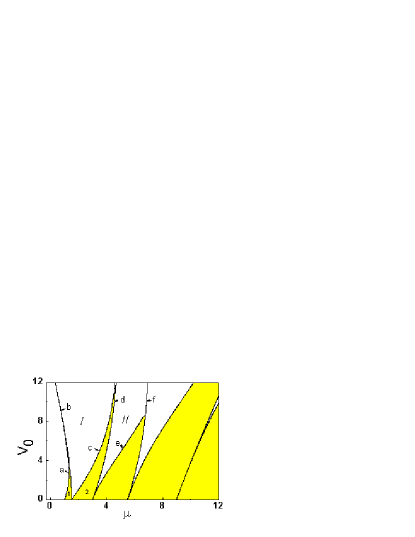
Figure 1: (Color online). Bloch band of BEC in an optical lattice in the linear regime is functions of the optical depth $V_{0}$ and the chemical potential $\mu$. The shaded areas denote the energy bands. The regions 1 and 2 represent the first and second energy band respectively. The areas $I$ and $II$ represent the lowest two band gaps in the spectrum. Band edges (solid line) a, $b,c,d,e,f,\cdots$ correspond to the eigenvalues and eigenstates $P^{c}_{0}(ce_{0}),P^{s}_{1}(se_{1}),P^{c}_{1}(ce_{1}),P^{s}_{2}(se_{2}),P^{c}_{2}(ce_{2}),P^{s}_{3}(se_{3}),\cdots$ of Mathieu’s equation, respectively.

We next consider the case of $Q^{\prime}\neq 0$, and discuss the stability problem of soliton formation. Utilizing Eqs. (8)-(10), we obtain

$$\omega^{2}=(\frac{1}{2u_{0}}\frac{\partial^{2}u_{0}}{\partial z^{2}}+\frac{1}{2}k^{2}+2Q^{\prime}u^{2}_{0})(\frac{ik}{u_{0}}\frac{\partial u_{0}}{\partial z}+\frac{1}{2}k^{2}).$$ (12)

Setting $\omega=\omega_{r}+i\omega_{i}$ (where the subscripts denote the real and imaginary parts) 35 , one gets that $\omega^{2}_{r}=(\gamma/4)\sqrt{k^{4}+(4k^{2}/u^{2}_{0})(\frac{\partial u_{0}}{\partial z})^{2}}+(k^{2}\gamma/4)$ and $\omega^{2}_{i}=(\gamma/4)\sqrt{k^{4}+(4k^{2}/u^{2}_{0})(\frac{\partial u_{0}}{\partial z})^{2}}-(k^{2}\gamma/4)$, where $\gamma=[1/(2u_{0})]\frac{\partial^{2}u_{0}}{\partial z^{2}}+k^{2}/2+2Q^{\prime}u^{2}_{0}$. If the imaginary part of quasi-particle frequency is a nonzero value, the corresponding Bloch wave exhibits exponential growth and hence the state $\psi$ is dynamical instability 22 . If the frequency of the associated quasi-particle spectrum is real, the soliton would be stable. From the expression of the imaginary part of the frequency, one can see the dependence of the instability growth rate $\omega_{i}$ on $k$ and $\frac{1}{u_{0}}\frac{\partial u_{0}}{\partial z}$. On the one hand, when $k=0$, one finds $\omega=0$, which is an inessential solution. On the other hand, it is impossible for $\frac{1}{u_{0}}\frac{\partial u_{0}}{\partial z}$ being equal to zero because $u_{0}$ is the Bloch wave in the energy bands or band gaps. If $\frac{1}{u_{0}}\frac{\partial u_{0}}{\partial z}$ is a purely imaginary number (also obtained from Eq. (12)), the wave function $\psi$ possesses dynamical stability. We therefore conclude that the stable condition of soliton formation is $u_{0}=\exp(i\beta z)$ where $\beta$ is an arbitrary real constant. Because the Bloch wave in the $nth$ energy band is the linear superposition of the Mathieu’s functions $ce_{n-1}$ and $se_{n}$, it always not satisfies the stable condition. Only if Bloch wave in the $nth$ band gap has the form of $u_{0}=\beta ce_{n}+\beta ise_{n}$, soliton possesses dynamical stability. Thus the linear dispersion relation of the $nth$ band gap is

$$\omega^{2}=(\frac{k^{2}}{2}-\frac{kn\pi}{D})(\frac{k^{2}}{2}-\frac{n^{2}\pi^{2}}{2D^{2}}+2Q^{\prime}u^{2}_{0}).$$ (13)

Under long-wave approximation, the sound speed is

$$V_{g}=\lim_{k\longrightarrow 0}\frac{\partial\omega}{\partial k}=\pm\sqrt{Q^{\prime}u^{2}_{0}-\frac{n^{2}}{4}(\frac{\pi}{D})^{2}},$$ (14)

where the positive (negative) sign represents the rightward (leftward) propagation of the wave packets. For the case of $D\longrightarrow\infty$, the external potential would be a harmonic potential [see Eq. (2)] and a corresponding sound speed is $V_{gh}=\sqrt{Q^{\prime}}u_{0}$ in our notation. This behavior is consistent with both the experimental 36 and theoretical results 29 . Obviously, the second term under the radical sign in Eq. (14) is arisen from the optical lattice potential. The sound speed is the largest in the first band gap and gradually decreases with $n$. Generally speaking, the value of $1/D$ in the experiments 23 ; 34 would be larger than that of $Q^{\prime}$. It implies that the linear dispersion relation and sound speed are dependent mainly on the lattice spacing.

IV IV. NONLINEAR BLOCH MODES

IV.1 A. The explicit expression of the wave function

To better understand the nonlinear dynamics of BEC in an optical lattice, we here develop a multiple scale method to derive an explicit expression of the wave function of the condensates in an optical lattice. By means of asymptotic expansion in nonlinear perturbation theory, we propose that the amplitude and phase can be expanded by multiple scale methods. In the case of that, mathematically, any parameter can be defined as a function of fast and slow variables, we propose each order parameter of the amplitude and phase can be written to a function of a fast and two slow variables. That is to say, the amplitude and phase of the wave function are sought for the forms of $A=u_{0}(z_{0},\xi,\tau)+\varepsilon[a^{(0)}(z_{0},\xi,\tau)+\varepsilon^{2}a^{(1)}(z_{0},\xi,\tau)+\cdots]$ and $\varphi=\varepsilon^{2}[\varphi^{(0)}(z_{0},\xi,\tau)+\varepsilon^{2}\varphi^{(1)}(z_{0},\xi,\tau)+\cdots]$, respectively, where the small parameter $\varepsilon$ represents the relative amplitude of extended states in BEC. Slow variables $\xi=\varepsilon(z-V_{g}t)$ and $\tau=\varepsilon^{3}t$ characterize the slow variation of soliton dynamics. Fast variable $z_{0}=z$ denotes the propagation direction of the lattice wave packets. $V_{g}$ is a group velocity. By substituting them into Eqs. (6) and (7), and then separating them in terms of $\varepsilon$, Eq. (6) can be written as

$$V_{g}\frac{\partial u_{0}}{\partial\xi}=0,$$ (15)

$$V_{g}\frac{\partial a^{(0)}}{\partial\xi}=\frac{\partial u_{0}}{\partial z_{0}}\frac{\partial\varphi^{(0)}}{\partial z_{0}}+\frac{1}{2}u_{0}\frac{\partial^{2}\varphi^{(0)}}{\partial z^{2}_{0}},$$ (16)

$$\frac{\partial u_{0}}{\partial z_{0}}\frac{\partial\varphi^{(0)}}{\partial\xi}+\frac{\partial u_{0}}{\partial\xi}\frac{\partial\varphi^{(0)}}{\partial z_{0}}+\frac{\partial a^{(0)}}{\partial z_{0}}\frac{\partial\varphi^{(0)}}{\partial z_{0}}=-\frac{\partial u_{0}}{\partial\tau},$$ (17)

$$V_{g}\frac{\partial a^{(1)}}{\partial\xi} =\frac{\partial a^{(0)}}{\partial\tau}+\frac{\partial a^{(0)}}{\partial\xi}\frac{\partial\varphi^{(0)}}{\partial z_{0}}+\frac{1}{2}u_{0}\frac{\partial^{2}\varphi^{(0)}}{\partial\xi^{2}}$$ (18)

$$+\frac{1}{2}u_{0}\frac{\partial^{2}\varphi^{(1)}}{\partial z^{2}_{0}}+a^{(0)}\frac{\partial^{2}\varphi^{(0)}}{\partial z_{0}\partial\xi}+\frac{\partial u_{0}}{\partial z_{0}}\frac{\partial\varphi^{(1)}}{\partial z_{0}}$$

$$+\frac{\partial u_{0}}{\partial\xi}\frac{\partial\varphi^{(0)}}{\partial\xi}+\frac{\partial a^{(0)}}{\partial z_{0}}\frac{\partial\varphi^{(0)}}{\partial\xi}.$$

Equation (7) becomes

$$-\frac{1}{2}\frac{\partial^{2}u_{0}}{\partial z^{2}_{0}}-(\mu-1)u_{0}+V_{0}\sin^{2}(\frac{\pi z_{0}}{D})u_{0}+Q^{\prime}u^{3}_{0}=0,$$ (19)

$$-\frac{1}{2}\frac{\partial^{2}a^{(0)}}{\partial z^{2}_{0}} - (\mu-1)a^{(0)}+V_{0}\sin^{2}(\frac{\pi z_{0}}{D})a^{(0)}$$ (20)

$$+3Q^{\prime}u^{2}_{0}a^{(0)}=\frac{\partial^{2}u_{0}}{\partial z_{0}\partial\xi},$$

$$-\frac{\partial^{2}a^{(0)}}{\partial z_{0}\partial\xi}+3Q^{\prime}u_{0}(a^{(0)})^{2}=\frac{1}{2}\frac{\partial^{2}u_{0}}{\partial\xi^{2}},$$ (21)

$$-\frac{1}{2}\frac{\partial^{2}a^{(1)}}{\partial z^{2}_{0}} - (\mu-1)a^{(1)}+V_{0}\sin^{2}(\frac{\pi z_{0}}{D})a^{(1)}$$ (22)

$$+3Q^{\prime}u^{2}_{0}a^{(1)}=\frac{1}{2}\frac{\partial^{2}a^{(0)}}{\partial\xi^{2}},$$

$$\frac{\partial^{2}a^{(1)}}{\partial z_{0}\partial\xi} - 6Q^{\prime}u_{0}a^{(0)}a^{(1)}=\frac{1}{2}u_{0}(\frac{\partial\varphi^{(0)}}{\partial z_{0}})^{2}$$ (23)

$$-V_{g}a^{(0)}\frac{\partial\varphi^{(0)}}{\partial\xi}.$$

From Eq. (15), one can see that $u_{0}$ is independent on $\xi$. Due to the fast and slow varies possess different physical connotation, so it is reasonable that these order parameters are written to arithmetic multiply of function of the fast and slow variables. We may set $u_{0}(z_{0},\tau)=u_{01}(z_{0})u_{03}(\tau)$. Similarly, $a^{(i)}$ and $\varphi^{(i)}$ are the forms of $a^{(i)}(z_{0},\xi,\tau)=a_{i1}(z_{0})a_{i2}(\xi)a_{i3}(\tau)$ and $\varphi^{(i)}(z_{0},\xi,\tau)=\varphi_{i1}(z_{0})\varphi_{i2}(\xi)\varphi_{i3}(\tau)$, respectively, where $i=0,1,2\cdots$. Note that the form of Eq. (19) is the same as that of Eq. (9). In view of the fact that BEC in the experiments are dilute and weakly interacting: $n|a_{s}|^{3}\ll 1$, where $n$ is the average density of the condensate, so Eq. (19) can also be transformed into Mathieu’s equation under the consideration of weak nonlinearity. The solutions of Mathieu’s equation have been discussed in section III. By comparing Eq. (19) with Eq. (20), one finds $a^{(0)}=0$. From Eq. (16), we obtain $u_{0}=(\frac{\partial\varphi^{(0)}}{\partial z_{0}})^{-(1/2)}$. So, Eq. (17) becomes

$$-\frac{\frac{\partial\varphi_{03}}{\partial\tau}}{\varphi^{2}_{03}}=\frac{\frac{\partial^{2}\varphi_{01}}{\partial z^{2}_{0}}\varphi_{01}\frac{\partial\varphi_{02}}{\partial\xi}}{\frac{\partial\varphi_{01}}{\partial z_{0}}}.$$ (24)

The left hand side of Eq. (24) is the differentiation of $\varphi_{03}$ with respect to $\tau$, while the right hand side of Eq. (24) is differentiation of $\varphi_{01}$ ($\varphi_{02}$) with respect to $z_{0}$ ($\xi$). Obviously, both sides of the equation must be equal to a constant $\lambda$, i.e., $\varphi_{03}=1/(\lambda\tau)$, and $\varphi_{02}=-(1/2)\lambda u_{01}\xi[\frac{\partial u_{01}}{\partial z_{0}}\int\frac{dz_{0}}{[u_{01}(z_{0})]^{2}}]^{-1}$. So, $\varphi^{(0)}=-[u_{01}\xi/(2\tau)][\frac{\partial u_{01}}{\partial z_{0}}]^{-1}$. Correspondingly, we get

$$\frac{\partial u_{03}(\tau)}{\partial\tau}=\frac{u_{03}(\tau)}{2\tau}.$$ (25)

Similarly, from Eqs. (18), (22) and (23), we have

$$a^{(1)}=\frac{u_{0}\xi^{3}}{24\tau^{2}[\frac{\partial^{2}u_{0}}{\partial z^{2}_{0}}+4Q^{\prime}u^{3}_{0}]}\frac{\partial}{\partial z_{0}}\{u_{0}[1-u_{0}\frac{\partial^{2}u_{0}}{\partial z^{2}_{0}}(\frac{\partial u_{0}}{\partial z_{0}})^{-2}]^{2}\}.\\ ~{}$$

Under the transformations $z_{0}=z$, $\xi=\varepsilon(z-V_{g}t)$, and $\tau=\varepsilon^{3}t$, the perturbation parameters can be written as $u_{0}(z,t)=u_{01}(z)\sqrt{t}$, $\varepsilon^{2}\varphi^{(0)}=-[(z-V_{g}t)u_{0}/(2t)][\frac{\partial u_{0}}{\partial z}]^{-1}$, and $\varepsilon^{3}a^{(1)}=\{u_{0}(z-V_{g}t)^{3}/[24t^{2}(\frac{\partial^{2}u_{0}}{\partial z^{2}}+4Q^{\prime}u^{3}_{0})]\}\frac{\partial}{\partial z}\{u_{0}[1-u_{0}\frac{\partial^{2}u_{0}}{\partial z^{2}}(\frac{\partial u_{0}}{\partial z})^{-2}]^{2}\}$, where $u_{01}(z)$ is the nonlinear Bloch wave of BEC in an optical lattice. Finally, the solution of the dimensionless GP equation (3) is given by

$$\psi(r,z,t) = \sqrt{\frac{1}{\pi}}\exp(-\frac{r^{2}}{2})\{u_{01}+\frac{u_{01}(z-V_{g}t)^{3}}{24t^{2}[\frac{\partial^{2}u_{01}}{\partial z^{2}}+4tQ^{\prime}u^{3}_{01}]}$$ (26)

$$\times\frac{\partial}{\partial z}\{u_{01}[1-u_{01}\frac{\partial^{2}u_{01}}{\partial z^{2}}(\frac{\partial u_{01}}{\partial z})^{-2}]^{2}\}\}$$

$$\times\exp[-i\mu t-i\frac{(z-V_{g}t)u_{01}}{2t}(\frac{\partial u_{01}}{\partial z})^{-1}].$$

where the Bloch waves $u_{01}$ and group velocity $V_{g}$ can be given in Sec. III. $\mu$ is the chemical potential. Equation (26) is just an explicit expression of the wave function for 1D BEC trapped in an optical lattice.

As is discussed in Sec. III, the Bloch wave in the $nth$ energy band is the linear superposition of the Mathieu’s functions $ce_{n-1}$ and $se_{n}$, which is always not satisfy the stable condition of soliton formation. Therefore, the condensate in the energy band region can not generate soliton, only the condensates in the band gaps may be occur the soliton. In the following we discuss soliton dynamical stabilities of the condensates in the band gaps. The stability of soliton in nonlinear systems is an important issue, since only dynamically stable modes are likely to be generated and observed in experiments.

IV.2 B. Soliton properties in the band gaps

To link our analytical results to real experiments, we estimate the values of the dimensionless parameters in Eq. (26) according to actual physical quantities. We consider a cigar-shaped ⁸⁷Rb condensate (atomic mass $1.4\times 10^{-25}$ $kg$ and the scattering length $5.3$ $nm$) containing $N=900$ atoms in a trap with $\omega_{z}=2\pi\times 0.5$ Hz and $\omega_{\bot}=2\pi\times 85$ Hz (The data are from the experiment 23 ). The parameter $\Omega\approx 0.006\ll 1$ in Eq. (3). It implies that the condensate may be regarded as a quasi-1D optical lattice in the direction of a weak confinement. Hereafter the radial radius is determined by $r=0.01$. Based on that 1D optical lattice is created from one pair of counter-propagating laser beams in real experiments, the lattice depth and the lattice spacing depend on the peak intensity and the angle of the two identical counter-propagating laser beams, respectively. For the wavelength $\lambda_{L}=783$ $nm$, used in Ref. 23 , this angle between counter-propagating laser beams would be equal to $2.3^{o}$. The periodic potential is $V=E_{0}\sin^{2}(\pi Z/d)$ where $E_{0}=0.70$ $E_{rec}$ and $d=\lambda_{L}/2$ are the lattice depth and periodicity, respectively. Accordingly, the time and space units correspond to $0.2$ $ms$ and $3$ $\mu m$, respectively. These units remain valid for other values of $N$, as one may vary $V_{0}$ accordingly; in this case, other quantities, such as $D$, also change. Based on these proposed, we obtain the dimensionless parameters $D\approx 0.33$, $Q^{\prime}\approx 9\times 10^{-3}$ and $V_{0}\approx 7.9$.

As is discussed above, the nonlinear Bloch waves in the $nth$ band gap can be given by the linear superposition of $ce_{n}$ and $se_{n}$ under the case of weak nonlinearity. On the basis of the fact that the coefficients of periodic Mathieu’s functions depend on eigenvalue $q$ 33 (i.e., $V_{0}$ in our notation), we presuppose that the Mahtieu’s functions are $ce_{1}=\sum\limits^{1000}_{k=0}V_{0}\cos(k\eta)$ and $se_{1}=\sum\limits^{1000}_{k=0}V_{0}\sin(k\eta)$ in the following calculation.

First, we choose a linear superposition form of $u_{01}(z)=ce_{1}+se_{1}$ as the nonlinear Bloch wave in the first band gap. The time-evolution of the density distribution of the condensates in this case is plotted in Fig. 2. We see that the peak of wave packets decreases exponentially with time and eventually vanishes. Thus the state is always unstable and be called sub-fundamental soliton in Ref. 37 . Such a soliton with a very small initial total number of atoms loses a part of atoms with time going on, so it is unstable (refer to Ref. 37 ).

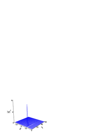
Figure 2: (Color online). The space-time evolution of the density of the condensates in the first band gap. The Bloch wave is chosen as $u_{01}(z)=ce_{1}+se_{1}$. The parameters used are the lattice depth $V_{0}=7.9$, interatomic interaction strength $Q^{\prime}=9\times 10^{-3}$, the lattice spacing $D=0.33$, the radial radius $r=0.01$, and the chemical potential $\mu=1.12$. All parameters are in dimensionless units.

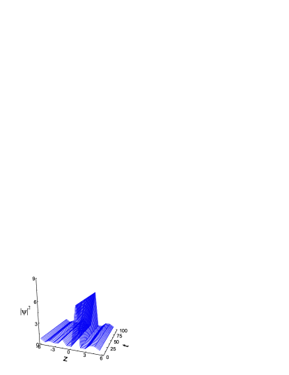
Figure 3: (Color online). The space-time evolution of the density of the condensate with $12.6$ dimensionless lengths (about 38 lattice sites), which corresponds to about $38\mu m$ in real space. The Bloch wave is chosen as $u_{01}(z)=ce_{1}+ise_{1}$. Other parameters used are the same as Fig. 2

Secondly, we choose $u_{01}(z)=ce_{1}+ise_{1}$, which satisfies the stable condition of soliton formation, as the nonlinear Bloch wave in the first band gap. Figure 3 shows the space-time evolution of the density the condensates in first band gap. A strong peak appears in the condensate with a dimensionless lengths of 12.6 (about $38$ lattice sites), and maintains its shape and magnitude. It implies the existence of a bright gap soliton. As the time going on, the bright gap soliton is pinned in the optical lattice without both attenuation and change in shape. This behavior indicates that it is a spatially localized bright gap soliton, which is arisen from the interplay between the tunneling of periodical potential and nonlinear interaction of the system. Moreover, the width of the peak in the $z-t$ plane is found to be a dimensionless length with 2.0, i.e., $\approx 6$ $\mu m$ in real space. The value is in good agreement with that of the experiment observed by Eiermann et al. 23 . The agreement illustrates that our method can describe the dynamics of BEC trapped in an optical lattice very well. The type of bright gap solitons are called fundamental solitons in Ref. 37 . Similar phenomena can also be obtained inside the other band gap.

From the results discussed above, the solitons residing in the band gaps are the fundamental or sub-fundamental solitons depending on their position in the band gap whether the stable condition of soliton formation can be satisfied or not.

In real experiment, the 1D optical lattice is created from one pair of counter-propagating laser beams, and the lattice depth depends on the peak intensity of the two identical counter-propagating laser beams. That is to say, the lattice depth can be adjusted by varying the intensity of the counter-propagating laser beams. We here depict how the lattice depth influences the fundamental soliton in Fig. 4 (with all the rest of the system parameters fixed). From solid line ($V_{0}=7.9$) and dashed line ($V_{0}=10$), one sees the amplitude of the fundamental soliton increasing with the increasing of the lattice depth. Due to both wave packets containing the same total number of atoms but the bosons in deeper well are captured more tightly, the tunneling probability varies smaller 18 ; niu . To balance the same nonlinear effect of the system, the tunneling rate of bosons in deeper well becomes much larger to achieve the same dispersion effect, which results in the amplitude of the fundamental soliton increasing. Therefore, the amplitude of the localized gap soliton increases with the increasing the intensity of the counter-propagating lasers beams in the experiments.

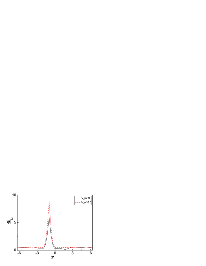
Figure 4: (Color online). The distribution of the density of the condensates with different lattice depth at $t=1$, where the dimensional parameter $V_{0}=7.9$ corresponds to the lattice depth in the experiment 23 . Other parameters used are the same as Fig. 2.

Subsequently, we observe the soliton characteristics in a longer condensate. Our numerical calculations are performed for the condensate cloud in the ground state extending over 35 dimensionless lengths (about 106 lattice sites), which corresponds to $105$ $\mu m$ in real space. The condensate cloud contains about $2.5\times 10^{3}$ atoms under the consideration that the atomic density keeps unchanged. Fig. 5 shows the space-time evolution of the density of the condensates in this case. It is shown that there exhibits a localized gap soliton train consisting of several fundamental solitons in the condensate. Similarly to the property of a single fundamental soliton, the solitonlike wave packets in the train are immobile (i.e., have zero group velocity). In reality, the condensate is loaded into an optical lattice from a crossed optical dipole trap 23 , which results in an initial state of a finite extent. A BEC wave packet centered around a particular quasimomentum in a given band is created by ramping up of a static lattice with subsequent linear acceleration to a given velocity 23 . In order to observe a localized gap soliton train, we may propose experimental protocols according to the experimental observation of a single fundamental soliton 23 . First, the atoms are initially precooled in a magnetic time-orbiting potential trap using the standard technique of forced evaporation leading to a phase space density of $\sim 0.03$. Subsequently, the atomic ensemble is adiabatically transferred into a crossed light beam dipole trap, where further forced evaporation is achieved by lowering the light intensity in the trapping light beams. With this approach, one can generate pure condensates with typically $9\times 10^{4}$ atoms. By further lowering the light intensity, one can reliably produce coherent wave packets of $9000$ atoms. For this atom number no gap solitons have been observed. Therefore, one removes atoms by Bragg scattering. This method splits the condensate coherently leaving an initial wave packet with $2.5\times 10^{3}$ atoms at rest. Then, the wave packet centered on a particular position in a given band gap (which satisfies the stable condition of soliton formation) is created by switching off one dipole trap beam from a crossed optical dipole trap, releasing the atomic ensemble into 1D horizontal waveguide with transverse and longitudinal trapping frequencies $\omega_{\bot}=2\pi\times 85$ $Hz$, and $\omega_{\|}=2\pi\times 0.5$ $Hz$, and then accelerating the periodic potential to the recoil velocity $v_{r}=h/m\lambda$. This is done by introducing an increasing frequency difference between the two laser beams, creating the optical lattice. The acceleration is adiabatic, which results in an initial state of an about $105$ $\mu m$ extent. In view of the fact that the tunneling rate of about 900 atoms extending the length of $38$ $\mu m$ (in our above simulation) can balance its nonlinear energy, such a system generates a fundamental soliton. With both the length of condensate and the total number of atoms increase, the wave packet exhibits violent dynamics. During this evolution the wave packet containing $2.5\times 10^{3}$ atoms is separated from the surrounding atomic cloud into several BEC wave packets, so the periodic structure of a train of the localized wave packets emerges. Such a structure represents a train consisting of several fundamental solitons, which is supported by the combined action of the repulsive nonlinearity and anomalous diffraction caused by intersite tunneling in the band gaps 15 ; 17 ; 38 .

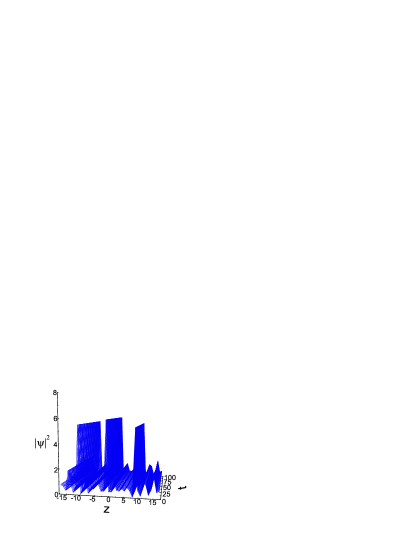
Figure 5: (Color online). The space-time evolution of the density of the condensate with 35 dimensionless lengths (about 106 lattice sites), which corresponds to about $105\mu m$ in real space. Other parameters used are the same as Fig. 2.

Finally, we study how the lattice spacing influences the fundamental soliton or soliton trains as shown in Fig. 6. In practice the variation of lattice spacing is easy to control by adjusting the angle between two counter-propagating laser beams. From solid line ($D=0.33$) and dashed line ($D=0.99$), we find that when lattice spacing occurs a slight difference, the pinning position and the amplitude of each fundamental soliton have a little change keeping the distance between adjacent solitons unvaried. It illuminates that the condensate cloud is separated into three wave packets for both $D=0.33$ and $D=0.99$. When the lattice spacing $D$ varies from 0.33 to 0.99, the condensate from 91 decreases to 30 wells. Owing to the center position of each wave packet floating, the pinning position of the fundamental soliton are set to move. And each BEC wave packet still forms a localized gap soliton, which comes from the balance between the nonlinearity and atom dispersion caused by intersite tunneling. However, when the lattice spacing $D$ varies from $0.33$ to $0.99$, the number of atoms in a well increases from $28$ to $83$. For the same length condensate, the tunneling between adjacent well varies easier with the increasing of the atomic number confined in a well. To balance the same nonlinear energy of the system, bosons gathering around several wells vary easier, which results in the amplitude of each localized soliton having a increasing trend. When lattice spacing varies much larger [see dotted line $D=16.5$ in Fig. 6], one find that there appears only a fundamental soliton in the entire condensate with about 30 dimensionless lengths. This mainly reason is that the condensate in this case only contains about 2 wells. The tunneling of bosons in adjacent lattice achieves the dispersion effect to balance the nonlinear energy of the system, so there exhibits only a fundamental soliton in this case.

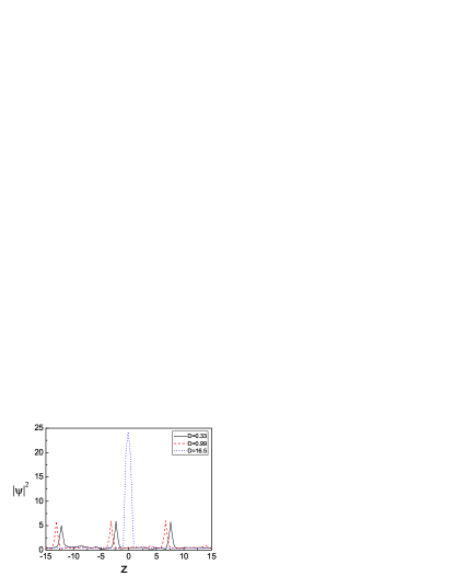
Figure 6: (Color online). The distribution of the density of the condensates with different lattice spacing $D$ at $t=1$, where the dimensional parameter $D=0.33$ corresponds to the lattice spacing in the experiment 23 . Other parameters used are the same as Fig. 2.

From the results discussed above, we can conclude that the condensate generating a single fundamental soliton or a localized gap soliton train consisting of several fundamental solitons can be controlled by adjusting the length of condensate or (and) the lattice spacing. Our theoretical results reported here is important in understanding the fundamental soliton physics of BEC in the future.

V V. CONCLUSION

In summary, we develop the multiple scale method to study the linear and nonlinear solitary excitations for 1D BEC confined in an optical lattice. After averaging over the transverse variable, a hydrodynamical model of the amplitude and phase is derived. In the linear case, the Bloch wave in the $nth$ energy band is the linear superposition of the Mathieu’s functions $ce_{n-1}$ and $se_{n}$, and the Bloch wave in the $nth$ band gap is the linear superposition of $ce_{n}$ and $se_{n}$. In addition, we find that the stable condition of soliton formation is that the Bloch wave $u_{0}$ in $nth$ band gap satisfies $u_{0}=\beta ce_{n}+i\beta se_{n}$. Under this stable condition, a novel linear dispersion relation and sound speed are derived. It is found that the linear dispersion relation and sound speed depend mainly on the lattice spacing.

For the nonlinear case, we derive a solution of the wave function of the condensates with weakly inter-atomic interaction, and discuss its stability for condensate ${}^{87}Rb$ in band gaps. It shows that there are two types of gap solitons in the band gaps. One is fundamental soliton, which is always stable and pins a fixed position; the other is subfundamental soliton which is always unstable and decays gradually due to losing a part of its atoms. Only when the Bloch wave in the band gaps satisfies the stable condition, the condensates exhibit the fundamental solitons, otherwise there appears the sub-fundamental solitons. Furthermore, the pinning position and the amplitude of the fundamental solitons in the lattice can be controlled by varying the lattice depth and spacing. We also propose an experimental protocol to observe a localized gap soliton train consisting of several fundamental solitons for BEC trapped in an optical lattice in future experiment.

VI ACKNOWLEDGMENTS

This work is supported by NSF of China under Grant 90406017, 60525417, 10740420252, 10674070, 10674113, the NKBRSF of China under Grant 2005CB724508, 2006CB921400, Jiangsu Provincial Postdoctoral Science Foundation under Grant 0601043B, and Hunan provincial NSF of China under Grant 06JJ50006.

References

- (1) M. Barrett, J. Sauer, and M. S. Chapman, Phys. Rev. Lett. 87, 010404 (2001).
- (2) C. Orzel, A. K. Tuchman, M. L. Fensclau, M. Yasuda, and M. A. Kasevich, Science 291, 2386 (2001).
- (3) F. S. Cataliotti, S. Burger, C. Fort, P. Maddaloni, F. Minardi, A. Trombettoni, A. Smerzi, and M. Inguscio, Science 293, 843 (2001).
- (4) M. Greiner, O. Mandel, T. Esslinger, T. W. Hansch, and I. Bloch, Nature 415, 39 (2002).
- (5) A. S. Desyatnikov, E. A. Ostrovskaya, Y. S. Kivshar, and C. Denz1, Phys. Rev. Lett. 91, 153902 (2003); G. P. Berman, F. Borgonovi, F.M. Izrailev, and A. Smerzi, Phys. Rev. Lett. 92, 030404 (2004); J. Yang, I. Makasyuk, P. G. Kevrekidis, H. Martin, B. A. Malomed, D. J. Frantzeskakis, and Z. G. Chen, Phys. Rev. Lett. 94, 113902 (2005).
- (6) B. B. Baizakov, B. A. Malomed, and M. Salerno, Phys. Rev. E 74, 066615 (2006); H. Sakaguchi and B. A. Malomed, Phys. Rev. E 72, 046610 (2005); B. Baizakov, G. Filatrella, B. Malomed, and M. Salerno, Phys. Rev. E 71, 036619 (2005).
- (7) K. Staliunas, R. Herrero, and G. J. de Valc rcel, Phys. Rev. E 73, 065603 (2006); G. X. Huang, L. Deng, and C. Hang, Phys. Rev. E 72, 036621 (2005); D. E. Pelinovsky, D. J. Frantzeskakis, and P. G. Kevrekidis, Phys. Rev. E 72, 016615 (2005).
- (8) E. Kengne and W. M. Liu, Phys. Rev. E 73, 026603 (2006); L. Li, B. A. Malomed, D. Mihalache, and W. M. Liu, Phys. Rev. E 73, 066610 (2006); V. A. Brazhnyi and V. V. Konotop, Phys. Rev. E 72, 026616 (2005).
- (9) G. Theocharis, D. J. Frantzeskakis, R. C. Gonz lez, P. G. Kevrekidis, and B. A. Malomed, Phys. Rev. E 71, 017602 (2005); D. E. Pelinovsky, A. A. Sukhorukov, and Y. S. Kivshar, Phys. Rev. E 70, 036618 (2004); B. A. Malomed, T. Mayteevarunyoo, E. A. Ostrovskaya, and Y. S. Kivshar, Phys. Rev. E 71, 056616 (2005).
- (10) E. P. Fitrakis, P. G. Kevrekidis, H. Susanto, and D. J. Frantzeskakis, Phys. Rev. E 75, 066608 (2007); D. L. Machacek, E. A. Foreman, Q. E. Hoq, P. G. Kevrekidis, A. Saxena, D. J. Frantzeskakis, and A. R. Bishop, Phys. Rev. E 74, 036602 (2006).
- (11) Z. X. Liang, Z. D. Zhang, and W. M. Liu, Phys. Rev. Lett. 94, 050402 (2005); A. C. Ji, X. C. Xie, and W. M. Liu, Phys. Rev. Lett. 99, 183602 (2007).
- (12) A. Trombettoni and A. Smerzi, Phys. Rev. Lett. 86, 2353 (2001); A. Smerzi and A. Trombettoni, Phys. Rev. A 68, 023613 (2003).
- (13) F. K. Abdullaev, B. B. Baizakov, S. A. Darmanyan, V. V. Konotop, and M. Salerno, Phys. Rev. A 64, 043606 (2001).
- (14) O. Zobay, S. Pötting, P. Meystre, and E. M. Wright, Phys. Rev. A 59, 643 (1999).
- (15) G. L. Alfimov, P. G. Kevrekidis, V. V. Konotop, and M. Salerno, Phys. Rev. E 66, 046608 (2002).
- (16) H. Pu, L. O. Baksmaty, W. Zhang, N. P. Bigelow, and P. Meystre, Phys. Rev. A 67, 043605 (2003).
- (17) N. K. Efremidis and D. N. Christodoulides, Phys. Rev. A 67, 063608 (2003).
- (18) V. V. Konotop and M. Salerno, Phys. Rev. A 65, 021602(R) (2002).
- (19) O. Morsch and M. Oberthaler, Rev. Mod. Phys. 78, 179 (2006).
- (20) K. M. HilligOe, M. K. Oberthaler, and K. P. Marzlin, Phys. Rev. A 66, 063605 (2002); V. Ahufinger, A. Sanpera, P. Pedri, L. Santos, and M. Lewenstein, Phys. Rev. A 69, 053604 (2004).
- (21) S. Pötting, M. Cramer, and P. Meystre, Phys. Rev. A 64, 063613 (2001); H. A. Cruz, V. A. Brazhnyi, V. V. Konotop, G. L. Alfimov, and M. Salerno, Phys. Rev. A 76, 013603 (2007).
- (22) P. J. Y. Louis, E. A. Ostrovskaya, C. M. Savage, and Y. S. Kivshar, Phys. Rev. A 67, 013602 (2003).
- (23) B. Eiermann, T. Anker, M. Albiez, M. Taglieber, P. Treutlein, K. P. Marzlin, and M. K. Oberthaler, Phys. Rev. Lett. 92, 230401 (2004).
- (24) T. Mayteevarunyoo and B. A. Malomed, Phys. Rev. A 74, 033616 (2006).
- (25) E. A. Ostrovskaya and Y. S. Kivshar, Phys. Rev. Lett. 90, 160407 (2003).
- (26) M. Matuszewski, W. Kr likowski, M. Trippenbach, and Y. S. Kivshar, Phys. Rev. A 73, 063621 (2006).
- (27) P. G. Kevrekidis, D. J. Frantzeskakis, R. C. Gonz lez, B. A. Malomed, G. Herring, and A. R. Bishop, Phys. Rev. A 71, 023614 (2005).
- (28) C. Menotti, M. Krämer, A. Smerzi, L. Pitaevskii, and S. Stringari, Phys. Rev. A 70, 023609 (2004).
- (29) T. Busch and J. R. Anglin, Phys. Rev. Lett. 84, 2298 (2000).
- (30) G. X. Huang, M. G. Velarde, and V. A. Makarov, Phys. Rev. A 64, 013617 (2001); G. X. Huang, J. Szeftel, and S. H. Zhu, Phys. Rev. A 65, 053605 (2002).
- (31) A. E. Muryshev, H. B. vanLindenvandenHeuvell, and G. V. Shlayapnikov, Phys. Rev. A 60, 2665(R) (1999).
- (32) D. W. Jordan and P. Smith, Nonlinear Ordinary Differential Equations (Clarendon Press, Oxford, 1977).
- (33) I. S. Gradshteyn and I. M. Rhyzhik, Table of Integrals, Series, and Products, 4th ed. (academic, New York, 1980), P. 991, Sec. 8.60.
- (34) M. Cristiani, O. Morsch, J. H. M ller, D. Ciampini, and E. Arimondo, Phys. Rev. A 65, 063612 (2002); O. Morsch, M. Cristiani, J. H. M ller, D. Ciampini, and E. Arimondo, Phys. Rev. A 66, 021601(R) (2002).
- (35) P. G. Kevrekidis, R. Carretero-Gonzalez, G. Theocharis, D. J. Frantzeskakis, and B. A. Malomed, Phys. Rev. A 68, 035602 (2003).
- (36) M. R. Andrews, D. M. Kurn, H. J. Miesner, D. S. Durfee, C. G. Townsend, S. Inouye, and W. Ketterle, Phys. Rev. Lett. 79, 553 (1997); 80, 2967 (1998).
- (37) Q. Niu, X. G. Zhao, G. A. Georgakis, and M. G. Raizen, Phys. Rev. Lett. 76, 4504 (1996); W. M. Liu, W. B. Fan, W. M. Zheng, J. Q. Liang, and S. T. Chui, Phys. Rev. Lett. 88, 170408 (2002).
- (38) B. J. Dabrowska, E. A. Ostrovskaya, and Y. S. Kivshar, Phys. Rev. A 73, 033603 (2006).