Abstract

In this talk, I shall first discuss the standard model Higgs mechanism and then highlight some of its deficiencies making a case for the need to go beyond the standard model (BSM). The BSM tour will be guided by symmetry arguments. I shall pick up four specific BSM scenarios, namely, supersymmetry, Little Higgs, Gauge-Higgs unification, and the Higgsless approach. The discussion will be confined mainly on their electroweak symmetry breaking aspects.

PACS Nos:  12.60.Jv, 11.10.Kk
Key Words:  Higgs, Supersymmetry, Extra Dimension

I Introduction

The understanding of electroweak symmetry breaking (EWSB) would be right at the top of the agenda when we would start analysing the LHC data [1, 2, 3, 4]. Both the CMS and the ATLAS detectors are poised to resolve this issue. The question is the following: whether the Higgs mechanism as depicted in the standard model (SM) is a complete description of EWSB consistent with all experimental data, or there is a more fundamental underlying dynamics that mimics a Higgs-like picture at the electroweak scale. On theoretical grounds, the latter seems to be the case. Then, in what form would that new physics beyond the standard model (BSM) manifest in the LHC data? We need to crack several codes before we can possibly unravel the most expensive secret challenging our imagination!

The SM reigns supreme at the electroweak scale and electroweak precision tests (EWPT), primarily at LEP, have put a lot of restraints on how a BSM scenario should be perceived. Non-abelian gauge theory has been established to a very good accuracy: (i) the $ZWW$ and $\gamma WW$ vertices have been measured to a per cent accuracy at LEP-2 implying that the SU(2) $\times$ U(1) gauge theory is unbroken at the vertices, (ii) accurate measurements of the $Z$ and $W$ masses have indicated that gauge symmetry is broken in masses, and the longitudinal polarizations of those gauge bosons, which are absent in the unbroken phase of the symmetry, should find their ancestry in the dynamics that portrays a Higgs-like picture. The $\rho$-parameter has been measured to a very good accuracy as being very close to unity - a feature that attests the doublet structure of the Higgs assumed in the SM. Any viable BSM scenario should be in accord to the above properties. In what follows, we first briefly review the SM Higgs mechanism and then take on supersymmetry, little Higgs, gauge-Higgs unification and the Higgsless models, keeping our discussions confined only to their EWSB aspects.

II The SM Higgs mechanism

There is a complex scalar doublet $\Phi\equiv\left(\phi_{1}+i\phi_{2},\phi_{3}+i\phi_{4}\right)^{T}$, and the potential is

$$V(\Phi)=-\mu^{2}\Phi^{\dagger}\Phi+\lambda(\Phi^{\dagger}\Phi)^{2}\,.$$ (1)

Spontaneous symmetry breaking (SSB) requires $\mu^{2}>0$, and the stability of the potential (that it is bounded from below) demands that $\lambda>0$. After SSB, an order parameter, called ‘vacuum expectation value (vev)’, is generated: $v=\sqrt{\mu^{2}/\lambda}$. The charged and neutral force particles, namely, the $W^{\pm}$ and $Z$ bosons, ‘swallow’ the $(\phi_{1},\phi_{2})$ and $\phi_{4}$ components of $\Phi$ to constitute their longitudinal polarizations, which yield $M_{W}=gv/2$ and $M_{Z}=(\sqrt{g^{2}+g^{\prime 2}})v/2$, where $g$ and $g^{\prime}$ are SU(2) and U(1) gauge couplings, respectively. The fermion masses are also controlled by $v$ and are given by $m_{f}=h_{f}v/\sqrt{2}$, where $h_{f}$ is the Yukawa coupling of the fermion $f$. The Higgs boson ($h$) arises from the quantum fluctuation of $\phi_{3}$ around the vev ($\phi_{3}=(v+h)/\sqrt{2}$), and $m_{h}=\sqrt{2\lambda}v$. The latest global electroweak fit gives $M_{Z}=91.1875\pm 0.0021$ GeV and $M_{W}=80.398\pm 0.025$ GeV.

II.1 Constraints on the Higgs mass

II.1.1 Electroweak fit

The Higgs mass enters electroweak fit through the $\Delta\rho$ and $S$ parameters. At the tree level, $\rho^{\rm SM}=1$. The quantum corrections show a logarithmic sensitivity to the Higgs mass:

$$\Delta\rho\simeq\frac{3G_{F}}{8\pi^{2}\sqrt{2}}\left[m_{t}^{2}-(M_{Z}^{2}-M_{W}^{2})\ln(\frac{m_{h}^{2}}{M_{Z}^{2}})\right],~{}~{}S\simeq\frac{1}{6\pi}\ln\left(\frac{m_{h}}{M_{Z}}\right).$$ (2)

There is a strong quadratic dependence on the top mass. At present, the CDF and D0 combined estimate is $m_{t}=172.6\pm 1.4$ GeV. This translates into an upper limit on the Higgs mass: $m_{h}<186$ GeV at 95% CL (imposing the direct search limit $m_{h}>114.4$ GeV in the fit, from non-observation of Higgs at LEP-2 in the Bjorken process $e^{+}e^{-}\to Zh$) [5]. Figs. 1a and 1b capture the details.

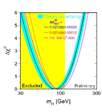
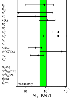
Figure 1: (a) Left panel: The blue-band plot showing the Higgs mass limits [5]. (b) The limits on the Higgs mass from different measurements. The central band corresponds to the ‘average’ [5].

II.1.2 Theoretical limits

Unitarity [6] places an upper bound on $m_{h}$ beyond which the theory becomes non-perturbative. Here, we shall call it a ‘tree level unitarity’ as we would require that the tree level contribution of the first partial wave in the expansion of different scattering amplitudes does not saturate unitarity (in other words, some probability should not exceed unity). The scattering amplitudes involving gauge bosons and Higgs can be decomposed into partial waves (using ‘equivalence theorem’) as

$$a_{J}(s)=\frac{1}{32\pi}\int d(\cos\theta)P_{J}(\cos\theta)M(s,\theta),$$ (3)

where $a_{J}$ is the $J$th partial wave, $P_{J}$ is the $J$th Legendre polynomial and $M(s,\theta)$ is the scattering matrix element. The most divergent scattering amplitude arises from $2W_{L}^{+}W_{L}^{-}+Z_{L}Z_{L}$ channel, leading to $a_{J=0}=-5m_{h}^{2}/64\pi v^{2}$. Satisfying the unitarity constraint, i.e. $|{\rm Re}~{}a_{J}|\leq 0.5$, yields $m_{h}<780$ GeV.

Besides, there are theoretical upper and lower limits on the Higgs mass arising from the twin requirements [7, 8]: (i) the running quartic coupling $\lambda(\mu)$ should not hit the Landau pole throughout the history of renormalization group (RG) evolution from the electroweak scale $v$ to some cutoff $\Lambda$, and (ii) $\lambda(\mu)$ should always stay positive, so that the scalar potential remains bounded from below. The bounds follow from the following RG evolution of the quartic coupling, given by ($t=\ln(\mu/v)$):

$$d\lambda/dt=(4\pi^{2})^{-1}3\left[\lambda^{2}+\lambda h_{t}^{2}-h_{t}^{4}-...\right]\,.$$ (4)

Recall, $m_{h}=\sqrt{\lambda(v)}v$, and that is how the Higgs mass enters into the game. The triviality argument of staying within the perturbative limit by maintaining $\lambda^{-1}(\mu)>0$ leads to an upper limit $m_{h}<170$ GeV for $\Lambda=10^{16}$ GeV. The vacuum stability argument, that $\lambda(\mu)>0$ bounds the potential from below, sets a lower limit $m_{h}>130$ GeV for $\Lambda=10^{16}$ GeV. The limits for other choices of the cutoff can be read off from Figs. 2a and 2b.

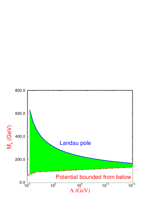
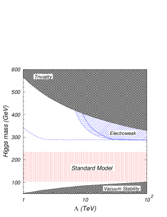
Figure 2: (a) Left panel: The triviality and vacuum stability limits [7]. (b) Right panel: The region upto $\Lambda=100$ TeV is zoomed. The hatched region ‘Electroweak’ is ruled out by precision data. Only the ‘Standard Model’ region is allowed at 95% CL [8].

II.2 Will the discovery of Higgs mark the end of the story?

Once we discover the Higgs, the SM spectrum is completed. But, will a completion be achieved in terms of our understanding of the universe through elementary particle interactions? We should remember that there are phenomena which cannot be explained by the SM: notably, the neutrino mass, the dark matter and the acceleration of the universe. Moreover, there is a conceptual loop-hole in the description of the scalar sector: the SM suffers from the gauge hierarchy problem. The quantum correction to the Higgs mass is quadratically sensitive to the cutoff,

$$\Delta m_{h}^{2}(f)=-\frac{h_{f}^{2}}{16\pi^{2}}2\Lambda^{2}~{}~{}~{}~{}~{},~{}~{}~{}~{}~{}\Delta m_{h}^{2}(S)=\frac{\lambda}{16\pi^{2}}\Lambda^{2}\,,$$ (5)

where $f$ and $S$ in brackets stand for fermionic and scalar loops. The cutoff dependence arises because no symmetry protects the Higgs mass. Recall that in QED the electron mass is protected by chiral symmetry, $\Delta m_{e}=m_{e}\frac{\alpha}{4\pi}\ln(\Lambda)$, so that $m_{e}\to 0$ gives an enhanced symmetry. In the electroweak theory after the SSB, as we can see from Eq. (5), there is no such enhanced symmetry when $m_{h}\to 0$. More precisely, the vev $v$ is not protected from large quantum corrections. Thus, while on one hand we demand the Higgs to weigh around a few hundred GeV, on the other hand the quantum correction pushes it up to the cutoff (e.g. the GUT scale). Even if we absorb the one-loop $\Lambda^{2}$ terms by a redifinition of $\mu^{2}$ or tuning $\lambda=2h_{f}^{2}$, when we go to two-loop the $\Lambda$-dependence again shows up with different coefficients, and thus we need to tune the parameters again. We have to repeat it order-by-order in perturbation theory, which makes the theory meaningless. This is what constitutes the gauge hierarchy problem. Since $v$ is not stable, not only the Higgs mass, the masses of the gauge bosons and fermions are not stable either.

Another bothering issue is the negative sign put by hand in front of $\mu^{2}$ in Eq. (1) to make SSB happen. We must have a dynamical understanding of this ad hoc ‘minus sign’.

Now we shall take a few examples of BSM scenarios and observe how in each case some underlying symmetry regulates the Higgs mass.

III Supersymmetry

III.1 Basics

Supersymmetry is a new space-time symmetry interchanging bosons and fermions, relating states of different spin [9, 10]. The Poincare group is extended by adding two anticommuting generators $Q$ and $\bar{Q}$, to the existing $p$ (linear momentum), $J$ (angular momentum) and $K$ (boost), such that $\{Q,\bar{Q}\}\sim p$. Since the new symmetry generators are spinors, not scalars, supersymmetry is not an internal symmetry. Recall, Dirac postulated a doubling of states by introducing an antiparticle to every particle in an attempt to reconcile Special Relativity with Quantum Mechanics. In Stern-Gerlach experiment, an atomic beam in an inhomogeneous magnetic field splits due to doubling of the number of electron states into spin-up and -down modes indicating a doubling with respect to angular momentum. So it is no surprise that $Q$ would cause a further splitting into particle and superparticle ($f\stackrel{{\scriptstyle Q}}{{\rightarrow}}f,\widetilde{f}$) [11]. Since $Q$ is spinorial, the superpartners differ from their SM partners in spin. The superpartners of fermions are scalars, called ‘sfermions’, and those of gauge bosons are fermions, called ‘gauginos’. Put together, a particle and its superpartner form a supermultiplet. The two irreducible supermultiplets which are used to construct the supersymmetric standard model are the ‘chiral’ and the ‘vector’ supermultiplets. The chiral supermultiplet contains a scalar (e.g. selectron) and a 2-component Majorana fermion (e.g. left-chiral electron). The vector supermultiplet contains a gauge field (e.g. photon) and a 2-component Majorana fermion (e.g. photino). Two points are worth noting: (i) there is an equal number of bosonic and fermionic degrees of freedom in a supermultiplet; (ii) since $p^{2}$ commutes with $Q$, the bosons and fermions in a supermultiplet are mass degenerate.

III.2 Motivation

III.2.1 Supersymmetry solves the gauge hierarchy problem

An attempt to solve the ‘gauge hierarchy problem’, i.e., why $M_{\rm Pl}\gg M_{W}$, or equivalently, $G_{N}\ll G_{F}$, is the main motivation behind the introduction of supersymmetry [12]. We recall from the previous section that quantum corrections to the Higgs mass from a bosonic loop and a fermionic loop have opposite signs. So if the couplings are identical and the boson is mass degenerate with the fermion, the net contribution would vanish! What can be a better candidate than supersymmetry to do this job? For every particle supersymmetry provides a mass degenerate partner differing by spin $1\over 2$. However, the cancellation is not exact because in real world supersymmetry is badly broken. But if the breaking occurs through ‘soft’ terms, i.e. in masses and not in couplings, the quadratic divergence still cancels. The residual divergence is mild, only logarithmically sensitive to the supersymmetry breaking scale.

III.2.2 Supersymmetry leads to unification of gauge couplings

This was a bonus [13]. Supersymmetry was introduced not with this in mind! In the SM, when the gauge couplings are extrapolated to high scale, with LEP measurements as input values, they do not meet at a single point. In supersymmetry, they do, at a scale $M_{\rm GUT}\sim 2\times 10^{16}$ GeV, provided the superparticles weigh around 1 TeV (see Fig. 3a).

III.2.3 Supersymmetry triggers EWSB

The mass-square of one of the Higgs, $m_{H_{u}}^{2}$, starting from a positive value in the ultraviolet becomes negative in the infrared triggering EWSB. As we remarked in the previous section that in the SM the negative sign in front of the scalar mass-square in the potential is completely ad hoc and put in by hand to ensure EWSB. In supersymmetry it is the heavy top quark that radiatively induces the sign flip (see Fig. 3b).

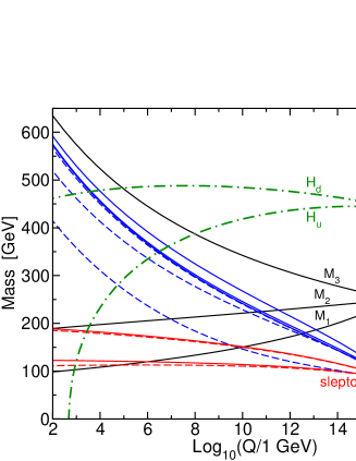
Figure 3: (a) Left panel: Gauge coupling unification in MSSM [13]. (b) Right panel: Negative $m_{H_{u}^{2}}$ in low energy triggers EWSB [10].

III.2.4 Supersymmetry provides a cold dark matter candidate

The present energy density (in units of critical density) of a thermal-relic particle ($\chi$) is theoretically calculated as $\Omega_{\chi}h^{2}\sim 0.1~{}{\rm pb}/\sigma$, where $\sigma$ is the thermal averaged non-relativistic cross section for $\chi\chi\to f\bar{f}$. The observed dark matter density is $\Omega_{\rm DM}h^{2}=0.114\pm 0.003$ [14]. Thus a weakly interacting particle with a $\sim 100$ GeV mass, which has a typical cross section of a pb, fits the bill! Interestingly, in the theoretical formula, the coefficient 0.1 was derived using cosmological parameters without any direct connection to the weak scale. This numerical coincidence deserves attention. Supersymmetry with conserved $R$-parity can provide such a dark matter candidate, a neutralino.

III.2.5 Supersymmetry provides a framework to turn on gravity

Local supersymmetry leads to supergravity. Thus gravity can be unified with all other interactions. All string models invariably include supersymmetry as an intergral part.

III.3 The parameters in a general supersymmetric model

In the minimal supersymmetric standard model (MSSM), where we do not assume any particular mediation mechanism for its breaking and do not impose any GUT conditions, the supersymmetry breaking soft parameters are not related to one another. Here, we will see how a general supersymmetric model can be parametrized [15].

First consider the superpotential, written in terms of the ‘chiral superfields’, as

$$W = \sum_{ij}\left(h_{e}^{ij}\hat{L}_{i}\hat{H}_{d}\hat{E}_{j}^{c}+h_{d}^{ij}\hat{Q}_{i}\hat{H}_{d}\hat{D}_{j}^{c}+h_{u}^{ij}\hat{Q}_{i}\hat{H}_{u}\hat{U}_{j}^{c}\right)+\mu\hat{H}_{d}\hat{H}_{u}.$$ (6)

Above, the sum is over the different generations. $\hat{H}_{d}$ and $\hat{H}_{u}$ are the two Higgs doublet superfields. The former gives masses to down-type quarks and charged leptons and the latter gives masses to up-type quarks. $\hat{L}$ and $\hat{Q}$ are lepton and quark doublet superfields; $\hat{E}^{c}$, $\hat{D}^{c}$ and $\hat{U}^{c}$ are the singlet charged lepton, down quark and up quark superfields, respectively. $h_{e}$, $h_{d}$ and $h_{u}$ are the Yukawa couplings and $\mu$ is the Higgs mixing parameter. Symbols with hats mean superfields and without hats refer to the corresponding scalar fields.

The Lagrangian is given by

$$-L=\sum_{i}\left|\frac{\partial{W}}{\partial{\phi_{i}}}\right|^{2}+\sum_{ij}\frac{\partial^{2}{W}}{\partial\phi_{i}\partial\phi_{j}}\psi_{i}\psi_{j}+\frac{1}{2}\sum_{\alpha}|D_{\alpha}|^{2}+\sum_{ij\alpha}\sqrt{2}g_{\alpha}\psi_{i}(T^{\alpha})^{i}_{j}\phi_{j}^{*}\lambda_{\alpha},$$ (7)

where $\phi_{i}$ and $\psi_{i}$ the generic scalar and fermion fields within the $i$th chiral multiplet, and $\lambda_{\alpha}$ represents the gaugino which is a Majorana fermion in the vector multiplet with $\alpha$ as the gauge group index. The $D$ term is given by $D_{\alpha}=-g_{\alpha}\phi_{i}(T^{\alpha})^{i}_{j}\phi_{j}^{*}$.

The soft breaking terms are given by ($i,j$: generation indices, $\alpha$: gauge group label)

$$-L_{\rm soft} = \sum_{ij}\widetilde{m}_{ij}^{2}\phi_{i}^{*}\phi_{j}+\sum_{ij}\left(A_{e}^{ij}L_{i}H_{d}E_{j}^{*}+A_{d}^{ij}Q_{i}H_{d}D_{j}^{*}+A_{u}^{ij}Q_{i}H_{u}U_{j}^{*}\right)$$ (8)

$$+ m_{H_{d}}^{2}|H_{d}|^{2}+m_{H_{u}}^{2}|H_{u}|^{2}+(B_{\mu}H_{d}H_{u}+{\rm h.c.})+{1\over 2}\left(\sum_{\alpha}\widetilde{M}_{\alpha}\lambda_{\alpha}\lambda_{\alpha}+{\rm h.c.}\right).$$

III.4 Counting parameters

Let us now count the total number of real and imaginary parameters in the MSSM [16]. Each Yukawa matrix $h_{f}$ in Eq. (6) has 9 real and 9 imaginary parameters, and there are 3 such matrices. Similarly, each $A_{f}$ matrix in Eq. (8) has 9 real and 9 imaginary parameters, and again there are 3 such matrices. The scalar mass square $\widetilde{m}_{ij}^{2}$ can be written for 5 representations: $Q,L,U^{c},D^{c},E^{c}$. For each such represenation, the $(3\times 3)$ hermitian mass square matrix has 6 real and 3 imaginary parameters. Finally, we have 3 gauge couplings (3 real), 3 gaugino masses (3 real and 3 imaginary), $\mu$ and $B_{\mu}$ parameters (2 real and 2 imaginary), $(m_{H_{u}}^{2},m_{H_{d}}^{2})$ (2 real), and $\theta_{\rm QCD}$ (1 real). Summing up, there are 95 real and 74 imaginary parameters. But not all of them are physical. If we switch off the Yukawa couplings and the soft parameters, i.e., keep only gauge interactions, there is a global symmetry, given by

$$G_{\rm global}=U(3)^{5}\otimes U(1)_{\rm PQ}\otimes U(1)_{R}.$$ (9)

The Peccei-Quinn (PQ) and $R$ symmetries are global U(1) symmetries, which will not be discussed any further. $U(3)^{5}$ implies that a unitary rotation among the 3 generations for each of the 5 representations leaves the physics invariant. However, this unitary symmetry is broken. Once a symmetry is broken, the number of parameters required to describe the symmetry transformation can be removed. For example, when a U(1) symmetry is broken, we can remove one phase. Note that a U(3) matrix has 3 real and 6 imaginary parameters. So we can remove 15 real and 30 imaginary parameters from the Yukawa matrices once $U(3)^{5}$ is broken. As we will see, the PQ and $R$ symmetries are also broken. So we can remove 2 more imaginary parameters. But even when all the Yukawa couplings and soft parameters are turned on, there is still a global symmetry,

$$G^{\prime}_{\rm global}=U(1)_{B}\otimes U(1)_{L},$$ (10)

where $B$ and $L$ are baryon and lepton numbers. Hence we can remove not 32 but only 30 imaginary parameters. So we are left with 95 $-$ 15 = 80 real and 74 $-$ 30 = 44 imaginary, i.e., a total of 124 independent parameters. The SM had only 18 parameters. So broken supersymmetry gifts us 106 more! In the SM we had only one CP violating phase. Now we have 43 new phases which are CP violating! If we break $R$-parity, defined by $R_{p}=(-)^{3B+L+2S}$, where $S$ is the spin, then we will have 48 more complex parameters [17]. The reason for having to deal with so many parameters is that although we know how to parametrize broken supersymmetric theories very well, we really do not know how the symmetry is actually broken. So supersymmetry is not just a model, it is rather a class of models, each scenario differing from the others by the way the parameters are related among themselves. Once we subscribe to any given supersymmetry breaking mechanism, e.g. supergravity, anomaly mediation, gauge mediation, gaugino mediation, and so on, the number of independent parameters gets drastically reduced.

III.5 Tree level Higgs spectrum and radiative correction

MSSM contains two complex Higgs doublets for three good reasons: (i) to avoid massless charged degrees of freedom, (ii) to maintain analyticity of the superpotential, and (iii) to keep the theory free from chiral anomaly, which requires two Higgs doublets with opposite hypercharges. Out of the 8 degrees of freedom they contain, 3 are ‘swallowed’ by $W^{\pm}$ and $Z$, and the remaining five give rise to 5 physical Higgs bosons – two charged ($H^{\pm}$) and three neutral. Of the three neutral ones, one is CP odd ($A$) and two are CP even ($H$ and $h$). Their tree level masses are given by

$$m_{A}^{2} = m_{H_{u}}^{2}+m_{H_{d}}^{2}+2|\mu|^{2},~{}~{}m_{H^{\pm}}^{2}=m_{A}^{2}+M_{W}^{2},$$

$$m_{h,H}^{2} = {1\over 2}\left[m_{A}^{2}+M_{Z}^{2}\mp\sqrt{(m_{A}^{2}+M_{Z}^{2})^{2}-4m_{A}^{2}M_{Z}^{2}\cos^{2}2\beta}\right].$$ (11)

Above, $\tan\beta=v_{u}/v_{d}$, where $v_{u}$ and $v_{d}$ are the two vevs of $H_{u}$ and $H_{d}$. It follows that $m_{H^{\pm}}\geq M_{W}$, $m_{H}\geq M_{Z}$ and $m_{h}\leq M_{Z}$ at tree level. Since scalar quartic coupling in supersymmetry arises from gauge interaction ($D$-term), it is not unexpected that the lightest Higgs at tree level is lighter than the $Z$ boson. But the radiative correction to $m_{h}^{2}$ grows as the fourth power of the top mass and hence is quite large [18]:

$$m_{h}^{2}\simeq M_{Z}^{2}\cos^{2}2\beta+\frac{3G_{F}m_{t}^{4}}{\sqrt{2}\pi^{2}}\left[{\ln\left(\frac{m_{\tilde{t}}^{2}}{m_{t}^{2}}\right)}+\frac{A_{t}^{2}}{M_{S}^{2}}\left(1-\frac{1}{12}\frac{A_{t}^{2}}{M_{S}^{2}}\right)\right].$$ (12)

Assumming that the supersymmetry breaking parameters $M_{S}$ and $A_{t}$ are in the TeV range, the radiative correction pushes the upper limit on $m_{h}$ to about 135 GeV. This constitutes a clinching test of supersymmetry. If a light neutral Higgs is not found at LHC approximately within this limit, MSSM with two Higgs doublet would be strongly disfavoured.

III.6 Naturalness

Large cancellation between apparently unrelated quantities yielding a small physical observable is a sign of weak health of the theory. A theory is less ‘natural’ if it is more ‘fine-tuned’. Now, to the point [19, 20]. From the scalar potential minimization, we obtain

$$\frac{1}{2}M_{Z}^{2}=\frac{m_{H_{d}}^{2}-m_{H_{u}}^{2}\tan^{2}\beta}{\tan^{2}\beta-1}-\mu^{2},$$ (13)

where $m_{H_{u}}^{2}=m_{H_{d}}^{2}-\Delta m^{2}$, where $\Delta m^{2}$ is the correction due to RG running from the GUT scale to the electroweak scale. The RG running is heavily influenced by the top quark Yukawa coupling. EWSB occurs when $m_{H_{u}}^{2}$ turns negative by way of $\Delta m^{2}$ overtaking $m_{H_{d}}^{2}$ such that a cancellation between the two terms on the RHS of Eq. (13) exactly reproduces the LEP-measured $M_{Z}$ on the LHS. This refers to a cancellation between terms of completely different origin: the first term on the RHS of Eq. (13) involves soft scalar masses parametrizing supersymmetry breaking, while the second term, i.e. the $\mu$ term, is supersymmetry preserving and appears in the superpotential. How much cancellation between these completely uncorrelated quantities can we tolerate? Of course, this is an aesthetic criterion. Barbieri and Giudice in [19] introduced a measure

$$\Delta_{i}\equiv\left|\frac{\partial M_{Z}^{2}/M_{Z}^{2}}{\partial a_{i}/a_{i}}\right|,$$ (14)

where $a_{i}$ are input parameters at high scale. $\Delta$ is a measure of fine-tuning. An upper limit on $\Delta$ can be translated into an upper limit on superparticle masses.

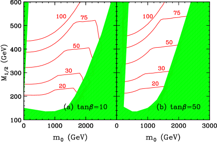
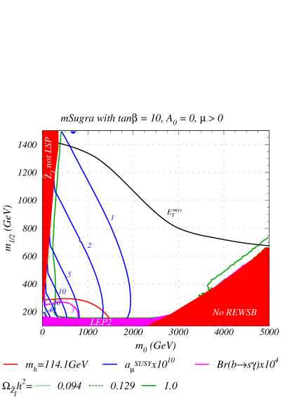
Figure 4: (a) Left panel: Allowed region with different amount of fine-tuning [20]. (b) Right panel: Only little is allowed [21] after including WMAP data.

Now we consider a specific example of fine-tuning in the context of minimal supergravity. In this case, Eq. (13) can be recast in the form

$$M_{Z}^{2}\simeq-2|\mu^{2}|+\frac{3}{2\pi^{2}}h_{t}^{2}m_{\tilde{t}}^{2}\ln\left(\frac{M_{\rm Pl}}{m_{\tilde{t}}}\right)=-2|\mu^{2}|+{\cal{O}}(1)~{}m_{\tilde{t}}^{2}.$$ (15)

The ‘natural’ expectation, i.e. without any fine-tuning, would be $M_{Z}\sim\mu\sim m_{\tilde{t}}$. On the other hand, the radiatively corrected Higgs mass in Eq. (12) takes the approximate form

$$m_{h}^{2}\simeq M_{Z}^{2}+\frac{3h_{t}^{2}}{2\pi^{2}}m_{t}^{2}\ln\left(\frac{m_{\tilde{t}}}{m_{t}}\right).$$ (16)

Now, since $m_{h}>114.4$ GeV, it automatically follows $m_{\tilde{t}}>1$ TeV, contradicting the expectation from ‘naturalness’, and implying a fine-tuning or cancellation among unrelated parameters to the tune of a few percent. This is called the ‘little hierarchy’ problem of supersymmetry. But ‘little hierarchy’ is after all a ‘little’ hierarchy. At least, supersymmetry solves the ‘gauge hierarchy problem’ narrated earlier.

Figs. 4a and 4b refer to minimal supergravity. The left panel [20] shows different contours for different values of the fine-tuning parameter $\Delta$. The contour for $\Delta=100$ admits a cancellation as low as ($1/\Delta=$) 1%, so it allows more parameter space than the more conservative $\Delta=20$ curve which does not admit cancellation below 5%. The right panel shows that minimal supergravity is getting increasingly squeezed as more data pour in. The WMAP data, in particular, select out only a tiny region in the parameter space (for a detailed description of this plot, see [21]). Relaxing certain assumptions would definitely admit more parameter space.

IV Little Higgs

In Nature, we have seen light scalars before – e.g. the pions – though they are composite. Their lightness owes to their pseudo-Goldstone nature. These are Goldstone bosons which arise when the chiral symmetry group ${\rm SU(2)}_{L}\times{\rm SU(2)}_{R}$ spontaneously breaks to the isospin group ${\rm SU(2)}_{I}$. A Goldstone scalar $\phi$ has a shift symmetry $\phi\to\phi+c$, where $c$ is a constant, so any interaction which couples $\phi$ not as $\partial_{\mu}\phi$ will break the Goldstone symmetry and attribute mass to previously massless Goldstone. Quark masses and electromagnetic interaction explicitly break the chiral symmetry. Electromagnetism attributes a mass to $\pi^{+}$ of order $m_{\pi^{+}}^{2}\sim(\alpha_{\rm em}/4\pi)\Lambda_{\rm QCD}^{2}$. Suppose, we conceive Higgs as a composite object, a pseudo-Goldstone of some symmetry, and try to think of its mass generation in the pion theme. We know that Yukawa interaction has a non-derivative Higgs coupling, so it will break the Goldstone symmetry. Then, by analytic continuation, if we replace $\alpha_{\rm em}$ by $\alpha_{\rm top}$ and $\Lambda_{\rm QCD}$ by some $\Lambda_{\rm NP}$, we obtain $m_{h}^{2}\sim(\alpha_{\rm top}/4\pi)\Lambda_{\rm NP}^{2}$. The question is whether this picture is phenomenologically acceptable. The answer is ‘no’, as a $\sim$ 100 GeV Higgs would imply $\Lambda_{\rm NP}\sim 1$ TeV. Such a low cutoff is strongly disfavoured by EWPT.

The little Higgs creators [22] had further tricks up their sleeves to counter this obstacle. Consider the following all-order expansion in coupling constants [4]:

$$m_{h}^{2}=\left(C_{i}\frac{\alpha_{i}}{4\pi}+{C_{i}C_{j}\frac{\alpha_{i}\alpha_{j}}{(4\pi)^{2}}}+\cdot\cdot\right)~{}\Lambda_{\rm NP}^{2}\,.$$ (17)

Here, $\alpha_{i}$ are couplings of some external sources, e.g. gauge or Yukawa interactions, that have nontrivial transformations under the Goldstone symmetry. The coefficients $c_{i}$, $c_{ij}$ are symmetry factors. But now one has to make such a smart choice of gauge groups and representation of scalars that if any of the couplings ($\alpha_{i}$) vanishes the global symmetry is partially restrored. Thus, to totally destroy the global symmetry one requires the combined effect of at least two couplings. Then the Goldstone acquires mass parametrically at the 2-loop level:

$$m_{h}^{2}\sim\left(\frac{\alpha}{4\pi}\right)^{2}\Lambda_{\rm NP}^{2}\,.$$ (18)

This is the concept of collective symmetry breaking. Now, one can think of new physics appearing at $\Lambda_{\rm NP}\sim$ 10 TeV scale. In a sense, this is nothing but a postponement of the problem as the cutoff of the theory is now 10 TeV instead of 1 TeV.

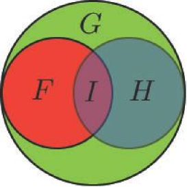
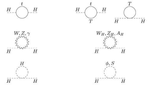
Figure 5: (a) Left panel: A cartoon of little Higgs trick [3]. (b) Right panel: Cancellation between same statistics graphs [3].

To appreciate the little Higgs trick we look into Fig. 5 (left panel). Consider a global group $G$ which spontaneously breaks to $H$ at a scale $f$. The origin of this symmetry breaking is irrelevant below the cutoff scale $\Lambda\sim 4\pi f$. $H$ must contain SU(2) $\times$ U(1) as a subgroup so that when a part of $G$, labelled $F$, is weakly gauged the unbroken SM group, $I$, results. The Higgs – inside the doublet ($h$) under the SM group - is a part of the Goldstone multiplet which parametrizes the coset space $G/H$. For instance, G/H $=$ SU(5)/SO(5) scenario is called the ‘littlest’, while G/H $={\rm SU(3)}^{2}/{\rm SU(2)}^{2}$ scenario is called the ‘simplest’. It is important to note that the generators of the gauged part of $G$ do not commute with the generators corresponding to the Higgs, and thus gauge (as well as Yukawa) interactions break the Goldstone symmetry and induce Higgs mass at one-loop level (parametrically at two-loop order, as we explained before). A clever construction of a little Higgs theory should have the following form of the electroweak sector Higgs potential:

$$V=-\mu^{2}(h^{\dagger}h)+\lambda(h^{\dagger}h)^{2},$$

where, the bilinear term is suppressed, $\mu^{2}\sim\frac{g^{4}}{16\pi^{2}}f^{2}\ln(\Lambda^{2}/f^{2})$, but, crucially, the quartic interaction should be unsuppressed, $\lambda\sim g^{2}$.

Since the gauge group is expanded, we have additional gauge bosons and fermions. With the Higgs boson on external lines of a 2-point function, the quadratic divergence arising from a $Z$-boson loop cancels against the same from a $Z^{\prime}$-boson loop; similar cancellation happens between a $t$-quark loop and a $t^{\prime}$-quark loop (see the right panel of Fig. 5). But the vev $f$ receives a quadratic correction, $f^{2}\to F^{2}=f^{2}+(a/16\pi^{2})\Lambda^{2}=(1+a)f^{2}$, where $a\sim{\cal{O}}(1)$. Thus, $m_{h}^{2}=(g^{4}/16\pi^{2})F^{2}\ln(\Lambda^{2}/F^{2})$, where the quadratic sensitivity is shunned by a loop suppression factor compared to the SM and this is where we gain [2]. Clearly, $f\sim F\sim 1$ TeV. The cutoff of the theory then becomes $\Lambda\sim 4\pi f$, which is 10 TeV (compared to 1 TeV in the SM where naturalness breaks down). The ‘smoking gun’ signals will constitute a few weakly coupled particles (gauge bosons, top-like quark and a scalar coupled to the Higgs) around $f\sim$ TeV.

It is worthwhile to compare and contrast supersymmetry and little Higgs:

Symmetry: In supersymmetry, quadratic divergence to Higgs mass-square cancels between loop diagrams containing different spin particles. In little Higgs models, the above cancellation occurs between loop diagrams with same spin particles. Although the quadratic sensitivity comes back through $f$, it is accompanied by an extra suppression factor in the Higgs mass, which implies that naturalness breaks down at $\sim$ 10 TeV. For ultraviolet (UV) completion, one can either arrange successive little Higgs mechanisms to push the naturalness scale further away, or, perhaps, appeal to supersymmetry or technicolour to come in rescue at 10 TeV [2].

The minus sign: In supersymmetry, large $h_{t}$ drives $m_{H_{u}^{2}}$ negative triggering EWSB. In little Higgs models, too, large $h_{t}$ can generate the desired ‘negative sign’.

Fine-tuning: $m_{h}>114.4$ GeV requires large stop mass, causing the ‘LEP paradox’, leading to ‘little Hierarchy’. In the next-to-minimal MSSM, there is an extra singlet which helps to ease this tension. In little Higgs constructions, suppression of bilinear term compared to quartic term requires fine-tuning in a large class of models.

Dark Matter: The lightest supersymmetric particle (e.g. the lightest neutralino) is an excellent dark matter candidate if $R$-parity is exact. In little Higgs models (the ‘littlest’ type), one can define a $T$-parity to distinguish between the SM particles ($T$-even) and the extra species ($T$-odd). If $T$-parity is conserved, then the lightest $T$-odd gauge boson is cosmologically stable and can act as a good dark matter candidate.

V Gauge-Higgs unification

The basic idea of Gauge-Higgs unification (GHU) is that the Higgs arises from the internal components of a higher dimensional gauge field. Thus higher dimensional gauge invariance provides a protection to the Higgs mass from quadratic divergence. When the extra coordinate is not simply connected (e.g. $S^{1}$), there are Wilson line phases associated with the extra dimensional component of the gauge field, conceptually similar to Aharanov-Bohm phase in quantum mechanics. Their 4d fluctuation is identified with the Higgs. There is no potential at the tree level, only through radiative effects the Higgs boson acquires a mass. The basic steps of understanding the GHU mechanism are as follows:

($i$)  From a 4d point of view, a 5d gauge field $A_{M}$ can be decomposed as $(A_{\mu},A_{5})$, where $\mu=0,1,2,3$. The idea is to relate $A_{5}$ to the Higgs. Consider a simple example: 5d QED on $S^{1}/Z_{2}$. From a 4d point of view, the 5th component of the gauge field is indeed a scalar, and there are $n$ such scalars, $A_{5}^{(n)}$. But none of these $A_{5}^{(n)}$ survives as a physical state. Each of them is ‘eaten up’ by the corresponding $A_{\mu}^{(n)}$, and the latter becomes massive.

($ii$)  Now take SU(3) as a gauge group and choose an orbifold projection $P~{}=~{}{\rm diag}~{}(-1,-1,1)$ (in fundamental rep.) which breaks SU(3) to SU(2) $\times$ U(1).

Denote the SU(3) generators by $T^{a}$ where $a=1,...,8$. Now, with a $Z_{2}$ projection, impose the conditions that the Lie-algebra valued $A_{\mu}\equiv A_{\mu}^{a}T_{a}$ and $A_{5}\equiv A_{5}^{a}T_{a}$ fields transform as $PA_{\mu}P^{\dagger}=A_{\mu}$ and $PA_{5}P^{\dagger}=-A_{5}$.

Due to the relative minus sign between the two sets of transformations, while the massless gauge bosons would transform in the adjoint of SU(2) $\times$ U(1), the massless scalars would behave as a complex doublet under SU(2) $\times$ U(1). This complex doublet can be identified with our Higgs doublet.

($iii$)  Indeed, the next question is how to generate the scalar potential for electroweak breaking. The shift symmetry of the scalar $A_{5}$ fields (i.e., the higher dimensional gauge invariance) forbids us to write this potential at the tree level.

($iv$)  The interaction of the Higgs with bulk fermions and gauge bosons will generate an effective scalar potential at one-loop level. The gauge loops tend to push $\langle A_{5}^{0}\rangle$ to zero to minimize the potential, while the fermionic loops tends to shift $\langle A_{5}^{0}\rangle$ away from zero in the minimum of the potential. In fact, the KK fermions are instrumental for generating the correct vev. This way of breaking SU(2) $\times$ U(1) symmetry to U(1)_em is called the Hosotani mechanism [23]. The one-loop Higgs mass is given by

$$m_{h}^{2}\sim\frac{g^{4}}{128\pi^{6}}\frac{1}{R^{2}}\sum V^{\prime\prime}(\alpha),$$ (19)

where $\alpha$ is a dimensionless parameter arising from bulk interactions, and the sum is over all KK particles. Clearly, 5d gauge symmetry is recovered when $1/R\to 0$.

($v$)  A snapshot of the gauge spectrum is the following:

$$M_{W}^{(n)}=(n+\alpha)/R,~{}~{}M_{Z}^{(n)}=(n+2\alpha)/R,~{}~{}M_{\gamma}^{(n)}=n/R.$$ (20)

The periodicity property demands that the spectrum will remain invariant under $\alpha\to\alpha+1$. This restricts $\alpha=[0,1]$. Orbifolding further reduces it to $\alpha=[0,0.5]$. In principle, $\alpha$ can be fixed from the $W$ mass.

Admittedly, the above scenario does not phenomenologically work as it gives $M_{Z}^{(0)}=2M_{W}^{(0)}$. Yet, it provides an excellent illustration, providing clues to the right direction!

We face some difficult obstacles while constructing a realistic scenario. The GHU models often lead to ($a$) too small a top quark mass, ($b$) too small a Higgs mass, and ($c$) too low a compactification scale. Besides, one has also to worry about how to generate hierarchical Yukawa interaction starting from higher dimensional gauge interaction which is after all universal. One way out is to break the 5d Lorentz symmetry in the bulk:

$$L_{g} = -\frac{1}{4}F_{\mu\nu}F^{\mu\nu}-\frac{\mathbf{a}}{4}F_{\mu 5}F^{\mu 5}~{}~{};~{}~{}L_{\Psi}=\bar{\Psi}\left(i\gamma_{\mu}D^{\mu}-{\mathbf{k}}D_{5}\gamma^{5}\right)\Psi\,,$$ (21)

where the prefactors ${\mathbf{a}}$ and ${\mathbf{k}}$ need to be phenomenologically tuned to match the data. For detailed constructions of gauge-Higgs unification scenarios, both in flat and warped space, we refer the readers to Refs. [24].

VI Higgsless scenarios

The idea is to trigger electroweak symmetry breaking without actually having a physical Higgs. The mechanism relies on imposing different boundary conditions (BC) on gauge fields in an extra-dimensional set-up. The BCs can be carefully chosen such that the rank of a gauge group can be lowered. The details can be found in [25, 26, 27]. Here, we summarise the essentials through the following steps:

($i$)  The simplest realisation is through the compactification of the extra dimension on a circle with an orbifolding ($S^{1}/Z_{2}$). There are two fixed points: $y=0,\pi R$.

($ii$)  BC’s: In general, $\partial_{5}A_{\mu}^{a}=VA_{\mu}^{a}$, where $V$ is the vev of a scalar field in a boundary. If $V=0$ (called ‘Neumann BC’), then $\partial_{5}A_{\mu}^{a}=0$. On the other hand, $V\to\infty$ (called ‘Dirichlet BC’) gives $A_{\mu}^{a}=0$. So, some kind of a Higgs-like mechanism, characterzied by $V$, is there in the backdrop, although eventually the gauge bosons masses following EWSB induced by BC’s would remain finite even in the extreme limits of $V=0$ or $\infty$.

($iii$)  Appropriate BCs are chosen (for explicit formulae, see [26]) which would ensure the following gauge symmetry in bulk and in the two branes:
Bulk:   ${\rm SU(2)}_{\rm L}\times{\rm SU(2)}_{\rm R}\times{\rm U(1)}_{\rm B-L}$   ,
$y=0$ brane:   ${\rm SU(2)}_{\rm L}\times{\rm SU(2)}_{\rm R}\to{\rm SU(2)}_{\rm D}$   ,
$y=\pi R$ brane  : ${\rm SU(2)}_{\rm R}\times{\rm U(1)}_{\rm B-L}\to{\rm U(1)}_{\rm Y}$   .

($iv$)  The gauge boson masses would follow from the solutions of the transcendental equations involving $M_{n}$ and $R$. In flat space, the following relations obtain: $M_{\gamma}=0$, $M_{W}=(4R)^{-1}$, $M_{Z}=(\pi R)^{-1}\tan^{-1}\sqrt{1+2g^{\prime 2}/g^{2}}$. But, $\Delta\rho\simeq 0.1$ is quite large! The reason behind this large $\Delta\rho$ is that while the custodial symmetry is preserved in the bulk and at the $y=0$ brane, it is violated at the $y=\pi R$ brane where the KK modes of the gauge fields have sizable presence. One way out is to use the AdS/CFT correspondence in a warped space. Yet, in the above flat space example, relating the gauge boson masses to the gauge couplings is quite an achievement and is a step to the right direction.

($v$)  Recall that without a Higgs, unitarity violation would have set in the SM at around a TeV. How do the Higgsless scenarios address this issue? Here, the exchange of KK states retards the energy growth of the $W_{L}$-$W_{L}$ scattering amplitude, postponing the violation of unitarity in a calculable way beyond a TeV. Thus unitarity is kept partially under control. This can be understood from a simple dimensional argument: In 4d, the cutoff is $\Lambda_{4}\sim 4\pi v\sim 1$ TeV. In 5d, the loop factor is $g_{5}^{2}/24\pi^{3}=g_{4}^{2}R/12\pi^{2}$, while the dimensionless quantity would be $g_{4}^{2}ER/12\pi^{2}$. The 5d cutoff is then determined as $\Lambda_{5}\sim 12\pi^{2}/g_{4}^{2}R\sim\Lambda_{4}(3\pi/g_{4}^{2})\sim 10$ TeV, for $1/R\sim v$.

($vi$)  EWPT poses a serious threat to the construction of a realistic Higgsless model [27].

VII Conclusions and Outlook

1.  All the BSM models we have considered are based on calculability. In all cases, the electroweak scale $M_{Z}$ can be expressed in terms of some high scale parameters $a_{i}$, i.e. $M_{Z}=\Lambda_{\rm NP}f(a_{i})$, where $f(a_{i})$ are calculable functions of physical parameters.

2.  The new physics scales originate from different dynamics in different cases: $\Lambda_{\rm SUSY}\sim M_{S}$ (the supersymmetry breaking scale); $\Lambda_{\rm LH}\sim f\sim F$ (the vev of the pre-electroweak Higgsing); $\Lambda_{\rm GHU}\sim R^{-1}$ (the inverse radius of compactification).

3.  In supersymmetry, the cutoff can be as high as the GUT or the Planck scale. Both in little Higgs models and in the extra dimensional scenarios (in general) the cutoff is much lower. In fact, in recent years there is a revival of interest in strongly interacting light Higgs models [28]. However, their ultraviolet completion is an open question!

4.  In supersymmetry the cancellation of quadratic divergence happens between a particle loop and a sparticle loop. Since a particle cannot mix with a sparticle, the oblique electroweak corrections and the $Zb\bar{b}$ vertex can be kept under control. In the relevant non-supersymmetric scenarios, the cancellation occurs between loops with the same spin states. Such states can mix among themselves, leading to dangerous tree level contributions that EWPT either disapprove or, at best, marginally admit.

5.  Our goal is three-fold: (i) unitarize the theory, (ii) sucessfully confront the EWPT, and (iii) maintain naturalness to the extent possible. The tension arises as ‘naturalness’ demands the spectrum to be compressed, while ‘EWPT compatibility’ pushes the new states away from the SM states.

6.  All said and done, the LHC is a ‘win-win’ machine in terms of discovery. Either we discover the Higgs, or, if it is not there, the new resonances which would restore unitarity in gauge boson scattering are crying out for verification. For the latter, we would need the super-LHC to cover the entire parameter space. In either scenario, we would need a linear collider for precision studies.

Acknowledgements:  I thank the organizers for inviting me to give this talk. I also thank Romesh Kaul for sharing his insights, particularly in little Higgs models. I acknowledge hospitality at LPT-UMR 8627, Univ. of Paris-Sud 11, Orsay, France, through a CNRS fellowship when this review is being written up. This work is partially supported by the project No. 2007/37/9/BRNS of BRNS (DAE), India.

References

- [1] G. Altarelli, “New Physics and the LHC,” arXiv:0805.1992 [hep-ph]; R. Barbieri, “Signatures of new physics at 14 TeV,” arXiv:0802.3988 [hep-ph]; G. F. Giudice, “Theories for the Fermi Scale,” J. Phys. Conf. Ser. 110 (2008) 012014 [arXiv:0710.3294 [hep-ph]]; R. Barbieri, “Searching for new physics at future accelerators,” Int. J. Mod. Phys. A 20 (2005) 5184 [arXiv:hep-ph/0410223]
- [2] R. K. Kaul, arXiv:0803.0381 [hep-ph].
- [3] H. C. Cheng, arXiv:0710.3407 [hep-ph].
- [4] R. Rattazzi, PoS HEP2005 (2006) 399 [arXiv:hep-ph/0607058].
- [5] LEP Electroweak Working Group, http://lepewwg.web.cern.ch.
- [6] B. W. Lee, C. Quigg and H. B. Thacker, Phys. Rev. D 16 (1977) 1519.
- [7] G. Altarelli and G. Isidori, Phys. Lett. B 337 (1994) 141.
- [8] C. F. Kolda and H. Murayama, JHEP 0007 (2000) 035 [arXiv:hep-ph/0003170].
-
[9]
See the text books on supersymmetry,
R.N. Mohapatra, ‘Unification and Supersymmetry: The Frontiers of quark-lepton physics’, Springer-Verlag, NY 1992; M. Drees, R. Godbole and P. Roy, ‘Theory and phenomenology of sparticles: An account of four-dimensional N=1 supersymmetry in high energy physics,’ World Scientific (2004); H. Baer and X. Tata, ‘Weak scale supersymmetry: From superfields to scattering events,’ Cambridge, UK: Univ. Pr. (2006). -
[10]
For reviews on supersymmetry phenomenology, see for example,
S.P. Martin, hep-ph/9709356; J.D. Lykken, hep-th/9612114; P. Ramond, hep-th/9412234; J. Bagger, hep-ph/9604232; M. Drees, hep-ph/9611409; S. Dawson, hep-ph/9612229; J.F. Gunion, hep-ph/9704349; X. Tata, hep-ph/9706307; J. Louis, I. Brunner, S.J. Huber, hep-ph/9811341; N. Polonsky, hep-ph/0108236; I. Simonsen, hep-ph/9506369; H.E. Haber, hep-ph/0103095; A. Djouadi, Phys. Rept. 459 (2008) 1 [arXiv:hep-ph/0503173]; G. Bhattacharyya, hep-ph/0108267. - [11] For a discussion, see also, L. Hall, ‘The heavy top quark and supersymmetry’, hep-ph/9605258.
- [12] E. Witten, Nucl. Phys. B 188 (1981) 513; S. Dimopoulos, H. Georgi, Nucl. Phys. B 193 (1981) 150; N. Sakai, Z. Phys. C 11 (1981) 153; R.K. Kaul, Phys. Lett. 109 B (1982) 19; R.K. Kaul, P. Majumdar, Nucl. Phys. B 199 (1982) 36.
- [13] J. Ellis, S. Kelley, D.V. Nanopoulos, Phys. Lett. B 260 (1991) 131; U. Amaldi, W. de Boer, H. Furstenau, Phys. Lett. B 260 (1991) 447.
- [14] G. Hinshaw et al. [WMAP Collaboration], arXiv:0803.0732 [astro-ph].
- [15] H. Haber, G. Kane, Phys. Rept. 117 (1985) 75; H.P. Nilles, Phys. Rept. 110 (1984) 1.
- [16] S. Dimopoulos, D.W. Sutter, Nucl. Phys. B 452 (1995) 496.
- [17] R. Barbier et al., Phys. Rept. 420 (2005) 1 [arXiv:hep-ph/0406039]; G. Bhattacharyya, arXiv:hep-ph/9709395; G. Bhattacharyya, Nucl. Phys. Proc. Suppl. 52A (1997) 83 [arXiv:hep-ph/9608415].
- [18] J. R. Ellis, G. Ridolfi and F. Zwirner, Phys. Lett. B 257 (1991) 83 and Phys. Lett. B 262 (1991) 477; Y. Okada, M. Yamaguchi and T. Yanagida, Prog. Theor. Phys. 85 (1991) 1; H. E. Haber and R. Hempfling, Phys. Rev. Lett. 66 (1991) 1815; A. Brignole, Phys. Lett. B 281 (1992) 284; M. S. Berger, Phys. Rev. D41 (1990) 225; J. F. Gunion and A. Turski, Phys. Rev. D39 (1989) 2701; M. Carena, J. R. Espinosa, M. Quiros and C. E. M. Wagner, Phys. Lett. B 355 (1995) 209 [arXiv:hep-ph/9504316]; M. Carena, M. Quiros and C. E. M. Wagner, Nucl. Phys. B 461 (1996) 407 [arXiv:hep-ph/9508343]; H. E. Haber, R. Hempfling and A. H. Hoang, Z. Phys. C 75 (1997) 539 [arXiv:hep-ph/9609331]; S. Heinemeyer, W. Hollik and G. Weiglein, Eur. Phys. J. C 9 (1999) 343 [arXiv:hep-ph/9812472].
- [19] R. Barbieri, G.F. Giudice, Nucl. Phys. B 306 (1988) 63; G. Anderson, G. Castano, Phys. Rev. D 52 (1995) 1693; S. Dimopoulos, G.F. Giudice, Phys. Lett. B 357 (1995) 573; G. Bhattacharyya, A. Romanino, Phys. Rev. D 55 (1997) 7015; P. Ciafaloni, A. Strumia, Nucl. Phys. B 494 (1997) 41; L. Giusti, A. Romanino, A. Strumia, Nucl. Phys. B 550 (1999) 3. See also, G. F. Giudice, arXiv:0801.2562 [hep-ph].
- [20] J. L. Feng, K. T. Matchev and T. Moroi, Phys. Rev. D 61 (2000) 075005 [arXiv:hep-ph/9909334].
- [21] H. Baer, C. Balazs, A. Belyaev, T. Krupovnickas and X. Tata, JHEP 0306 (2003) 054 [arXiv:hep-ph/0304303].
- [22] N. Arkani-Hamed, A. G. Cohen, E. Katz and A. E. Nelson, JHEP 0207 (2002) 034 [arXiv:hep-ph/0206021]; N. Arkani-Hamed, A. G. Cohen, E. Katz, A. E. Nelson, T. Gregoire and J. G. Wacker, JHEP 0208 (2002) 021 [arXiv:hep-ph/0206020]; N. Arkani-Hamed, A. G. Cohen, T. Gregoire and J. G. Wacker, JHEP 0208 (2002) 020 [arXiv:hep-ph/0202089]; N. Arkani-Hamed, A. G. Cohen and H. Georgi, Phys. Lett. B 513 (2001) 232 [arXiv:hep-ph/0105239]; D. E. Kaplan and M. Schmaltz, JHEP 0310 (2003) 039 [arXiv:hep-ph/0302049]; D. E. Kaplan, M. Schmaltz and W. Skiba, Phys. Rev. D 70 (2004) 075009 [arXiv:hep-ph/0405257]; M. Schmaltz, JHEP 0408 (2004) 056 [arXiv:hep-ph/0407143]; M. Schmaltz and D. Tucker-Smith, Ann. Rev. Nucl. Part. Sci. 55 (2005) 229 [arXiv:hep-ph/0502182].
- [23] Y. Hosotani, Phys. Lett. B 126 (1983) 309.
- [24] N. Haba, S. Matsumoto, N. Okada and T. Yamashita, arXiv:0802.3431 [hep-ph]; M. Carena, A. D. Medina, B. Panes, N. R. Shah and C. E. M. Wagner, Phys. Rev. D 77 (2008) 076003 [arXiv:0712.0095 [hep-ph]]; G. Cacciapaglia, C. Csaki and S. C. Park, JHEP 0603 (2006) 099 [arXiv:hep-ph/0510366]; G. Panico, M. Serone and A. Wulzer, Nucl. Phys. B 739 (2006) 186 [arXiv:hep-ph/0510373].
- [25] For a review, see C. Csaki, J. Hubisz and P. Meade, arXiv:hep-ph/0510275.
- [26] C. Csaki, C. Grojean, L. Pilo and J. Terning, Phys. Rev. Lett. 92 (2004) 101802 [arXiv:hep-ph/0308038]; C. Csaki, C. Grojean, H. Murayama, L. Pilo and J. Terning, Phys. Rev. D 69 (2004) 055006 [arXiv:hep-ph/0305237]; C. Csaki, C. Grojean, J. Hubisz, Y. Shirman and J. Terning, Phys. Rev. D 70 (2004) 015012 [arXiv:hep-ph/0310355].
- [27] R. Barbieri, A. Pomarol and R. Rattazzi, Phys. Lett. B 591 (2004) 141 [arXiv:hep-ph/0310285]; G. Cacciapaglia, C. Csaki, C. Grojean and J. Terning, Phys. Rev. D 71 (2005) 035015 [arXiv:hep-ph/0409126]; G. Cacciapaglia, C. Csaki, C. Grojean and J. Terning, Phys. Rev. D 70 (2004) 075014 [arXiv:hep-ph/0401160].
- [28] G. F. Giudice, C. Grojean, A. Pomarol and R. Rattazzi, JHEP 0706 (2007) 045 [arXiv:hep-ph/0703164].