$N$-body + Magnetohydrodynamical Simulations of Merging Clusters of Galaxies: Characteristic Magnetic Field Structures Generated by Bulk Flow Motion

Abstract

We present results from $N$-body + magnetohydrodynamical simulations of merging clusters of galaxies. We find that cluster mergers cause various characteristic magnetic field structures because of the strong bulk flows in the intracluster medium. The moving substructures result in cool regions surrounded by the magnetic field. These will be recognized as magnetized cold fronts in the observational point of view. A relatively ordered magnetic field structure is generated just behind the moving substructure. Eddy-like field configurations are also formed by Kelvin-Helmholtz instabilities. These features are similarly seen even in off-center mergers though the detailed structures change slightly. The above-mentioned characteristic magnetic field structures are partly recognized in Faraday rotation measure maps. The higher absolute values of the rotation measure are expected when observed along the collision axis, because of the elongated density distribution and relatively ordered field structure along the axis. The rotation measure maps on the cosmic microwave background radiation, which covers clusters entirely, could be useful probes of not only the magnetic field structures but also the internal dynamics of the intracluster medium.

1 Introduction

Clusters of galaxies have plenty of hot plasma as well as galaxies and dark matter (DM), which is called intracluster medium (ICM). Some observational evidence indicates that ICM is magnetized. For example, some clusters have diffuse non-thermal synchrotron radio emission that is called radio halos or relics, which shows that there are magnetic fields as well as relativistic electrons in the intracluster space (Giovannini et al., 1999; Kempner & Sarazin, 2001). In addition, Faraday rotation measure observations of polarized radio sources such as radio lobes and AGNs behind and/or in clusters indicate that the magnetic field structures are quite random (Clarke et al., 2001; Vogt & Ensslin, 2003; Govoni et al., 2006).

Comparing the synchrotron radio flux with the hard X-ray one (or its upper limit) due to the inverse Compton scatterings of cosmic microwave background (CMB) photons, we are able to estimate the volume averaged magnetic field strength (or its lower limit). Typically, the strength of $\sim 0.1\mu$G is obtained with this method (Fusco-Femiano et al., 1999, 2005) though those detections of non-thermal hard X-ray components are still controversial (Rossetti, & Molendi, 2004; Fusco-Femiano et al., 2007). On the other hand, somewhat higher values ($\sim$ a several $\mu$G) tend to be obtained with the Faraday rotation measure method (Clarke et al., 2001; Vogt & Ensslin, 2003; Govoni et al., 2006) though these results depend on the detailed magnetic field structures that are not fully understood (Ensslin & Vogt, 2003; Murgia et al., 2004).

Although the magnetic energy density is typically $\sim$ a few percents of the thermal one in the intracluster space, it is believed that the magnetic fields play a crucial role in various aspects of ICM. It is likely that non-thermal particles are accelerated via shocks (Sarazin, 1999; Takizawa & Naito, 2000; Totani & Kitayama, 2000; Miniati et al., 2001; Ryu et al., 2003; Takizawa, 2003; Inoue et al., 2005) and/or turbulence (Roland, 1981; Schlickeiser et al., 1987; Blasi, 2000; Ohno et al., 2002; Fujita et al., 2003; Brunetti et al., 2004), where the magnetic fields play a definitive role in most theoretical models of the particle acceleration. Heat conduction is probably depends on the magnetic field configurations because charged particles cannot freely move in the direction perpendicular to the field lines. As we wrote before, magnetic field seems to be a minor component in global ICM dynamics. However, it is possibly important in relatively small scales, where fluid instabilities such as Rayleigh-Taylor and Kelvin-Helmholtz ones might be suppressed by magnetic tension.

Cluster mergers have a significant impact on ICM magnetic field evolution. Turbulent motion excited by mergers would amplify the field strength via dynamo mechanism. Moving substructures are expected to sweep the field lines and form the cold subclumps surrounded by the field lines (Vikhlinin et al., 2001). Asai et al. (2004) and Asai et al. (2007) performed two and three dimensional magnetohydrodynamical(MHD) simulations of moving cold subclumps in hot ICM in rather idealized situations, respectively, which confirmed that expectation. This field structure might be responsible for the suppression of heat conduction and fluid instabilities, which is essential for the maintenance of cold fronts.

A lot of numerical simulations about merging clusters have been done, most of which are $N$-body + hydrodynamical simulations (Roettiger et al., 1996; Takizawa, 1999, 2000; Ricker & Sarazin, 2001; Ritchie & Thomas, 2002; Ascasibar & Markevitch, 2006; Takizawa, 2006; McCarthy et al., 2007; Springel & Farrar, 2007). Although these simulations give us a great deal of understanding of the structures, evolution, and observational implications for merging clusters of galaxies, they make only a limited contribution to investigate the magnetic field structures. MHD simulations are essential in this regard. However, $N$-body + MHD simulations are rather rare though Roettiger et al. (1999) did pioneering work. It is true that Lagrangian particle methods based on smoothed particle hydrodynamics (see Monaghan, 1992) are extensively used in cosmological MHD simulations (Dolag et al., 1999, 2002). Considering that Eulerian mesh codes are essentially better at following evolution of magnetic fields, simulations based on such codes are highly desirable. In this paper, we present the results from $N$-body + MHD simulations of merging clusters of galaxies and investigate characteristic magnetic field structures during mergers and their implications.

The rest of this paper is organized as follows. In §2 we describe the adopted numerical methods and initial conditions for our simulations. In §3 we present the results. In §4 we summarize the results and discuss their implications.

2 The Simulations

2.1 Numerical Methods

Numerical methods used here are basically similar to those in Takizawa (2006) except that ideal MHD equations are calculated for ICM instead of ordinary hydrodynamical ones. In the present study, we consider clusters of galaxies consisting of two components: collisionless particles corresponding to the galaxies and DM, and magnetized gas corresponding to the ICM. When calculating gravity, both components are considered, although the former dominates over the latter. Radiative cooling and heat conduction are not included. In calculating the MHD equations for the ICM, we use a simple linearized Riemann solver originally proposed by Brio & Wu (1988) and introduced into astrophysical MHD simulations by Ryu & Jones (1995). This Riemann solver is a similar and simpler version of Roe’s method (Roe, 1981). Using the MUSCLE approach and a minmod TVD limiter (see Hirsch, 1990), we obtain second-order accuracy without any numerical oscillations around discontinuities. To avoid negative pressure, we solve the equations for the total energy and entropy conservation simultaneously. This method is often used in astrophysical hydrodynamic simulations where high Mach number flow can occur (Ryu et al., 1993; Wada & Norman, 2001).

Gravitational forces are calculated by the Particle-Mesh (PM) method with the standard Fast Fourier Transform technique for the isolated boundary conditions (see Hockney & Eastwood, 1988). The size of the simulation box is $(9.44\,\mathrm{Mpc})^{3}$. For typical runs, the number of the grid points is $(256)^{3}$, and total number of the $N$-body particles is $(128)^{3}$, which is approximately $2.1\times 10^{6}$.

2.2 An Equilibrium Cluster Model

We consider mergers of two virialized subclusters with an NFW density profile (Navarro et al., 1997) in the $\Lambda$CDM universe ($\Omega_{0}=0.25$, $\lambda_{0}=0.75$) for DM,

$$\rho_{\rm DM}(r)=\frac{\delta_{\rm c}\rho_{\rm crit}}{(r/r_{\rm s})(1+r/r_{\rm s})^{2}},$$ (1)

where $\delta_{\rm c}$, $\rho_{\rm crit}$, and $r_{\rm s}$ are the characteristic (dimensionless) density, critical density, and scale radius, respectively. Given the cosmological parameters and halo’s virial mass, we calculate these parameters following a method in Appendix of Navarro et al. (1997).

The initial density profiles of the ICM are assumed to be those of a beta-model,

$$\rho_{\rm gas}(r)=\rho_{\rm gas,0}\biggl{\{}1+\biggl{(}\frac{r}{r_{\rm c}}\biggr{)}\biggr{\}}^{-3\beta/2},$$ (2)

where $\rho_{\rm gas,0}$ and $r_{\rm c}$ are the central gas density and core radius, respectively. We assume that $\beta=0.6$, which is consistent with typical values obtained form the recent X-ray observations (Vikhlinin et al., 2006; Croston et al., 2008). On the other hand, it is not easy to obtain the observational relationship between $r_{\rm c}$ and $r_{\rm s}$ considering difficulty of accurate determination of mass profile. Following the discussion in Ricker & Sarazin (2001), therefore, we chose $r_{\rm c}=r_{\rm s}/2$ as a fiducial value. The gas mass fraction is set to be 0.1 inside of the virial radius of each subcluster. It should be noted that the results will not be sensitive to the choice of this fraction unless the ICM dominates the DM in gravity.

The velocity distribution of the DM particles is assumed to be an isotropic Maxwellian. The radial profiles of the DM velocity dispersion are calculated from the Jeans equation with spherical symmetry, so that the DM particles would be in virial equilibrium in the cluster potential of the DM and ICM,

$$\frac{d}{dr}(\rho_{\rm DM}\sigma^{2})=-\frac{GM(r)}{r^{2}}\rho_{\rm DM},$$ (3)

where $\sigma^{2}$ and $M(r)$ are the one dimensional velocity dispersion at $r$ and total mass inside $r$, respectively. $G$ is the gravitational constant. We need boundary conditions to obtain $\sigma^{2}(r)$ from differential equation (3), which is assume to be

$$\sigma^{2}(r_{\rm vir})=\frac{GM(r_{\rm vir})}{3r_{\rm vir}},$$ (4)

where $r_{\rm vir}$ is the virial radius of the halo.

The radial profiles of the ICM pressure are determined in a similar way so that the ICM would be in hydrostatic equilibrium within the cluster potential,

$$\frac{dP}{dr}=-\frac{GM(r)}{r^{2}}\rho_{\rm gas}.$$ (5)

The boundary conditions for equation (5) is

$$P(r_{\rm vir})=\frac{1}{\beta_{\rm spec}}\frac{GM(r_{\rm vir})}{3r_{\rm vir}}\rho_{\rm gas}(r_{\rm vir}),$$ (6)

where $\beta_{\rm spec}$ is the specific energy ratio of the DM and gas at the virial radius. In case of the classical isothermal $\beta$-model (see Sarazin, 1986), $\beta_{\rm spec}$ should be equal to the fitting parameter $\beta$ in equation (2) to obtain isothermal temperature profile. Although our model is different than the isothermal $\beta$ model in underlying DM distribution, we assume $\beta_{\rm spec}$=$\beta$ for simplicity. As a result, the temperature profile is not isothermal.

2.3 Initial Conditions

For typical runs, the DM masses within the virial radius of the larger and smaller subclusters are $5.0\times 10^{14}\,\mbox{${M}_{\odot}$}$ and $1.25\times 10^{14}\,\mbox{${M}_{\odot}$}$, respectively. Thus, the mass ratio is $4:1$. It is useful to introduce an angular momentum parameter $\lambda\equiv J|E|^{1/2}/(GM^{5/2})$ in order to characterize off-center collisions, where $J$, $E$, and $M$ are the angular momentum of the two subclusters around the center of masses, the binding energy between the two, and the total mass, respectively. Please note that $\lambda$ is the ratio between the actual angular velocity and the angular velocity needed to provide rotational support (see Binney & Tremaine, 1987).

Given each subcluster’s mass and an angular momentum parameter of the system, we estimate “typical” initial conditions for cluster mergers in a similar way of Takizawa (1999). How to estimate these conditions is described in detail in Appendix, which is a natural generalization of the method for head-on collisions (see Takizawa, 1999, section 2) to cases including off-center collisions. The coordinate system is taken in such a way that the center of mass is at rest at the origin. Two subclusters are initialized in the $xy$-plane, separated by a distance $\sqrt{(R_{1}+R_{2})^{2}-b^{2}}$ in the $x$-direction, and $b$ in the $y$-direction, where $R_{1,2}$ and $b$ are the virial radii of the each subcluster and the impact parameter, respectively. The initial relative velocity is directed along the $x$-axis. The centers of the larger and smaller subclusters were initially located at the sides of $x<0$ and $x>0$, respectively.

At present, we have only limited information about magnetic field configurations in the intracluster space. Roughly speaking, however, they have random structures whose power spectrum can be approximated by a power-law in a smaller scale, and the mean field strength is an increasing function of the gas density. Taking these features into account, we make the initial magnetic field as follows. First, we generate random Gaussian vector potential in the wave-numbers space with a zero mean and single power-law spectrum, $A(k)\propto k^{-\mu}$. We assume $\mu=5/3$. Then, the generated potential is transformed into the real space using a three-dimensional Fast Fourier Transform and multiplied by a factor of $\rho_{\rm gas}^{2/3}$, which is expected assuming a uniform spherical collapse and flux freezing. A random and divergence-free magnetic field is calculated via $\bm{B}=\bm{\nabla}\times\bm{A}$. The normalization of the magnetic field is determined so that the total magnetic energy is one percent of the thermal one. Strictly speaking, each subcluster in the initial conditions is not in hydrostatic equilibrium with magnetic field. However, it does not a matter in our simulations because the magnetic energy is much less than the thermal one as we wrote above.

The parameters for each model are summarized in table 1, where $M_{i}$, $r_{{\rm s},i}$, $c_{i}$, $N_{i}$ are the total mass, scale radius, concentration parameter, and number of $N$-body particles for the $i$-th subcluster, respectively. $N_{\rm grd}$ is the total number of grid points. RunST, which is a simple head-on collision case with the mass ratio of 4:1, is regard as a standard run. RunOC is a case of an off-center merger with $\lambda=0.05$. RunMM is a relatively minor merger case with the mass ratio of 8:1. RunLR is a lower resolution run to investigate how the results depend on numerical resolution.

3 Results

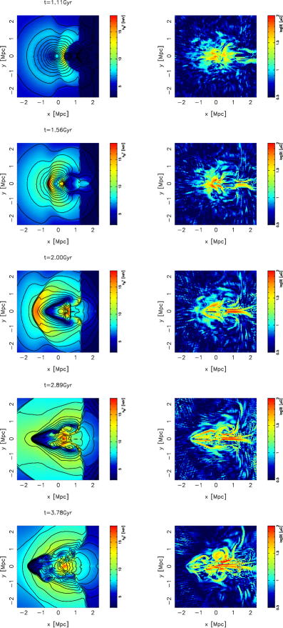
Figure 1: Left: Snapshots of the density (contours) and temperature (colors) distributions on the $z=0$ surface at $t=$1.11, 1.56, 2.00, 2.89, and 3.78 Gyr of RunST. Right: Same, but for the magnetic field strength distribution.

The left panels of Figure 1 show snapshots of the density (contours) and temperature (colors) on the $xy$-plain, which is perpendicular to the collision axis, at $t=1.11$, $1.56$, $2.00$, $2.89$, and $3.78$ Gyr of RunST. Right ones show the same but for the magnetic field strength. At $t=1.11$ Gyr, two subclusters are approaching each other, and temperature between two density peaks is higher than elsewhere. However, magnetic field strength in this region is lower than that in the density peaks. This is simply because initial mean magnetic field strength increase with the density. Although the magnetic field there is slightly amplified by the adiabatic compression, this does not compensate the trend of the initial magnetic field. At $t=1.56$ and $2.0$ Gyr, slightly amplified magnetic field is seen just behind the shock. However, two kinds of structure appear more notably. One is a relatively strong magnetic field region associated with a contact discontinuity between the ICM originated from the smaller and larger subclusters, which will be recognized as a cold front with strong magnetic field in the observational point of view. As a result, a cool region surrounded by the magnetic field appears. The other is an ordered magnetic field in $x$-direction just behind the subcluster. This is because flow behind subcluster is converging on the collision axis. As a result, the magnetic field are collected and amplified because of compression. At $t=2.89$ Gyr, the bow shock has gone outside of the panel. the field structure associated with the contact discontinuity and ordered field along the collision axis are still present. In addition, eddy-like field structures start to appear above and below the ordered field along the collision axis in $xy$-plain. These structures grow as Kelvin-Helmholtz instabilities develop and become clearer at $t=3.78$ Gyr

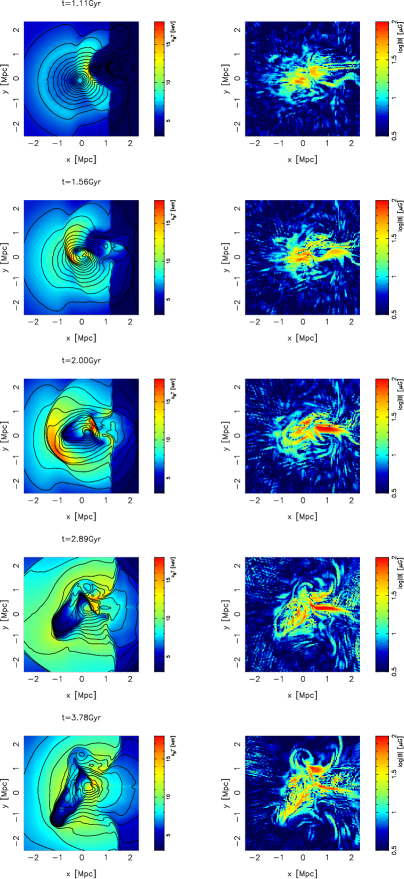
Figure 2: Same as Fig. 1, but for RunOC.

The initial conditions of RunST have an axial symmetric structure. Thus, the above-mentioned features could change significantly in off-center mergers. Figure 2 shows the same as figure 1, but for RunOC. Again, the prominent magnetic structures are associated with a contact discontinuity rather than a bow shock. Because of the asymmetry, the magnetic field at the contact discontinuity is stronger in the side closer to the lager cluster core (or lower side in each panel) at $t=2.00$ and $2.89$ Gyr. A cool region surrounded by the magnetic field certainly appears, but the field structure in the side farther to the larger cluster core (or upper side in each panel) becomes less clear at $t=3.78$ Gyr. As in the case of RunST, an ordered and relatively strong magnetic field structure appears behind the moving substructure. However, this is not just behind the clump but shifted towards the lager cluster side. Eddy-like magnetic fields generated by the Kelvin-Helmholtz instabilities are clearer in the side further to the larger cluster.

Cluster mergers cause various characteristic magnetic field configurations as we see before. Unfortunately, it is very difficult to observe the magnetic field structure itself directly at present. The observation of Faraday rotation measure is an indirect, but quite useful way to obtain information of the magnetic field structure. The rotation measure (RM) is given by (see Rybicki & Lightman, 1979),

$${\rm RM}[{\rm rad}/{\rm m}^{2}]=812\int n_{\rm e}[{\rm cm}^{-3}]B_{||}[\mu{\rm G}]dl,$$ (7)

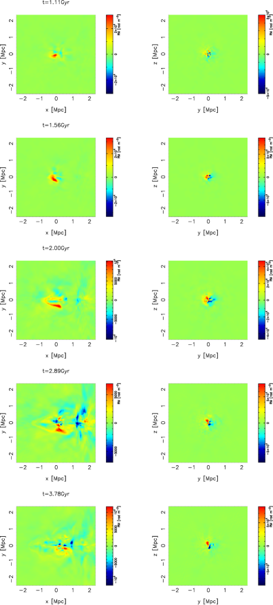
Figure 3: Snapshots of the Faraday rotation measure map of RunST at the same epochs as in Fig 1. Left and right panels show the rotation measure when the line-of-sight is perpendicular and parallel to the collision axis, respectively.

where $n_{\rm e}$ and $B_{||}$ are the electron number density and line-of-sight component of the magnetic field, respectively. Figure 3 presents snapshots of the RM map for RunST. Left and right panels show the maps seen from the $z$ and $x$ axis, respectively. Please remember that the collision axis is along the $x$-axis. When the line-of-sight is perpendicular to the collision axis, RM maps give us relatively rich information. Cool regions with high magnetic field are seen as those with high absolute values of RM. On the other hand, the structure is relatively featureless when we observe the system along the collision-axis. The absolute values of RM tend to be higher in the right panels, which is not surprising because the density distribution is elongated along the collision axis, and because there is the ordered magnetic field in the same direction behind the subclump.

Figure 4 shows profiles along the collision axis at $t=2.00$ Gyr of RunST for (a) pressure, (b) electron number density, (c) temperature, (d) $x$-component of velocity, (e) $x$-component of the magnetic field, and (d) absolute value of the magnetic field perpendicular to the axis. There is a bow shock at $x\simeq-1.5$, where a clear discontinuity are seen in the profiles of pressure, density, temperature, and $x$-component of velocity. A somewhat blunt contact discontinuity is at $x\simeq-1$, where density and temperature have a jump, but pressure and $x$-velocity are smooth. The magnetic field perpendicular to the axis also increase across the bow shock. The tangential magnetic field is amplified between the shock and the contact discontinuity. As a result, the cool region is wrapped by the magnetized layers. This characteristic structure probably have an influence on the transport process such as heat conduction, which will be discussed later.

Because minor mergers are more frequent in actual situations, it is interesting how the results change in minor mergers. Figure 5 shows the same as figure 4 but for RunMM, where mass ratio is 1:8. Mach number of the bow shock becomes lower, which is clearly seen in the profile of pressure, density, temperature, and $x$-component of velocity. As a result, amplification of the magnetic field component perpendicular to the collision axis around contact discontinuity is less prominent, where typical values are roughly halves of those in RunST. On the other hand, typical strength of the $x$-component of the magnetic field does not change very much.

It is possible that our results, especially on the small scale structures around the cold front and bow shock, depend on numerical resolution. To assess this, we perform a lower resolution run as RunLR. Both the numbers of grid points and particles in RunLR are eighths of those in RunST. The initial conditions of RunLR is essentially the same as those of RunST though the largest wave-number components in the magnetic field are not included. Figure 6 shows the same as figure 4 but for RunLR. Although the overall features in pressure, density, temperature, and $x$-component of velocity are similar to those of RunST qualitatively, it is obvious that the width of the contact discontinuity is broader. Width of the bow shock is also slightly broader. As for magnetic field, although the small scale structures disappear, amplification of the field component perpendicular to the collision axis near the contact discontinuity is clearly seen again.

4 Summary and Discussion

We perform $N$-body and MHD simulations of merging clusters of galaxies. We find that cluster mergers cause various characteristic magnetic field structures because of strong bulk flow motion. The magnetic field component perpendicular to the collision axis is amplified especially between a bow shock and contact discontinuity. As a result, a cool region wrapped by the field lines appears. A relatively ordered field structure along the collision axis appears just behind the moving substructure. Eddy-like field structures are also generated by Kelvin-Helmholtz instabilities. Although the detailed structures change slightly, similar features are seen in off-center mergers. RM maps have some information about the magnetic field structure. The above-mentioned characteristic structures are partly recognized in the RM maps when we observe the merging systems in the direction perpendicular to the collision axis. On the other hand, RM maps observed nearly along the collision axis are less informative in this respect. Typical absolute values of the RM become higher when the system is observed along the collision axis because of both the density distribution elongated toward the axis and ordered magnetic field along the same direction. In minor mergers, amplification of the magnetic field component perpendicular to the collision axis becomes less prominent. The results about magnetic field along the collision axis does not change very much. Although numerical resolution effects have the significant impact on the small scale structures such as widths of a bow shock and contact discontinuity and detailed small scale fluctuations of the magnetic field, our results about overall global structures are reasonably reliable.

Some observational and theoretical studies suggest that heat conduction in the ICM is suppressed from the Spitzer value. For example, a sharp temperature jump across a cold front in A2142 requires that the heat conductivity is reduced by a factor of between 250 and 2500 at least in the direction across the front (Ettori & Fabian, 2000). The spatial temperature variations in the central region of A754 also suggest that the conductivity is at least an order of magnitude lower than the Spitzer value (Markevitch et al., 2003). It is well-known that fine-tuning of heat conductivity is necessary in order to reproduce observational natures of cool cores assuming that radiative cooling in the cores balances with the conductive heating from the outer part of the clusters (Zakamska & Narayan, 2003). Although the detailed process involved there is still unclear, magnetic fields likely play an important role. Heat conduction in the direction across the magnetic field lines is likely suppressed because electrons cannot travel freely in that direction. Using two dimensional MHD simulations with anisotropic heat conduction, Asai et al. (2004) shows that a moving subclump naturally form the magnetic field structure along the contact discontinuity and that the temperature jump there is maintained if the heat conduction perpendicular to the field line is sufficiently suppressed. Similar results are obtained in three dimensional cases (Asai et al., 2007). Basically, our simulations confirmed their results about magnetic field configurations in more realistic situations, though the heat conduction is not included.

We show that Faraday rotation measure maps are useful to obtain information about characteristic magnetic field structures formed by cluster mergers. This could be another probe of internal dynamics of clusters. However, there is a serious problem in this method at present. We need polarized radio sources such as radio lobes and/or AGNs in and/or behind the clusters of galaxies to do that. In other words, we are able to obtain RM maps in the limited regions where we have suitable polarized sources by chance. Naturally, these do not always correspond to the regions that we are interested in. However, this difficulty could be overcame if we have suitable polarized sources that covers a cluster entirely. One possible solution is to use the CMB as the polarized source (Ohno et al., 2003), though this is still challenging in the present status of CMB observations. There are a lot of observations that are ongoing and planned for measuring the CMB polarization. We hope that future observations of the CMB polarizations will enable us to make RM maps that cover clusters entirely, which would give us an important clues to understand the internal dynamics as well as the magnetic field structures in clusters of galaxies.

In actual clusters, the magnetic field have random components in small scales. It is very difficult to treat such scales by numerical simulations that concern the global structures. Clearly, observed RM maps are influenced by the small scale magnetic field fluctuations, which are not considered in RM maps calculated from our results. As a result, coherent length of the magnetic fields tends to be overestimated effectively, which means absolute values of RM from the simulations are also overestimated. However, it is probable that global spatial patterns of RM maps are nearly independent of such small scale fluctuations. In addition, it is also probably robust that higher RM are expected when the merging systems are observed along the collision axis.

Appendix A An Estimation Method of the Initial Conditions of Mergers

The estimation method introduced here is a natural extension of that for head-on collisions in Takizawa (1999) to cases including off-center collisions. We consider a merger of two subclusters with masses $M_{1}$ and $M_{2}$ ($M_{1}\geq M_{2}$). Let us consider a region that contains both subclusters. It expands following the cosmological expansion at first. However, the expansion is decelerated and then the region will collapse if the mean density is higher than the critical one. We assume that they are separated by the distance of $2r_{\rm ta}$ at the maximum expansion epoch. In case of head-on collisions, it is obvious that they are at rest for their center of mass at that time. In case of off-center mergers, on the other hand, they have the relative tangential velocity $v_{0}$ at that time. Taking into account the conservation of energy and angular momentum between at the maximum expansion epoch and just before the merger, we obtain following equations,

$$-\frac{GM_{1}M_{2}}{2r_{\rm ta}}+\frac{1}{2}Mv_{0}^{2} = -\frac{GM_{1}M_{2}}{R_{1}+R_{2}}+\frac{1}{2}Mv^{2},$$ (A1)

$$2Mv_{0}r_{\rm ta} = Mvb,$$ (A2)

where $R_{1}$, $R_{2}$, $v$, and $b$ are the virial radius for each subcluster, the initial collision velocity, and the initial impact parameter, respectively. $M\equiv M_{1}M_{2}/(M_{1}+M_{2})$ is the reduced mass of the system. It is natural that the virial radius has correlation with the mass. According to a spherical collapse model, the virial mass is proportional to the square of the virial radius (see Peebles, 1980). Thus, we assume that the following relation,

$$R_{2}=\biggl{(}\frac{M_{2}}{M_{1}}\biggr{)}^{1/3}R_{1}.$$ (A3)

The spherical collapse model also tell us that the turn around radius is twice of the virial radius. Thus, we also assume,

$$r_{\rm ta}=2\biggl{(}\frac{M_{1}+M_{2}}{M_{1}}\biggr{)}^{1/3}R_{1}.$$ (A4)

Using equations (A1), (A2), (A3), and (A4), we eliminate $v_{0}$ and obtain $v$ as follows,

$$v^{2}=\frac{2GM_{1}}{R_{1}}(1+\alpha)\biggl{\{}\frac{1}{1+\alpha^{1/3}}-\frac{1}{4(1+\alpha)^{1/3}}\biggr{\}}\biggl{\{}1-\frac{1}{16(1+\alpha)^{2/3}}\biggl{(}\frac{b}{R_{1}}\biggr{)}^{2}\biggr{\}}^{-1},$$ (A5)

where

$$\alpha\equiv\frac{M_{2}}{M_{1}}.$$ (A7)

It is useful to introduce an angular momentum parameter $\lambda\equiv J|E|^{1/2}/(GM^{5/2})$ in order to characterize off-center mergers, where $J$, $E$, and $M$ are the angular momentum of the two subclusters around the center of masses, the binding energy between the two, and the total mass, respectively. Please note that $\lambda$ is the ratio between the actual angular velocity and the angular velocity needed to provide rotational support (see Binney & Tremaine, 1987).

From equations (A1) and (A2), we obtain

$$\lambda=\frac{vb}{(GM_{1}R_{1})^{1/2}}\frac{\alpha^{3/2}}{(1+\alpha)^{7/2}}\biggl{\{}\frac{1}{1+\alpha^{1/3}}-\frac{R_{1}v^{2}}{2GM_{1}(1+\alpha)}\biggr{\}}^{1/2}.$$ (A8)

Given $M_{1}$, $R_{1}$, $\alpha$, and $\lambda$, therefore, we are able to calculate $v$ and $b$ from equations (A5) and (A8).

Figure 4: Profiles along the $x$-axis at $t=2.00$ Gyr of RunST, for (a)pressure, (b)electron number density, (c)temperature, (d)$x$-component of velocity, (e)$x$-component of magnetic field, and (d)absolute value of magnetic field perpendicular to the $x$-axis, respectively.

Figure 5: Same as Fig. 4, but for RunMM.

Figure 6: Same as Fig. 4, but for RunLR.

Table 1: Model Parameters

Parameters	RunST	RunOC	RunMM	RunLR
$M_{1}/M_{2}(10^{14}\mbox{${M}_{\odot}$})$	5.0/1.25	5.0/1.25	5.0/0.625	5.0/1.25
$r_{{\rm s},1}/r_{{\rm s},2}$ (kpc)	256/139	256/139	256/104	256/139
$c_{1}/c_{2}$	6.12/7.08	6.12/7.08	6.12/7.56	6.12/7.08
$\lambda$	0.0	0.05	0.0	0.0
$N_{1}/N_{2}$	1677721/419431	1677721/419431	1864135/233017	209715/52429
$N_{\rm grd}$	$(256)^{3}$	$(256)^{3}$	$(256)^{3}$	$(128)^{3}$

References

- Ascasibar & Markevitch (2006) Ascasibar, Y., & Markevitch, M. 2006, ApJ, 650, 102
- Asai et al. (2004) Asai, N., Fukuda, N., & Matsumoto, R. 2004, ApJ, 606, L105
- Asai et al. (2007) Asai, N., Fukuda, N., Matsumoto, R. 2007, ApJ, 663, 816
- Binney & Tremaine (1987) Binney, J., & Tremaine, S. 1987, Galactic Dynamics (Princeton: Princeton Univ. Press)
- Blasi (2000) Blasi, P. 2000, ApJ, 532, L9
- Brio & Wu (1988) Brio, M., & Wu, C. C. 1988 J. Comput. Phys., 75 400
- Brunetti et al. (2004) Brunetti, G., Blasi, P., Cassano, R., & Gabici, S. 2004, MNRAS, 350, 1174
- Clarke et al. (2001) Clarke, T., E., Kronberg, P. P., & Böhringer, H. 2001, ApJ, 547, L111
- Croston et al. (2008) Croston, J. H., Pratt, G. W., Boehringer, H., Arnaud, M., Pointecouteau, E., Ponman, T. J., Sanderson, A. J. R., Temple, R. F., Bower, R. G., & Donahue, M. A&A, 2008, in press (arXiv:0801.3430)
- Dolag et al. (1999) Dolag, K., Bartelmann, M., & Lesch, H. A&A, 1999, 348, 351
- Dolag et al. (2002) Dolag, K., Bartelmann, M., & Lesch, H. A&A, 2002, 387, 383
- Ensslin & Vogt (2003) Ensslin, T. A., & Vogt, C. A&A, 2003, 401, 835
- Ettori & Fabian (2000) Ettori, S., & Fabian, A. C. 2000, MNRAS, 317, L57
- Fujita et al. (2003) Fujita, Y., Takizawa, M., & Sarazin, C. L. 2003, ApJ, 584, 190
- Fusco-Femiano et al. (1999) Fusco-Femiano, R., Dal Fiume, D., Feretti, L., Giovannini, G., Grandi, P., Matt, G., Molendi, S., & Santangelo, A. 1999, ApJ, 513, L21
- Fusco-Femiano et al. (2005) Fusco-Femiano, R., Landi, R., Orlandini, M. 2005, ApJ, 624, L69
- Fusco-Femiano et al. (2007) Fusco-Femiano, R., Landi, R., Orlandini, M. 2007, ApJ, 654, L9
- Giovannini et al. (1999) Giovannini, G., Tordi, M., & Feretti, L. 1999, New A, 4, 141
- Govoni et al. (2006) Govoni, F., Murgia, M., Feretti, L., Giovannini, G., Dolag, K., & Taylor G. B. 2006, A&A, 460, 425
- Hirsch (1990) Hirsch, C. 1990, Numerical Computation of Internal and External Flows (New York: John Wiley & Sons)
- Hockney & Eastwood (1988) Hockney, R. W., & Eastwood, J. W. 1988, Computer Simulation Using Particles (London: Institute of Physics Publishing)
- Inoue et al. (2005) Inoue, S., Aharonian, F. A., & Sugiyama, N. 2005, ApJ, 628, L9I
- Kempner & Sarazin (2001) Kempner, J. C., & Sarazin, C. L. 2001, ApJ, 548, 639
- Navarro et al. (1997) Navarro, J. F., Frenk, C. S., & White, S. D. M. 1997, ApJ, 490, 493
- Markevitch et al. (2003) Markevitch, M., Mazzotta, P., Vikhlinin, A., Burke, D., Butt, Y., David, L., Donnelly, H., Forman, W. R., Harris, D., Kim, D.-W., Virani, S., & Vrtilek, J. 2003, ApJ, 586, L19
- McCarthy et al. (2007) McCarthy, I. G., Bower, R. G., Balogh, M. L., Voit, G. M., Pearce, F. R., Theuns, T., Babul, A., Lacey, C. G., & Frenk, C. S. 2007, MNRAS, 376, 497
- Miniati et al. (2001) Miniati, F., Jones, T. W., Kang, H., & Ryu, D. 2001, ApJ, 562, 233
- Monaghan (1992) Monaghan, J. J. 1992 ARA&A, 30, 543
- Murgia et al. (2004) Murgia, M., Govoni, F., Feretti, L., Giovannini, G., Dallacasa, D., Fanti, R., Taylor, G. B., & Dolag, K. 2004, A&A, 424, 429
- Ohno et al. (2002) Ohno, H., Takizawa, M., & Shibata, S. 2002 ApJ, 577, 658
- Ohno et al. (2003) Ohno, H., Takada, M., Dolag, K., Bartelmann, M., & Sugiyama, N. 2003, ApJ, 584, 5990
- Peebles (1980) Peebles, P. J. E. 1980, The Large-Scale Structure of the Universe (Princeton: Princeton Univ. Press)
- Ricker & Sarazin (2001) Ricker, P. M., & Sarazin, C. L. 2001, ApJ, 561, 624
- Ritchie & Thomas (2002) Ritchie, B. W., & Thomas, P. A. 2002, MNRAS, 329, 675
- Roe (1981) Roe, P. L. 1981, J. Comput. Phys., 43, 357
- Roettiger et al. (1996) Roettiger, K., Burns, J. O., & Loken, C. 1996, ApJ, 473, 651
- Roettiger et al. (1999) Roettiger, K., Stone, J. M., & Burns, J. O., 1999, ApJ, 518, 594
- Roland (1981) Roland, J. 1981, A&A, 93, 407
- Rossetti, & Molendi (2004) Rossetti, M., & Molendi, S. 2004, A&A414, L41
- Rybicki & Lightman (1979) Rybicki, G. B., & Lightman, A. P. 1979, Radiative Process in Astrophysics (New York: John Wiley & Sons)
- Ryu et al. (1993) Ryu, D., Ostriker, J. P., Kang, H., & Cen, R. 1993, ApJ, 414, 1
- Ryu & Jones (1995) Ryu, D., & Jones, T. W. 1995, ApJ, 442, 228
- Ryu et al. (2003) Ryu, D., Kang, H., Hallman, E., & Jones, T. W. 2003, ApJ, 593, 599
- Sarazin (1986) Sarazin, C. L. 1986, Rev. Mod. Phys., 58, 1
- Sarazin (1999) Sarazin, C. L. 1999, ApJ, 520, 529
- Schlickeiser et al. (1987) Schlickeiser, R., Sievers, A., & Thiemann, H. 1987, A&A, 182, 21
- Springel & Farrar (2007) Springel, V., & Farrar, G. R. 2007, MNRAS, 380, 911
- Takizawa (1999) Takizawa, M. 1999, ApJ, 520, 514
- Takizawa (2000) Takizawa, M. 2000, ApJ, 532, 183
- Takizawa (2003) Takizawa, M. 2003, PASJ, 54, 363
- Takizawa (2006) Takizawa, M. 2006, PASJ, 58, 925
- Takizawa & Naito (2000) Takizawa, M., & Naito, 2000, ApJ, 535, 586
- Totani & Kitayama (2000) Totani, T., & Kitayama, T. 2000, ApJ, 545, 572
- Vikhlinin et al. (2001) Vikhlinin, A., Markevitch, M., & Murray, S. S. 2001, ApJ, 549, L47
- Vikhlinin et al. (2006) Vikhlinin, A., Kravtsov, A., Forman, W., Jones, C., Markevitch, M., Murray, S. S., & Van Speybroeck, L. 2006, ApJ, 640, 691
- Vogt & Ensslin (2003) Vogt, C., & Ensslin, T. A. 2003, A&A, 412, 373
- Wada & Norman (2001) Wada, K., & Norman, C., A. 2001, ApJ, 547, 172
- Zakamska & Narayan (2003) Zakamska, N., & Narayan, R. 2003, ApJ, 582, 162