Modular Invariants and Twisted Equivariant K-theory

Abstract

Freed-Hopkins-Teleman expressed the Verlinde algebra as twisted equivariant $K$-theory. We study how to recover the full system (fusion algebra of defect lines), nimrep (cylindrical partition function), etc of modular invariant partition functions of conformal field theories associated to loop groups. We work out several examples corresponding to conformal embeddings and orbifolds. We identify a new aspect of the A-D-E pattern of $SU(2)$ modular invariants.

1 Introduction

Let $G$ be a compact connected simply connected Lie group. The equivalence classes of its finite-dimensional representations under direct sum and tensor product form the representation ring $R_{G}$. This ring can be realised as the equivariant (topological) $K$-group $K_{G}^{0}(pt)$ of $G$ acting trivially on a point $pt$. From Bott periodicity, $K^{2+*}_{G}(X)=K^{*}_{G}(X)$; the other $K$-group is $K_{G}^{1}(pt)=0$. Note that these $K$-groups depend on the Lie group $G$ and not on the Lie algebra $\mathfrak{g}(G)$: replacing $G$ with $G/Z$ for a central subgroup $Z$ changes the representation ring but not the Lie algebra. This sensitivity to the Lie group will persist throughout this paper, and is fundamental to what follows.

Let $LG$ be the loop group $\{f:S^{1}\rightarrow G\}$ associated to $G$. The most interesting representations of $LG$ are projective; the corresponding central extensions $LG_{k}$ of $LG$ by $S^{1}$ are parametrised by the level $k\in\mathbb{Z}$. The loop group analogue of the ring $R_{G}$ is the Verlinde algebra $Ver_{k}(G)$, spanned by the (equivalence classes of) positive energy representations of $LG_{k}$, with operations direct sum and fusion product. Physically, $Ver_{k}(G)$ is the fusion algebra of the Wess-Zumino-Witten conformal field theory corresponding to $G$, with a central charge determined by $k$. Freed-Hopkins-Teleman [41, 42, 43, 44] identify $Ver_{k}(G)$ with the twisted equivariant $K$-group ${}^{\tau}K^{{\rm dim}(G)}_{G}(G)$ for some twist $\tau\in H^{3}_{G}(G;\mathbb{Z})$ ($\simeq\mathbb{Z}$ for $G$ simple) depending on $k$, where $G$ acts on itself by conjugation. The other $K$-group, namely ${}^{\tau}K^{1+{\rm dim}(G)}_{G}(G)$, again is 0. The dimension shift here, by dim$(G)$, is due to an implicit application of Poincaré duality, and is a hint that things here are more naturally expressed in (the equivalent language of) $K$-homology. The ring structure of $Ver_{k}(G)$ is recovered from the push-forward of group multiplication $m:G\times G\rightarrow G$, whereas its $R_{G}$-module structure comes from the push-forward of the inclusion $1\hookrightarrow G$ of the identity. Strictly speaking, $\tau\in H^{3}_{G}(G;\mathbb{Z})$ only determines the $K$-theory ${}^{\tau}K_{G}^{*}(G)$ as an additive group; the ring structure comes from a choice of lift (if it exists) of the 3-cocycle $\tau$ to $H^{4}(BG;\mathbb{Z})$. But for $G$ compact connected simply connected, transgression identifies $H^{4}(BG;\mathbb{Z})$ with $H^{3}_{G}(G;\mathbb{Z})$ so we can (and will) let $\tau$ parametrise the full ring structure. Note that, as in the preceding paragraph, the $K$-groups depend on $G$ and not its Lie algebra – eg. the Verlinde algebra ${}^{\tau}K_{SO3}^{1}(SO(3))$ involves only nonspinors and a fixed point resolution arises, as one would expect with Wess-Zumino-Witten on $SO(3)$.

Those authors were helped to their loop group theory, through considering a finite group toy model. But in [34], the finite group story is developed much more completely, using the braided subfactor approach. Let a finite group $G$ act on itself by conjugation; then the transgression $H^{4}(BG;\mathbb{Z})\rightarrow H^{3}_{G}(G;\mathbb{Z})$, $\sigma\mapsto\tau(\sigma)$, will in general be neither surjective nor injective. For twist $\sigma\in H^{4}(BG;\mathbb{Z})$, ${}^{\tau(\sigma)}K^{0}_{G}(G)$ is as a ring the Verlinde algebra of the $\sigma$-twisted quantum double ${\cal D}^{\sigma}(G)$ of $G$, and ${}^{\tau(\sigma)}K^{1}_{G}(G)$ is again 0. For example, for $G=\mathbb{Z}_{n}$, $H^{3}_{G}(G;\mathbb{Z})=0$ while $H^{4}(BG;\mathbb{Z})\simeq\mathbb{Z}_{n}$; as an additive group, ${}^{\tau(\sigma)}K_{G}^{0}(G)\simeq\mathbb{Z}^{n^{2}}$ is independent of $\sigma$, but as a ring, ${}^{\tau(\sigma)}K^{0}_{G}(G)$ is the group ring $\mathbb{Z}[\mathbb{Z}_{d}\times\mathbb{Z}_{n^{2}/d}]$ where $d={\rm gcd}(2n,\sigma)$.

However [34] argues that much more is possible. The viable modular invariants for ${\cal D}^{\tau}(G)$ are parametrised by pairs $(H,\psi)$ for a subgroup $H$ of $G\times G$ and $\psi\in H^{2}(BH;\mathbb{T})$ [37, 81]. Let $H\times H$ act on $G\times G$ on the left and right: $(h_{L},h_{R}).(g,g^{\prime})=h_{L}(g,g^{\prime})h_{R}$. Then ${}^{\tau}K^{0}_{H\times H}(G\times G)$ can be identified with the full system (the fusion algebra of defect lines – in section 1.3 we define this using subfactors and explain its physical meaning), and again ${}^{\tau}K^{1}_{H\times H}(G\times G)=0$. Choosing $H$ to be the diagonal subgroup isomorphic to $G$ recovers the Verlinde algebra. We review this in subsection 1.4.

Finite groups are much simpler than loop groups – for example there is no direct analogue of the $(H,\psi)$ parametrisation of viable modular invariants – but similar extensions of Freed-Hopkins-Teleman can be expected. This paper explores these extensions. Atiyah [4] writes: “The K-theory approach [to the Verlinde algebra] is totally new and much more direct than most other ways. It remains to be thoroughly explored.” In [44] v.1, second paragraph, we read that the relation of twisted K-theory to “Chern-Simons (3D TFT) structure … is, at present, not understood.” This provides the context for our work.

For example, given a conformal embedding (see section 1.3) of $LH$ level $k$ in $LG$ level $\ell$ and appropriate choice of twist $\tau$, we would expect ${}^{\tau}K^{{\rm dim}({H})}_{{H}}(G)$ to be related to the full system for the modular invariant of $H$ level $k$ coming from the diagonal modular invariant of $G$ level $\ell$. The group ${H}$ acts adjointly on $G$ as usual. For the special case of $H=G$ and $k=\ell$, this construction recovers that of [41]. We find however that for $H\neq G$, this relation is not as direct. For example, even in some of the simplest examples, the full system can appear here with a multiplicity, and ${}^{\tau}K^{1+{\rm dim}({H})}_{{H}}(G)$ may not vanish.

We give several examples, most importantly $D_{4}$ and $E_{6}$ on Cappelli-Itzykson-Zuber’s A-D-E list of $G=SU(2)$ modular invariants [22]. It is intriguing that the quaternionic and tetrahedral groups $Q_{4}$ and $BA_{4}$ play fundamental roles in this $K$-homological analysis for $D_{4}$ and $E_{6}$, respectively, as the largest finite stabilisers ($Q_{4}$ and $BA_{4}$ correspond to $\mathbb{D}_{4}$ and $\mathbb{E}_{6}$ in McKay’s A-D-E list [73] of finite subgroups of $SU(2)$). We show in section 1.4 that the analogue of conformal embeddings for finite groups works perfectly.

The orbifold construction also seems tractable from this point-of-view. In particular, in section 4 we compare the Verlinde algebra of the $\pi$-permutation orbifold of $G$ level $k$ (for any permutation group $\pi<S_{n}$) to the twisted equivariant $K$-homology of $G^{n}{\times\!\vrule height=5.0pt,depth=0.0pt,width=0.4pt\,}\pi$ acting on $G^{n}$, where $G^{n}$ acts adjointly on itself and $\pi$ acts by permuting the factors. Again, the analogue for finite groups seems to work perfectly (see the beginning of section 4).

The most important source of modular invariants for loop groups are the simple current invariants. As these correspond to strings living on the nonsimply connected groups $G/Z$ (for $Z$ a subgroup of the centre of $G$), we would expect the full system to be given by the $K$-homology of $G\times G$ acting diagonally on $(G/Z)\times(G/Z)$. We shall investigate this in the sequel to this paper. By contrast, ${}^{\tau}K_{G}^{{\rm dim}(G)}(G/Z)$ for $G$ acting adjointly on $G/Z$ should be the associated nimrep (and again vanish for dim$(G)+1$). The example of ${}^{\tau}K^{*}_{SU2}(SO(3))$ was worked out in [16]. It would be very interesting to understand the $K$-homology capturing the Verlinde algebra of the Goddard-Kent-Olive coset construction; in [94] the ‘chiral algebra’ (a subalgebra of the Verlinde algebra) of some $N=2$ coset models was identified with a $K$-group.

These considerations suffice to handle every $SU(2)$ modular invariant, except for the one called $E_{7}$. This can be obtained from a $\mathbb{Z}_{2}$-orbifold of the $D_{10}$ modular invariant; the associated $K$-homology will be worked out in the sequel.

We explore these natural constructions and extensions with a detailed study of several simple but representative examples. We construct the relevant (twisted graded) bundles – Meinrenken [74] recently found an independent construction, elegant but less general, for some of these bundles, and we compare his to ours at the end of subsection 2.2. The bulk of the paper consists of the detailed calculations; in the concluding section we interpret these in the context of conformal field theory. To keep this paper relatively self-contained, we begin with some background material from $K$-theory/-homology and conformal field theory.

1.1 K-theoretic preliminaries

The standard references for $K$-theory, $K$-homology, and their twisted versions, are [6, 8, 23, 28, 63, 89, 90].

$K$-theory or $K$-cohomology on a compact Hausdorff space $X$ looks at the vector bundles over $X$. In the operator algebraic formulation, this can be equivalently pictured via finitely generated projective modules over the $C^{*}$-algebra $C(X)$, the space of complex valued continuous functions on $X$. This gives the abelian group $K^{0}(X)$, as the Grothendieck group or completion of the semigroup of vector bundles or modules. For locally compact spaces, we need to be a bit careful, with inserting and removing one-point compactifications or $K$-theory with compact support. More precisely, if $X^{+}$ is the one point compactification of locally compact space $X$, then $K^{0}(X)$ is identified with the kernel of the natural map $K^{0}(X^{+})\rightarrow K^{0}({\rm point})$. The group $K^{1}(X)$ can be defined via suspensions as $K^{0}(\mathbb{R}\times X)$, or through unitaries modulo the connected component of the identity in matrices over $C(X^{+})$. We then write $K^{*}(X)=K_{*}(C_{0}(X))$, for the $C^{*}$-algebra $C_{0}(X)$ of complex valued continuous functions on $X$. We can identify this with $K_{*}(C_{0}(X;{\mathcal{K}}))$, the $K$-cohomology of the $C^{*}$-algebra of the space of ${\mathcal{K}}$-valued functions on $X$, vanishing at infinity, where ${\mathcal{K}}$ is the compact operators on a separable infinite dimensional Hilbert space ${\mathcal{H}}$.

The $K$-homology of a compact Hausdorff space $X$ can be understood as classifying extensions of the form

$$0\rightarrow{\mathcal{K}}\rightarrow{\mathcal{E}}\rightarrow C(X)\rightarrow 0\,.$$ (1.1)

More precisely, the degree-one $K$-homology group $K_{1}(X)$ classifies these extensions, and again we can define $K_{1}(X)=K_{1}(X^{+})$ and $K_{0}(X)=K_{1}(\mathbb{R}\times X)$, for a locally compact space $X$, using one-point compactifications and suspensions. Again, we then write $K_{*}(X)=K^{*}(C_{0}(X))$, and identify this with $K^{*}(C_{0}(X;{\mathcal{K}}))\,.$

The $C^{*}$-algebra $C_{0}(X;{\mathcal{K}})$ can be twisted, in the sense of twisting this space of sections of the trivial bundle, with fibres the compacts ${\mathcal{K}}$, over $X$, by taking a non trivial bundle ${\mathcal{K}}_{\tau}$ and the corresponding space of sections $C_{0}(X;{\mathcal{K}}_{\tau})$ [87]. These algebras are locally Morita equivalent to the the trivial algebras $C_{0}(U;{\mathcal{K}})$, for small open subsets $U\subset X$, but the gluing together of these trivial algebras is classified by a $\rm{\check{C}ech}$ cohomology class of $X$, the Dixmier-Douady invariant $H^{3}(X;\mathbb{Z})$. We take a cover $\{U_{i}:i\}$ of $X$ by open sets, with a gluing described by a matching on intersections $U_{ij}=U_{i}\cap U_{j}$ given by automorphisms $\mu_{ij}$ of ${\mathcal{K}}$, where $\mu_{ij}\mu_{jk}=\mu_{ik}$ on triple intersections $U_{ijk}=U_{i}\cap U_{j}\cap U_{k}$. This gives an element of $H^{1}(X;\mathrm{Aut}({\mathcal{K}}))\simeq H^{1}(X;PU({\mathcal{H}}))$, where $PU({\mathcal{H}})$ denotes the projective unitary group $U({\mathcal{H}})/\mathbb{T}$. The latter group $H^{1}(X;PU({\mathcal{H}}))$ is identified with $H^{2}(X;\mathbb{T})\simeq H^{3}(X;\mathbb{Z})$, the Dixmier-Douady invariant, by taking the cocycle $\mu_{ij}=Ad(g_{ij})$ to the $\mathbb{T}$-valued cocycle $g_{ij}g_{jk}g_{ik}^{*}$.

If we wish to include a grading on space of sections then there is an additional degree of freedom given by $H^{1}(X;\mathbb{Z}_{2})$. First, we decompose ${\mathcal{H}}\simeq{\mathcal{H}}\oplus{\mathcal{H}}$, with grading self adjoint unitary $\sigma$ which interchanges these components, and corresponding grading automorphism $Ad(\sigma)$ on the compacts ${\mathcal{K}}$. The graded automorphisms Aut${}^{gr}({\mathcal{K}})$ are those that commute with $Ad(\sigma)$, and are implemented by the graded unitaries $U_{gr}({\mathcal{H}})$. The transition functions are now given by graded automorphims $g_{ij}$ on intersections, yielding an element of

$$H^{1}(X;\mathrm{Aut}^{gr}({\mathcal{K}}))\simeq H^{1}(X;PU_{gr}({\mathcal{H}}))\simeq H^{1}(X;\mathbb{Z}_{2})\oplus H^{3}(X;\mathbb{Z})\,.$$

The graded automorphisms of ${\mathcal{K}}$ are identified with the projective graded unitaries $PU_{gr}({\mathcal{H}})=U_{gr}({\mathcal{H}})/\mathbb{T}$. Then $H^{1}(X;PU_{gr}({\mathcal{H}}))\rightarrow H^{3}(X;\mathbb{Z})$ is obtained by ignoring the grading, while the projection $H^{1}(X;PU_{gr}({\mathcal{H}}))\rightarrow H^{1}(X;\mathbb{Z}_{2})$ is through the degree map $U_{gr}\rightarrow\mathbb{Z}_{2}$.

The graded Morita equivalence classes of separable $\mathbb{Z}_{2}$-graded continuous trace algebras, with spectrum $X$ are classified by the graded Brauer group of $X$, namely: [82, 83]

$$H^{1}(X;\mathbb{Z}_{2})\oplus H^{3}(X;\mathbb{Z})\,.$$ (1.2)

Such an element then defines a graded bundle ${\mathcal{K}}_{\tau}$ on $X$, so that we can form the graded $C^{*}$-algebra of sections $C_{0}(X;{\mathcal{K}}_{\tau})$, and take the corresponding (graded Kasparov [64, 65, 66, 8]) $K$-theory:

$${}^{\tau}K^{*}(X) = K_{*}(C_{0}(X;{\mathcal{K}}_{\tau}))\,,$$

$${}^{\tau}K_{*}(X) = K^{*}(C_{0}(X;{\mathcal{K}}_{\tau}))\,.$$

The graded $K$-theory is understood as follows [100, 57]. Let ${\mathcal{S}}$ denote $C_{0}(\mathbb{R})$ with the grading induced by the flip $x\mapsto-x$ on $\mathbb{R}$. If $A$ is a unital graded $C^{*}$-algebra, then the graded $K$-theory is defined by $K_{0}(A)=[[{\mathcal{S}},A\hat{\otimes}{\mathcal{K}}]]$, the space of graded homotopy classes of graded $*$-homomorphisms from ${\mathcal{S}}$ into the graded tensor product $A\hat{\otimes}{\mathcal{K}}$. Non-unital algebras, or locally compact spaces are handled by unitalisation or one-point compactification as before and $K_{1}$ is handled by suspension. This suspension can be realised via Clifford algebras: $K_{1}(A)\simeq K_{0}(A\hat{\otimes}{\cal C}_{0,1})\,.$ Here $\hat{\otimes}$ is the graded tensor product and ${\cal C}_{p,q}$ is the graded Clifford algebra for the quadratic form $(-1_{p},1_{q})$ on $\mathbb{R}^{p+q}$, so that ${\cal C}_{0,1}\simeq\mathbb{C}\oplus\mathbb{C}$ with the nontrivial grading.

We need equivariant versions of this twisted $K$-theory, using equivariant $\rm{\check{C}ech}$ cohomology to describe these twistings. If a group $G$ acts on our space $X$, we define equivariant cohomology by the Borel construction $H^{*}_{G}(X)=H^{*}((X\times E{G})/G)$, where $E{G}$ is a contractible space on which $G$ acts freely, and the quotient is taken for the diagonal action [14]. In particular, $H^{*}_{G}({\rm point})=H^{*}(B{G})$, where $B{G}$ is the classifying space $E{G}/G$.

The equivariant graded Morita equivalence classes of separable $\mathbb{Z}_{2}$-graded $G$-equivariant continuous trace algebras, with spectrum $X$ are classified by the equivariant graded Brauer group of $X$, namely:

$$H^{1}_{G}(X;\mathbb{Z}_{2})\oplus H^{3}_{G}(X;\mathbb{Z})\,.$$ (1.3)

We can form a product on these structures. If $\xi$ and $\eta$ are $G$-equivariant graded bundles of compact operators on $X$, we can form the product $\xi\hat{\otimes}_{X}\eta$ as $G$-equivariant graded bundle of compacts on $X$, so that

$$C_{0}(X;{\mathcal{K}}_{\xi\hat{\otimes}_{X}\eta})\simeq C_{0}(X;{\mathcal{K}}_{\xi})\hat{\otimes}_{C_{0}(X)}C_{0}(X;{\mathcal{K}}_{\eta})\,,$$

where $\hat{\otimes}_{C_{0}(X)}$ denotes the graded tensor product of ${C_{0}(X)}$-module graded $C^{*}$-algebras. In terms of the decomposition (1.3), then $\xi\hat{\otimes}_{X}\eta$ is identified with

$$\xi\hat{\otimes}_{X}\eta=(\xi_{1}+\eta_{1},\xi_{3}+\eta_{3}+\beta(\xi_{1}\eta_{1}))\ ,$$ (1.4)

where $\xi_{1}\eta_{1}\in H^{2}_{G}(X;\mathbb{Z}/2)$ is the cup product and $\beta:H^{2}_{G}(X;\mathbb{Z}/2)\rightarrow H^{3}_{G}(X;\mathbb{Z})$ is the Bockstein homomorphism. For simplification, we prefer to write this as $\xi+\eta$. In particular we can identify $\xi$ with $(\xi_{1},0)+(0,\xi_{3})$ so that in some sense we can treat the $H^{1}$ and $H^{3}$ twists independently.

Twisted equivariant $K$-theory is then defined as:

$${}^{\tau}K^{*}_{G}(X) = K_{*}(C_{0}(X;{\mathcal{K}}_{\tau})\rtimes G)\,,$$ (1.5)

$${}^{\tau}K_{*}^{G}(X) = K^{*}(C_{0}(X;{\mathcal{K}}_{\tau})\rtimes G)\,,$$ (1.6)

where ‘$\rtimes$’ here denotes the crossed-product construction.

If $\alpha\in H^{1}_{G}(X;\mathbb{Z}/2)$ is a $G$-equivariant real line bundle $L=L_{\alpha}$ on $X$, with projection $\pi:L\rightarrow X$, and if $\xi$ is $G$-equivariant graded bundle of compacts on $X$, with $\xi_{1}=\alpha$, then $\pi^{*}(\xi_{3})$ is a $G$-equivariant (ungraded) bundle of compacts on $L$. Moreover

$$C_{0}(X;{\mathcal{K}}_{\xi})\simeq C_{0}(X;{\mathcal{K}}_{\xi_{1}})\hat{\otimes}_{C_{0}(X)}C_{0}(X;{\mathcal{K}}_{\xi_{3}})\simeq C_{0}(L;{\mathcal{K}}_{\pi^{*}(\xi_{3})})\hat{\otimes}\,{\cal C}_{0,1}\,.$$

This expresses the graded $K$-theory in terms of ungraded $K$-theory:

$$^{\xi}K^{i}_{G}(X)\simeq{}^{\pi^{*}(\xi_{3})}K^{i+1}_{G}(L_{\xi_{1}})\,.$$ (1.7)

See [5, 82], and Theorem 4.4 and section 5.7 of [63] for details. Compare Definition 4.12 of [41].

These $K$-groups ${}^{\tau}K^{G}_{*}(X)$, ${}^{\tau}K_{G}^{*}(X)$ possess a natural $R_{G}$-module structure, coming from the map $X\rightarrow pt$ [97] – as mentioned next section, $K^{G}_{0}(pt)\simeq H_{G}^{0}(pt)\simeq R_{G}$. When the twist $\tau\in H^{3}_{G}(X;\mathbb{Z})$ is transgressed from $H^{4}(X;\mathbb{Z})$, the $K$-groups ${}^{\tau}K^{G}_{*}(X)$ and ${}^{\tau}K_{G}^{*}(X)$ carry graded ring structures [102], coming from the external Kasparov product in equivariant $KK$-theory.

1.2 Assorted practicalities

By $R_{G}$ we mean the representation ring of the group $G$. Some of these we’ll need are

$$R_{SU2} = \mathbb{Z}[\sigma]=\mathrm{Span}\{\sigma_{1},\sigma_{2},\ldots\}\,,$$

$$R_{O2} = \mathbb{Z}[\delta,\kappa]/(\delta\kappa=\kappa,\delta^{2}=1)=\mathrm{Span}\{1,\delta,\kappa_{1},\kappa_{2},\ldots\}\,,$$

$$R_{\mathbb{T}} = \mathbb{Z}[a^{\pm 1}]=\mathrm{Span}\{1,a,a^{-1},a^{2},a^{-2},\ldots\}\,,$$

where $\sigma_{i}$ is the $i$-dimensional $SU(2)$-representation (so $\sigma=\sigma_{2}$ is the defining representation), $\delta=det$, $\kappa_{i}$ is the two-dimensional $O(2)$-representation with winding number $i$ (so $\kappa=\kappa_{1}$ is the defining representation), and $a^{i}$ is the one-dimensional representation for the circle $SO(2)=U(1)=S^{1}=\mathbb{T}$ with winding number $i$.

Restriction makes both $R_{O2}$ and $R_{\mathbb{T}}$ into $R_{SU2}$-modules; the generator $\sigma\in R_{SU2}$ restricts to $\kappa_{1}\in R_{O2}$ and to $a+a^{-1}\in R_{\mathbb{T}}$. Induction from $R_{\mathbb{T}}$ to $R_{O2}$ takes 1 to $1+\delta$ and $a^{i}$ to $\kappa_{|i|}$; Dirac induction from $R_{\mathbb{T}}$ (resp. $R_{O2}$) to $R_{SU2}$ is discussed later in this subsection (resp. in section 2.1).

To keep our calculations under some control, we will usually act with $G=SU(2)$. Hence its finite subgroups will often arise as stabilisers. As is well-known (see eg. [73, 59]), these fall into an A-D-E pattern: they are the cyclic groups $\mathbb{A}_{n}=\mathbb{Z}_{n+1}=\langle 1,1,n\rangle$, double-covers $\mathbb{D}_{n}=BD_{n-2}=\langle 2,2,n\rangle$ of the dihedral groups $D_{n-2}$, as well as the binary tetrahedral $\mathbb{E}_{6}=BA_{4}=\langle 2,3,3\rangle$, binary octahedral $\mathbb{E}_{7}=BS_{4}=\langle 2,3,4\rangle$ and binary icosahedral $\mathbb{E}_{8}=BA_{5}=\langle 2,3,5\rangle$ groups, where the binary polyhedral group $\langle\ell,m,n\rangle$ is defined by [26]

$$\langle\ell,m,n\rangle=\langle a,b,c\,|a^{\ell}=b^{m}=c^{n}=abc\rangle\,.$$ (1.8)

The vertices of the corresponding extended ${A}$, ${D}$, or ${E}$ diagram are labelled with the irreducible representations of the finite subgroup $H$; the embedding $H\hookrightarrow G$ defines a two-dimensional representation $\rho=\mathrm{Res}_{H}^{G}\sigma$ of $H$, and decomposing into irreducibles the tensor of $\rho$ with the irreducible ones recovers the edges of that diagram. In this way the Dynkin diagram encodes the $R_{SU2}$-module structure of $R_{H}$. We give what seems to be a new aspect of this A-D-E correspondence, in section 2.1 below.

Of these, the ones we will need in this paper are

$$R_{\mathbb{A}1} = \mathrm{Span}\{r_{1}^{\prime\prime},r_{-1}^{\prime\prime}\}\,,$$

$$R_{\mathbb{A}3} = \mathrm{Span}\{r_{1}^{\prime},r_{-1}^{\prime},r_{{\rm i}}^{\prime},r_{-{\rm i}}^{\prime}\}\,,$$

$$R_{\mathbb{A}5} = \mathrm{Span}\{r_{1},r_{-1},r_{\omega},r_{-\omega},r_{\omega^{2}},r_{-\omega^{2}}\}\,,$$

$$R_{\mathbb{D}4} = \mathrm{Span}\{s_{0},s_{1},s_{2},s_{3},t\}\,,$$

$$R_{\mathbb{D}5} = \mathrm{Span}\{s_{0}^{\prime},s_{1}^{\prime},s_{2}^{\prime},s_{3}^{\prime},t^{\prime},t^{\prime\prime}\}\,,$$

$$R_{\mathbb{E}6} = \mathrm{Span}\{x,x^{\prime},x^{\prime\prime},y,y^{\prime},y^{\prime\prime},z\}\,,$$

where the notation should be clear (see Figure 1). We write $\omega$ for $e^{2\pi{\rm i}/3}$. The representation Res${}^{SU2}_{H}\sigma$ is $2r_{-1}^{\prime\prime}$, $r^{\prime}_{{\rm i}}+r_{-{\rm i}}^{\prime}$, $r_{-\omega}+r_{-\omega^{2}}$, $t$, $t^{\prime}$, $y$, respectively. All inductions between these finite groups are obtained from:

• Ind${}_{\mathbb{A}1}^{\mathbb{A}3}$, with $r_{1}^{\prime\prime}\mapsto r_{1}^{\prime}+r^{\prime}_{-1}$ and $r^{\prime\prime}_{-1}\mapsto r^{\prime}_{{\rm i}}+r^{\prime}_{-{\rm i}}\,$;

• Ind${}_{\mathbb{A}1}^{\mathbb{A}5}$, with $r^{\prime\prime}_{\pm 1}\mapsto r_{\pm 1}+r_{\pm\omega}+r_{\pm\omega^{2}}\,$;

• Ind${}_{\mathbb{A}3}^{\mathbb{D}4}$, with $r_{1}^{\prime}\mapsto s_{0}+s_{2}$, $r_{-1}^{\prime}\mapsto s_{1}+s_{3}$, and $r_{\pm{\rm i}}^{\prime}\mapsto t\,$;

• Ind${}_{\mathbb{A}3}^{\mathbb{E}6}$, with $r_{1}^{\prime}\mapsto x+x^{\prime}+x^{\prime\prime}+z$, $r_{-1}^{\prime}\mapsto 2z$, and $r^{\prime}_{\pm{\rm i}}\mapsto y+y^{\prime}+y^{\prime\prime}\,$;

• Ind${}_{\mathbb{D}4}^{\mathbb{E}6}$, with $s_{0}\mapsto x+x^{\prime}+x^{\prime\prime}$, $s_{1},s_{2},s_{3}\mapsto z$, and $t\mapsto y+y^{\prime}+y^{\prime\prime}\,$;

• Ind${}_{\mathbb{A}5}^{\mathbb{D}5}$, with $r_{1}\mapsto s_{0}^{\prime}+s_{1}^{\prime}$, $r_{-1}\mapsto s_{2}^{\prime}+s_{3}^{\prime}$, $r_{\omega},r_{\omega^{2}}\mapsto t^{\prime\prime}$, and $r_{-\omega},r_{-\omega^{2}}\mapsto t^{\prime}\,$;

• Ind${}_{\mathbb{A}5}^{\mathbb{E}6}$, with $r_{1}\mapsto x+z$, $r_{-1}\mapsto y^{\prime}+y^{\prime\prime}$, $r_{\omega}\mapsto x^{\prime\prime}+z$, $r_{\omega^{2}}\mapsto x^{\prime}+z$, $r_{-\omega}\mapsto y+y^{\prime}$, and $r_{-\omega^{2}}\mapsto y+y^{\prime\prime}\,$.

Figure 1: McKay’s graphs for some finite subgroups of $SU(2)$

The maps between $K$-homology groups tend to be easier to identify than between $K$-cohomology groups. Also, the answers suggest that $K$-homology is more natural here (eg. compare $Ver_{k}(G)={}^{\tau}K_{G}^{{\rm dim}\,G}(G)={}^{\tau}K^{G}_{0}(G)$). For these reasons, we prefer to calculate in $K$-homology. When the space $X$ is not compact, we must distinguish between ${}^{\tau}K_{*}^{G}(X)$ and ${}^{\tau}K_{*,cs}^{G}$ ($K$-homology with compact support): eg. compare ${}^{\tau}K_{*}^{G}(\mathbb{R}\times X)={}^{\tau}K_{*+1}^{G}(X)$ with ${}^{\tau}K_{*,cs}^{G}(\mathbb{R}\times X)={}^{\tau}K_{*,cs}^{G}(X)$. Poincaré duality [88] relates $K^{*}$ to $K_{*,cs}$. This yields two independent ways to compute the $K$-groups. We primarily use $K_{*}$, since it permits us to use the six-term exact sequence (1.9). On the other hand, the $K_{*,cs}$-groups are homotopy invariants.

We have two main tools for computing twisted equivariant $K$-homology. The first is obtained by considering the ideal obtained from a $G$-invariant open subset $X$. Suppose that $\tau^{\prime}$ and $\tau^{\prime\prime}$ are the restrictions of $\tau$ on $X$ to $U$ and $X/U$ respectively. Then we have the six-term exact sequence for $K_{*}$:

$$\begin{array}[]{ccccc}{}^{\tau^{\prime}}K^{G}_{0}(U)&{\longleftarrow}&{}^{\tau}K^{G}_{0}(X)&{\longleftarrow}&{}^{\tau^{\prime\prime}}K^{G}_{0}(X/U)\\[3.0pt] \downarrow&&&&\uparrow\\[2.0pt] {}^{\tau^{\prime\prime}}K^{G}_{1}(X/U)&{\longrightarrow}&{}^{\tau}K^{G}_{1}(X)&{\longrightarrow}&{}^{\tau^{\prime}}K^{G}_{1}(U)\end{array}$$ (1.9)

For $K$-homology with compact support, this fails (consider eg. $\mathbb{T}$ with one point removed). The maps in (1.9) are $R_{G}$-module maps.

Suppose $X$ is covered by two $G$-invariant open sets, $U_{1}$, and $U_{2}$, and that $\tau$ restricts to $\tau_{1}$, $\tau_{2}$, and $\tau_{12}$ on $U_{1}$, $U_{2}$ and $U_{1}\cap U_{2}$ respectively. Then there is the exact Mayer-Vietoris sequence for $K_{*}$:

$$\begin{array}[]{ccccc}{}^{\tau}K^{G}_{0}(U_{1}\cup U_{2})&\stackrel{{\scriptstyle i^{1}_{*}\ominus i^{2}_{*}\,}}{{\longrightarrow}}&{}^{\tau_{1}}K^{G}_{0}(U_{1})\oplus{{}^{\tau_{2}}K^{G}_{0}(U_{2})}&\stackrel{{\scriptstyle j^{1}_{*}\oplus j^{2}_{*}\,}}{{\longrightarrow}}&{}^{\tau_{12}}K^{G}_{0}(U_{1}\cap U_{2})\\[3.0pt] \uparrow&&&&\downarrow\\[2.0pt] {}^{\tau_{12}}K^{G}_{1}(U_{1}\cap U_{2})&\stackrel{{\scriptstyle j^{1}_{*}\oplus j^{2}_{*}\,}}{{\longleftarrow}}&{}^{\tau_{1}}K^{G}_{1}(U_{1})\oplus{{}^{\tau_{2}}K^{G}_{1}(U_{2})}&\stackrel{{\scriptstyle i^{1}_{*}\ominus i^{2}_{*}}}{{\longleftarrow}}&{}^{\tau}K^{G}_{1}(U_{1}\cup U_{2})\end{array}$$ (1.10)

where $j^{1}$ and $j^{2}$ are the inclusions of $U_{1}\cap U_{2}$ in $U_{1}$ and $U_{2}$ respectively and $i^{1}$ and $i^{2}$ are the inclusions of $U_{1}$ and $U_{2}$ respectively in $U_{1}\cup U_{2}$. For $K$-homology with compact support, arrows should be reversed. Again, the maps in (1.10) are $R_{G}$-module maps.

Throughout this paper, the groups $H^{*}_{G}(X;A)$ denote $\rm{\check{C}ech}$ cohomology. In computing these cohomology groups, we use the relations $H^{i}_{G}(\mathbb{R}\times X;A)=H^{i}_{G}(X;A)$ and $H^{i}_{G}(\mathbb{T}\times X;A)\simeq H^{i-1}_{G}(X;A)\oplus H^{i}_{G}(X;A)$ for any group $G$ (provided $G$ leaves $\mathbb{R}$ and $\mathbb{T}$ fixed), as well as $H^{i}_{G}(X\times G/H;A)=H^{i}_{H}(X;A)$ for any subgroup $H$ of $G$ and space $X$. $H^{*}_{G}(M\ddot{o}b;A)\simeq H^{*}_{G}(\mathbb{T};A)$ since $M\ddot{o}b$ (the open Möbius strip) is a deformation retract from $\mathbb{T}$. Also, $H^{1}_{G}(pt;A)\simeq{\rm Hom}(G,A)$ for any group $G$ and any ring $A$, and $H^{2}_{G}(pt;\mathbb{Z})\simeq G/[G,G]$. The Schur multiplier $H^{3}_{G}(pt;\mathbb{Z})$ for any finite subgroup of $SU(2)$ is trivial (this follows from the fact that they have presentations (1.8) with the same number of generators as relations). Mayer-Vietoris here becomes

$$0\rightarrow H^{0}_{G}(X;A)\rightarrow H^{0}_{G}(U_{1};A)\oplus H_{G}^{0}(U_{2};A)\rightarrow H_{G}^{0}(U_{1}\cap U_{2};A)\rightarrow H^{1}_{G}(X;A)\rightarrow\cdots\,,$$ (1.11)

for $G$-invariant open sets $U_{1},U_{2}$ covering $X$. We also compute some $H^{*}_{G}(X;A)$ from the spectral sequence (see eg. Chapter 1 of [55]) associated to the fibration $X\rightarrow(EG\times X)/G\rightarrow BG$; this has $E_{2}^{p,q}=H^{p}(BG;H^{q}(X;A))$.

From page 226 of [54], we know $H^{*}_{SU2}(pt;\mathbb{Z})$ is the polynomial ring $\mathbb{Z}[w_{4}]$, and page 327 of [54] says $H^{*}_{SU2}(pt;\mathbb{Z}_{2})\simeq\mathbb{Z}_{2}[w_{4}]$, where $w_{4}$ has degree 4. Then [19] computes the cohomology rings $H^{*}_{\mathbb{T}}(pt;\mathbb{Z})\simeq\mathbb{Z}[w_{2}]$ and $H^{*}_{\mathbb{T}}(pt;\mathbb{Z}_{2})\simeq\mathbb{Z}_{2}[w_{2}]$, as well as

$$H^{*}_{SO3}(pt;\mathbb{Z}) \simeq \mathbb{Z}[w_{3},w_{4}]/(2w_{3})\,,$$

$$H^{*}_{SO3}(pt;\mathbb{Z}_{2}) \simeq \mathbb{Z}_{2}[w_{2},w_{3}]\,,$$

$$H^{*}_{O2}(pt;\mathbb{Z}) \simeq \mathbb{Z}[w_{2},w_{3},w_{4}]/(2w_{2},2w_{3},w_{3}^{2}-w_{2}w_{4})\,,$$

$$H^{*}_{O2}(pt;\mathbb{Z}_{2}) \simeq \mathbb{Z}_{2}[w_{1},w_{2}]\,,$$

where $w_{i}$ has degree $i$.

Poincaré duality, for $X$ a compact manifold, says (see [101, 30, 18])

$${}^{\tau}K_{i}^{G}(X)\simeq{}^{\tau^{\prime}}K^{i+{\rm dim}(X)}_{G}(X)\,,$$ (1.12)

where $\tau+\tau^{\prime}=(sw_{1}^{G}(X),sw_{3}^{G}(X))$ (recall that as a group, the twists form a semi-direct product (1.4) of $H^{1}_{G}$ and $H^{3}_{G}$), where the Stiefel-Whitney class $sw_{1}^{G}(X)=0$ iff $X$ is $G$-equivariantly orientable, and $sw_{3}^{G}(X)=0$ iff $X$ admits a $G$-equivariant spin_c-structure. A useful fact is that $H^{2}_{G}(X;\mathbb{Z}_{2})=0$ implies $X$ admits an equivariant spin structure, and hence $sw_{3}(X)=0$. Every compact orientable manifold of dimension $\leq 4$ admits (though not necessarily equivariantly) a spin_c structure; however, $SO(3)$ is compact and orientable and yet $sw_{3}^{SU2}(SO(3))\neq 0$ for the adjoint action.

In this paragraph let $G=SU(2)$. Topologically, $G$, $G/O(2)$ and $G/\mathbb{T}$ are the 3-sphere $S^{3}$, the projective plane, and the 2-sphere $S^{2}$; $sw_{1}^{G}(G/O(2))=1\in\mathbb{Z}_{2}$ but $sw_{3}^{G}(G/O(2))$, $sw_{1}^{G}(G/\mathbb{T})$ and $sw_{3}^{G}(G/\mathbb{T})$ all vanish. We will also be interested in the spherical manifolds $G/\Gamma$ for $\Gamma$ a finite subgroup of $G$. Since $H^{3}_{G}(G/\Gamma;\mathbb{Z})\cong H^{3}_{\Gamma}(pt;\mathbb{Z})=0$ as mentioned above, we know $sw_{3}^{G}(G/\Gamma)=0$. Likewise, $sw_{1}^{G}(G/\Gamma)=0$ since $G$, being a Lie group, is $G$-equivariantly orientable for the translation action, and $G/\Gamma$ will inherit this. Another way of seeing this is that the $G/\Gamma$ are rational homology spheres; hence by the Lefschetz fixed point formula, any orientation-reversing continuous map must have fixed points. Since any $g\in G$ acts freely on $G/\Gamma$, it must preserve orientation, which means $G/\Gamma$ is $G$-equivariantly orientable.

When $G$ fixes all of $X$, equivariant $K$-theory can be expressed in terms of nonequivariant $K$-theory through: [97]

$$K_{G}^{*}(X)\simeq R_{G}\otimes_{\mathbb{Z}}K^{*}(X)\,.$$ (1.13)

In particular, $K^{0}_{G}(pt)=R_{G}$. More generally, ${}^{\tau}K^{0}_{G}(pt)$ is the representation ring ${}^{\tau}R_{G}$ described in Definition 4.2 of [41], while ${}^{\tau}K^{1}_{G}(pt)$ is the group ${}^{\tau}R^{1}_{G}$ given in Proposition 4.5 of [41]. In particular, the torsion part of the $H^{3}$-component of $\tau$ concerns spinors (i.e. representations of a central extension) and isn’t relevant to the examples considered in this paper; the $H^{1}$-component of $\tau$ concerns graded representations. A grading here is a group homomorphism $\epsilon:G\rightarrow\{\pm 1\}$. Then ${}^{\epsilon}R^{1}_{G}$ can be defined to be $R_{G}/\mathrm{Ind}_{G^{+}}^{G}(R_{G^{+}})$, where $G^{+}$ is the kernel of $\epsilon$. The graded representation ring ${}^{\epsilon}R_{G}$ is the collection of all finite-dimensional $\epsilon$-graded representations, modulo the supersymmetric ones: a graded representation is a $\mathbb{Z}_{2}$-graded vector space $V=V^{+}\oplus V^{-}$ carrying a $G$-action, where $G^{+}$ preserves, and $G^{-}=G\setminus G^{+}$ changes, that grading; a supersymmetric representation is a graded representation $V$ with an isomorphism $\alpha:V^{\pm}\rightarrow V^{\mp}$ obeying $g\alpha=\pm\alpha g$ for $g\in G^{\pm}$. In section 2.1 below we provide a novel interpretation of graded representations and of both ${}^{\epsilon}R_{G}$ and ${}^{\epsilon}R_{G}^{1}$.

For $X$ a compact manifold fixed pointwise by $G$, and $H$ a subgroup of $G$, we know ${}^{\tau}K^{*}_{G}(X\times G/H)={}^{\tau}K^{*}_{H}(X)$ (see [97]) and hence

$${}^{\tau}K_{*}^{G}(X\times G/H)={}^{\tau^{\prime}}K_{*+{\rm dim}(G)+{\rm dim}(H)}^{H}(X)$$ (1.14)

by Poincaré duality, for the appropriate twist $\tau^{\prime}$. If $N$ is a normal subgroup of $G$, and $N$ acts freely on $X$, then from the definition (1.6) of equivariant K-homology,

$${}^{\tau}K_{*}^{G}(X)={}^{\tau}K_{*}^{G/N}(X/N)\,,$$ (1.15)

where we use $H^{*}_{G}(X;A)\simeq H^{*}_{G/N}(X/N;A)$.

In places we will need infinite-index induction. The usual (Mackey) induction Ind${}_{H}^{G}(M)=L^{2}_{H}(G;M)$ results in infinite multiplicities; the appropriate notion is Dirac induction. One special case of it we use is (see Theorem 13 of [70] for a generalisation): If $T$ is the maximal torus of a connected compact simply connected group $G$, and $\lambda$ is a dominant weight of $G$, then Dirac induction takes a $T$-character $e^{2\pi{\rm i}\lambda}$ to the virtual $G$-representation $({sign\,{w}})V_{w\lambda-\rho}$ if $w\lambda-\rho\in P_{+}(G)$ for some Weyl element $w$, and to 0 if no such $w$ exists (here, $\rho$ is the Weyl vector of $G$, $V_{\mu}$ is the $G$-module with highest weight $\mu$, and $P_{+}$ is the set of all dominant weights of $G$). We describe in detail other classes of Dirac inductions in section 2.1, when we have a better grasp on graded representation rings.

By contrast, the (closely related) holomorphic induction of Borel-Weil theory induces the $T$-character $e^{2\pi{\rm i}\lambda}$ to the $G$-representation $V_{w\lambda}$. So eg. for $G=SU(2)$, Dirac induction takes $\lambda=0$ to 0, $\lambda=1,2,\ldots$ to the $SU(2)$-representation $\sigma_{\lambda}$, and $\lambda=-1,-2,\ldots$ to the virtual $SU(2)$-representation $-\sigma_{|\lambda|}$. Of course holomorphic induction sends $\lambda$ to $\sigma_{|\lambda|+1}$.

Near the beginning of section 1.4 many of these results are put together into a simple example.

1.3 Review of notions from CFT

In this subsection we review the basic mathematical structures of conformal field theory (CFT) involved in this paper. The physical interpretation of some of the following material is given at the end of this subsection.

Choose any compact connected simply connected Lie group $G$. For fixed level $k$ there are finitely many positive energy representations $\pi_{\lambda}$ of the loop group $LG$, parametrised by the highest weight $\lambda\in P_{+}^{k}(G)$. Their characters $\chi_{\lambda}$ define a finite-dimensional unitary representation of $SL(2,\mathbb{Z})$ by

$$\chi_{\lambda}(-1/\tau)=\sum_{\mu\epsilon P_{+}^{k}(G)}S_{\lambda\mu}\chi_{\mu}(\tau)\,,\ \ \chi_{\lambda}(\tau+1)=\sum_{\mu\epsilon P_{+}^{k}(G)}T_{\lambda\mu}\chi_{\mu}(\tau)\ .$$ (1.16)

These matrices $S,T$ are called modular data, and have special properties we won’t get into. We will often abbreviate the phrase ‘loop group $LG$ at level $k$’ with $G_{k}$.

The usual tensor product of Lie algebra modules behaves additively on the level, but it is possible (using eg. the vertex operator algebra structure implicit here, or the Kazhdan-Lusztig coproduct) to define a different one, usually called the fusion product, such that the fusion of level $k$ modules is again level $k$. The resulting finite-dimensional fusion algebra is also called the Verlinde algebra in the mathematical literature, as it was E. Verlinde who expressed its structure constants using the matrix $S$ (see (1.18) below). The Verlinde algebra $Ver_{k}(G)$ can be conveniently expressed as a quotient $R_{G}/I_{k}$ of the representation ring $R_{G}$ (a polynomial algebra) by the fusion ideal $I_{k}$. For example, for $G=SU(n+1)$ and $G=Sp(2n)$, $I_{k}$ is the ideal of $R_{G}$ generated by all representations of level exactly $k+1$ [49], i.e. all characters $ch_{\lambda}$ where the highest-weight $\lambda=\sum_{i=1}^{n}\lambda_{i}\Lambda_{i}$ satisfies $\sum_{i=1}^{n}\lambda_{i}=k+1$.

Into this context we will often place the $r$-dimensional torus $G=T^{r}=\mathbb{T}^{r}$, but this requires a little subtlety. The corresponding Lie algebra, $\mathfrak{g}=\widehat{\mathbb{C}}^{r}$, is not Kac-Moody, and the corresponding CFT (that of $r$ free bosons living in $\mathbb{R}^{r}$) is not rational. For instance, its Verlinde algebra is infinite-dimensional. To get finite-dimensionality, and indeed a fully rational theory to which the formalism of Freed-Hopkins-Teleman applies, we should proceed as follows. The role of the level $k$ is an $r\times r$ symmetric, positive-definite integer matrix – geometrically, it then corresponds to the Gram matrix (with entries $b_{i}\cdot b_{j}$ for some basis $\{b_{i}\}$) of an $r$-dimensional Euclidean lattice $L$. The role of $P^{k}_{+}(G)$ is played by $L^{*}/L$ ($L^{*}$ is the dual lattice Hom$(L,\mathbb{Z})$), and the fusion product is $[v][v^{\prime}]=[v+v^{\prime}]$. Algebraically, this amounts to extending the Heisenberg vertex operator algebra corresponding to $\widehat{\mathbb{C}}^{r}$, to the lattice vertex operator algebra corresponding to $L$. Physically, this amounts to bosons living in the $r$-torus $\mathbb{R}^{r}/L$, at least when $L$ is even.

The modular data and Verlinde algebra have a direct analogue in any rational conformal field theory (RCFT) – the highest weights $P_{+}^{k}(G)$ and cosets $L^{*}/L$ become the finite set of chiral primaries. Another major class of examples, in addition to the affine algebras and lattices, comes from the doubles of finite groups (corresponding to holomorphic orbifolds – see eg. [25]). More generally, any CFT can be orbifolded by a finite symmetry of $G$. The most tractable of these, the holomorphic orbifold, recovers the representation theory of the quantum double of $G$; its $K$-homological interpretation is developed in [34] and reviewed (and further developed) next subsection. Also very accessible are the permutation orbifolds [68] where $n$ identical RCFTs are tensored together and this product is orbifolded by a subgroup of the symmetric group $S_{n}$. The chiral primaries of this orbifold are parametrised by pairs $(O,\psi)$ where $O$ is a $G$-orbit of the primaries of the original theory, and $\psi$ is an irreducible character of the stabiliser of that orbit.

The modular data and Verlinde algebra are examples of chiral data of the RCFT. An RCFT consists of two chiral halves spliced together. The quantity describing this splicing is the partition function or modular invariant ${Z}(\tau)=\sum_{\lambda,\mu}Z_{\lambda\mu}\chi_{\lambda}(\tau)\,{\chi_{\mu}}(\tau)^{*}$ of the theory, as it is invariant under the $SL(2,\mathbb{Z})$-action of (1.16). In terms of the coefficient matrix ${Z}$, the basic properties of the modular invariant are:

• $ZS=SZ$, $ZT=TZ\,$,

• $Z_{\lambda\mu}\in\{0,1,2,3,\ldots\}$ ,

• $Z_{00}=1$ .

The third condition comes from uniqueness of the vacuum – we actually get a much richer structure by sometimes ignoring this normalisation constraint. In the case of the loop group at level $k$, $0$ denotes the highest weight $k\Lambda_{0}$.

The estimate [11] $Z_{\lambda\mu}\leq Z_{00}d_{\lambda}d_{\mu}$, where $d_{\lambda}=S_{0\lambda}/S_{00}>0$, shows that there are at most finitely many solutions, for a fixed modular data with a given representation of $SL(2,\mathbb{Z})$ and fixed $Z_{00}$. In the case of $G=SU(2)$, there are at most three normalised solutions for a fixed level, according to the A-D-E classification of Cappelli, Itzykson and Zuber [22]. A Dynkin diagram is associated to each modular invariant through the identification of diagonal terms $\{\lambda:Z_{\lambda\lambda}\neq 0\}=\mathcal{I}$ of $Z$ with the eigenvalues $\{S_{f\lambda}/S_{00}:\lambda\in\mathcal{I}\}$ of the corresponding Dynkin diagram, where $f=\Lambda_{1}+(k-1)\Lambda_{0}$ here corresponds to the fundamental two-dimensional representation of $SU(2)$. The ${A}_{n}$ modular invariant is the diagonal invariant at level $k=n-1$, $D_{n}$ is the orbifold or simple current modular invariant at level $k=2n-4$, and ${E}_{6},{E}_{7},{E}_{8}$ are the exceptional modular invariants at levels 10,16,28. For $SU(3)$ the the analogous modular invariant classification is due to Gannon [48].

Let $G$ be a compact connected simply connected Lie group. Let $H$ be a connected Lie subgroup of $G$ and $\widetilde{H}$ its simply connected universal covering. Suppose levels $k,\ell$ can be found so that the central charge $k\,{\rm dim}(H)/(k+h^{\vee})$ of $L\widetilde{H}$ at level $k$ ($h^{\vee}$ is the dual Coxeter number of $H$) equals that of $LG$ at level $\ell$. We say that ${H}_{k}\hookrightarrow G_{\ell}$ or $\widetilde{H}_{k}\rightarrow G_{\ell}$ is a conformal embedding. The point is that the restriction of $LG$-representations to $LH$ involves only finite multiplicities. Because of this, given a conformal embedding $\widetilde{H}_{k}\rightarrow G_{\ell}$ and a choice of modular invariant for $G_{\ell}$, we get a modular invariant for $\widetilde{H}_{k}$ by restriction of the characters. This is responsible for instance for the $E_{6}$ and $E_{8}$ exceptional invariants in the $SU(2)$ classification.

All conformal embeddings have been classified [7, 95] – eg. for simple $G\neq H$, the level $\ell$ must equal 1. The easiest nontrivial example is when $G$ is simply-laced (i.e. of type A-D-E) and $H$ is the maximal torus $T=\mathbb{R}^{r}/Q$ (where $r$ is the rank of $G$ and $Q$ is the root lattice). Then the level $k$ of $LT$ is the Cartan matrix of $G$ (in terms of the ‘Hom’ definition of level in section 2.2, this level corresponds to the natural embedding of the root lattice $Q$ in the weight lattice $Q^{*}={\rm Hom}(Q,\mathbb{Z})$). In this case, the primaries of $LG$ level 1 are in exact one-to-one correspondence with those of $LT$ level $k$, so the associated modular invariant is the diagonal one $Z=I$.

In the subfactor approach to modular invariants, the Verlinde algebra is represented by endomorphisms ${}_{N}{\mathcal{X}}_{N}$ on a III₁ factor $N$ which are non-degenerately braided. There are two main sources of examples – one from loop groups and the other from quantum doubles of finite systems (which are not themselves necessarily non-degenerately braided, such as finite groups or the Haagerup subfactor). Both are relevant for the twisted $K$-homology approach.

Examples in the III₁-setting appear from the analysis of Wassermann [104] for ${\mathit{SU}}(n)$, from loop groups. Restricting to loops concentrated on an interval $I\subset S^{1}$ (proper, i.e. $I\neq S^{1}$ and non-empty), denote the corresponding subgroup by: ${\mathit{L}}_{I}{\mathit{SU}}(n)=\{f\in{\mathit{LSU}}(n):f(z)=1\,,\,\,z\notin I\}\,.$ One finds that in each positive energy representation $\pi_{\lambda}$ the sets of operators $\pi_{\lambda}({\mathit{L}}_{I}{\mathit{SU}}(n))$ and $\pi_{\lambda}({\mathit{L}}_{I^{\mathrm{c}}}{\mathit{SU}}(n))$ commute, where $I^{\mathrm{c}}$ is the complementary interval of $I$, using that ${\mathit{SU}}(n)$ is simply connected. In turn we obtain a subfactor: $\pi_{\lambda}({\mathit{L}}_{I}{\mathit{SU}}(n))^{\prime\prime}\subset\pi_{\lambda}({\mathit{L}}_{I^{\mathrm{c}}}{\mathit{SU}}(n))^{\prime}\,,$ involving hyperfinite type III₁ factors (see [104]). In the vacuum representation, labelled by $\lambda=0$, we have Haag duality in that the inclusion collapses to a single factor $N(I)=N(I)$. The inclusion $\pi_{\lambda}({\mathit{L}}_{I}{\mathit{SU}}(n))^{\prime\prime}\subset\pi_{\lambda}({\mathit{L}}_{I^{\mathrm{c}}}{\mathit{SU}}(n))^{\prime}$ can be read as $\lambda(N(I))\subset N(I)$ for an endomorphism $\lambda$ of the local algebra $N(I)$, yielding a system of endomorphisms ${}_{N}{\mathcal{X}}_{N}=\{\lambda\}$ labelled by the positive energy representations.

Other examples arise from quantum doubles of finite systems. A non-degenerate braiding in quantum double subfactors can be constructed via three-dimensional TQFT where the crossings are represented with tubes. See [36, 61, 37] for details.

In either the loop group or quantum double setting, what we have acting on a factor $N$ are braided endomorphisms $\lambda\in{}_{N}{\mathcal{X}}_{N}$ – these are required to commute only up to an adjustment with a unitary $\varepsilon$ = $\varepsilon(\lambda,\mu)$: $\lambda\mu=Ad(\varepsilon)\mu\lambda\,.$ Here the family $\{\varepsilon(\lambda,\mu)\}$ can be chosen to satisfy the Yang-Baxter or braid relations, and braiding-fusion relations. The endomorphisms will form a system closed under composition: $[\lambda][\mu]=\sum N_{\lambda\mu}^{\nu}[\nu]\,,$ for some multiplicities $N_{\lambda\mu}^{\nu}$ of positive integers (the fusion rules). Intertwiners associated to a twist (statistics phase) and a Hopf link provide matrices $T$ and $S$ which as the braiding is non-degenerate, gives a representation of the modular group $SL(2,\mathbb{Z})$. In the loop group setting, the fusion coefficients $N_{\lambda\mu}^{\nu}$ of sectors match exactly the loop group fusion [104]. By a conformal spin and statistics theorem [45, 39, 50] one can ensure that the statistics phase (and the modular $T$-matrix) in our subfactor context coincide with that in conformal field theory, and hence since the Verlinde $N$ matrices coincide, so do the modular $S$-matrices.

One modular invariant is always the trivial diagonal invariant: $\sum_{\lambda\epsilon{}_{N}{\mathcal{X}}_{N}}|\chi_{\lambda}|^{2}$ . In some sense [76, 27, 10], every ‘physical’ modular invariant is diagonal if looked at properly. If we restricted our system to a subfactor $N\subset M$, with systems of endomorphisms on both factors, such that the endomorphisms on $M$ decompose to endomorphisms on $N$ as $\tau=\sum_{\lambda\epsilon{}_{N}{\mathcal{X}}_{N}}b_{\tau\lambda}{\lambda}$ according to some branching rules, then the diagonal modular invariant should give an ${}_{N}{\mathcal{X}}_{N}$-modular invariant $\sum_{\tau}|\chi_{\tau}|^{2}=\sum_{\tau}|\sum_{\lambda}b_{\tau\lambda}\chi_{\lambda}|^{2}$, for $\tau\in{}_{N}{\mathcal{X}}_{N}$, $\lambda\in{}_{M}{\mathcal{X}}_{M}$. In some sense, every modular invariant should look like this or with a possible twist $\Sigma_{\tau}\chi_{\tau}\chi^{*}_{\omega(\tau)},$ for a symmetry $\omega$ of the (extended) fusion rules of ${}_{M}{\mathcal{X}}_{M}$. The problem in general is then to find such extensions. When there is no twist present we have what are sometimes called type I invariants: $Z_{\lambda\mu}=\sum_{\tau}b_{\tau\lambda}b_{\tau\mu}.$ These are automatically symmetric: $Z_{\lambda\mu}=Z_{\mu\lambda}$. In the presence of a non-trivial twist, we have the type II invariants $Z_{\lambda\mu}=\sum_{\tau}b_{\tau\lambda}b_{w(\tau)\mu}.$ These are not necessarily symmetric, but at least there is a symmetric vacuum coupling $Z_{0\lambda}=Z_{\lambda 0}$. Not every modular invariant is symmetric even in this weaker sense (eg. for $SO(16n)_{1}$ or for the doubles of some finite groups or the Haagerup subfactor), but every known ${\mathit{SU}}(n)$ modular invariant is symmetric in the usual stronger sense.

In practice of course, we would like to start with the smaller system on $N$ and find an $M$ that realises a given invariant $Z$, i.e. inducing instead of restricting. We induce the system on $N$ to systems on $M$, using the braiding and its opposite to get two systems of endomorphisms on $M$, namely ${}_{M}{\mathcal{X}}_{M}^{+}$ and ${}_{M}{\mathcal{X}}_{M}^{-}$. The inclusion $N\subset M$ should be related to the original system ${}_{N}{\mathcal{X}}_{N}$ in the following sense. If we consider $M$ as an $N$-$N$ bimodule and hence as an endomorphism of $N$, then $\theta={{}_{N}{M_{N}}}$ should decompose as a sum of sectors from ${}_{N}{\mathcal{X}}_{N}$. We can write this canonical endomorphism $\theta$ on $N$ as $\bar{\iota}\iota$, where $\iota:N\rightarrow M$ is the inclusion and $\bar{\iota}:M\rightarrow N$ its conjugate. Then $\gamma=\iota\bar{\iota}$ is the dual canonical endomorphism on $M$. Using the braiding $\varepsilon=\varepsilon^{+}$ or its opposite braiding $\varepsilon^{-}$, we can lift an endomorphism $\lambda$ in ${}_{N}{\mathcal{X}}_{N}$ to those of $M$: $\alpha^{\pm}_{\lambda}=\gamma^{-1}Ad(\varepsilon^{\pm}(\lambda,\theta))\lambda\gamma$. The maps $[\lambda]\mapsto[\alpha^{\pm}_{\lambda}]$ preserve the operations of conjugation, addition and multiplication of sectors [105, 9]. However, they won’t necessarily be injective, and $\alpha^{\pm}_{\lambda}$ may be reducible. What is important is their intersection ${}_{M}{\mathcal{X}}_{M}^{0}={}_{M}{\mathcal{X}}_{M}^{+}\cap{}_{M}{\mathcal{X}}_{M}^{-}$. When we decompose into irreducibles we count the number of common sectors and get a multiplicity:

$$Z_{\lambda\mu}=\langle\alpha^{+}_{\lambda},\alpha^{-}_{\mu}\rangle\,,\qquad\lambda,\mu\in{}_{N}{\mathcal{X}}_{N}\,.$$ (1.17)

This matrix $Z=[Z_{\lambda\mu}]$ will be a modular invariant [12, 32]. We will shortly find it convenient to drop the normalisation condition ($Z_{00}=1$), and then we must not insist that $M$ is a factor. A modular invariant realised by an inclusion $N\subset M$ has vacuum multiplicity $Z_{00}$ equal to the dimension of the centre of $M$ [37]. The system ${}_{M}{\mathcal{X}}_{M}^{0}$ is non-degenerately braided, and consequently also gives rise to a representation of the modular group $SL(2,\mathbb{Z})$ with modular matrices $S^{ext}$ and $T^{ext}$. The two representations of the modular group are intertwined via the chiral branching coefficients $\langle\tau,\alpha^{\pm}_{\lambda}\rangle,\tau\in{}_{M}{\mathcal{X}}_{M}^{0},\lambda\in{}_{N}{\mathcal{X}}_{N}\,,$ i.e. $S^{ext}b^{\pm}=b^{\pm}S$ and $T^{ext}b^{\pm}=b^{\pm}T$ . We can decompose the modular invariant as $Z_{\lambda\mu}=\langle\alpha^{+}_{\lambda},\alpha^{-}_{\mu}\rangle=\sum_{\tau\epsilon{}_{M}{\mathcal{X}}_{M}^{0}}b_{\tau\lambda}^{+}b_{\tau\mu}^{-}$ or write $Z={b}^{+t}b^{-}$.

The associativity of the system of endomorphisms ${}_{N}{\mathcal{X}}_{N}$ on $N$ yields a representation $N_{\lambda}N_{\mu}=\sum N_{\lambda\mu}^{\nu}N_{\nu}$ by commuting matrices $N_{\lambda}=[N_{\lambda\mu}^{\nu}:\mu,\nu\in{}_{N}{\mathcal{X}}_{N}]\,,$ describing multiplication by $\lambda$. Since $N_{\bar{\nu}}=N_{\nu}^{t}$, they are a family of commuting normal matrices and so can be simultaneously diagonalised:

$$N_{\lambda\mu}^{\nu}=\sum\nolimits_{\kappa}S_{\lambda\kappa}\frac{S_{\mu\kappa}}{S_{0\kappa}}S_{\nu\kappa}^{*}\,.$$ (1.18)

Remarkably, the diagonalising matrix is the same as the $S$ matrix in the representation (1.16) of $SL(2,\mathbb{Z})$.

The action of the $N$-$N$ system ${}_{N}{\mathcal{X}}_{N}$ on the $N$-$M$ endomorphisms ${}_{N}{\mathcal{X}}_{M}$ (obtained by decomposing $\{\iota\lambda=\alpha^{\pm}_{\lambda}\iota:\lambda\in{}_{N}{\mathcal{X}}_{N}\}$ into irreducibles) gives naturally a representation of the same fusion rules of the Verlinde algebra: $G_{\lambda}G_{\mu}=\sum N_{\lambda\mu}^{\nu}G_{\nu}\,,$ with matrices $G_{\lambda}=[G_{\lambda a}^{b}:a,b\in{}_{N}{\mathcal{X}}_{M}]$. Consequently, the matrices $G_{\lambda}$ will be described by the same eigenvalues but with possibly different multiplicities:

$$(G_{\lambda})_{ab}=\sum\nolimits_{\kappa}\psi_{a\kappa}\frac{S_{\lambda\kappa}}{S_{0\kappa}}\psi_{b\kappa}^{*}\,.$$ (1.19)

These multiplicities are given [13] exactly by the diagonal part of the modular invariant: ${\rm spectrum}(G_{\lambda})=\{S_{\lambda\kappa}/S_{0\kappa}:{\rm with\,multiplicity}\,Z_{\kappa\kappa}\}\,.$ This is called a nimrep [11] – a non-negative integer matrix representation. Thus a modular invariant realised by a subfactor is automatically equipped with a compatible nimrep whose spectrum is described by the diagonal part of the modular invariant. The case of ${\mathit{SU}}(2)$ is just the A-D-E classification of Cappelli-Itzykson-Zuber [22] with the ${}_{N}{\mathcal{X}}_{M}$ system yielding the associated (unextended) Dynkin graph.

The complexified finite dimensional fusion rule algebras spanned by ${}_{M}{\mathcal{X}}_{M}^{\pm}$ decompose as [13]:

$${\rm Furu}({}_{M}{\mathcal{X}}_{M}^{\pm})=\bigoplus_{\tau\epsilon{}_{M}{\mathcal{X}}_{M}^{0}}\bigoplus_{\lambda\epsilon{}_{N}{\mathcal{X}}_{N}}{\rm Mat}(b_{\tau\lambda}^{\pm})\,.$$ (1.20)

Here $b_{\tau\lambda}^{\pm}$ are the chiral branching coefficients $\langle\tau,\alpha^{\pm}_{\lambda}\rangle$. The full $M$-$M$ system ${}_{M}{\mathcal{X}}_{M}$ is obtained by decomposing $\{\iota\lambda\bar{\iota}:\lambda\in{}_{N}{\mathcal{X}}_{N}\}$ into irreducibles, and is generated by the $\pm$-inductions taken together, i.e. both ${}_{M}{\mathcal{X}}_{M}^{\pm}$ when the ${}_{N}{\mathcal{X}}_{N}$ braiding is non-degenerate. The complexified fusion rule algebra of the full $M$-$M$ system ${}_{M}{\mathcal{X}}_{M}$ decomposes as:

$${\rm Furu({}_{M}{\mathcal{X}}_{M})}=\bigoplus_{\lambda,\mu\epsilon{}_{N}{\mathcal{X}}_{N}}{\mathrm{Mat}}(Z_{\lambda\mu})\,,$$ (1.21)

and the action of ${}_{N}{\mathcal{X}}_{N}$ on ${}_{N}{\mathcal{X}}_{M}$ (our nimrep), the Verlinde algebra of $N$-$N$ sectors on $N$-$M$ sectors only sees the diagonal part of this representation on:

$$\bigoplus_{\lambda\epsilon{}_{N}{\mathcal{X}}_{N}}{\mathrm{Mat}}(Z_{\lambda\lambda})\,.$$ (1.22)

Counting the dimension of the space where this acts, we get the number of irreducible $N$-$M$ sectors:

• $\#{}_{N}{\mathcal{X}}_{M}$ = $\sum_{\lambda}Z_{\lambda\lambda}$ .

Moreover, counting the dimensions of the $M$-$M$ sector algebras we get

• $\#{}_{M}{\mathcal{X}}_{M}^{\pm}$ = $\sum_{\tau\lambda}(b^{\pm}_{\tau\lambda})^{2}$ ,

• $\#{}_{M}{\mathcal{X}}_{M}$ = $\sum_{\lambda,\mu}Z_{\lambda\mu}^{2}$ .

These cardinalities can be read off as ${\mathrm{tr}}Z$, ${\mathrm{tr}}b^{\pm t}b^{\pm}$ and ${\mathrm{tr}}ZZ^{t}$ respectively. In the case of chiral locality where $b^{+}=b^{-}$, so that the invariant is type I, we see that $\#{}_{M}{\mathcal{X}}_{M}^{\pm}={\mathrm{tr}}Z=\#{}_{N}{\mathcal{X}}_{M}\,.$ In fact, ${}_{M}{\mathcal{X}}_{M}^{\pm}$ can be identified with the nimrep space ${}_{N}{\mathcal{X}}_{M}$ by mapping $\beta\in{}_{N}{\mathcal{X}}_{N}$ to $\iota\beta\in{}_{M}{\mathcal{X}}_{M}$, when chiral locality holds [9].

Now $ZZ^{t}$ is a modular invariant in its own right, satisfying all the axioms except possibly the normalisation. If a modular invariant $Z$ can be realised by an inclusion $N\subset M$, then there is an associated inclusion $N\subset\tilde{M}$, for another algebra $\tilde{M}$, which realises the modular invariant $ZZ^{t}$ [37] such that the full system ${}_{M}{\mathcal{X}}_{M}$ for $Z$ is identified with the classifying CIZ system (nimrep) ${}_{N}{\mathcal{X}}_{\tilde{M}}$ for $ZZ^{t}$. Here $Z$ need not be normalised, and in general $ZZ^{t}$ is certainly not normalised. The inclusion $N\subset\tilde{M}$ is closely related to the Jones basic construction [62] $N\subset M_{1}$ from $N\subset M$. However, it cannot be precisely that as the Jones extension always yields a factor $M_{1}$, if we start from a subfactor $N\subset M$. What is true is that $M_{1}$ and $\tilde{M}$ yield the same $N$-$N$ sector in ${}_{N}{\mathcal{X}}_{N}$ (i.e. ${}_{N}{M_{1}}_{N}\simeq{}_{N}{{\tilde{M}}_{N}}$ as $N$-$N$ bimodules), but they determine different inclusions $N\subset M_{1}$ and $N\subset\tilde{M}$. An inclusion of $N$ determines by restriction an $N$-sector but such a sector does not necessarily or uniquely determine an inclusion. Taking the central decomposition of $\tilde{M}=\oplus M_{c}$, with $M_{c}$ as factors, then each inclusion $N\subset\tilde{M}$ gives rise to a normalised modular invariant $Z_{c}$ so that $ZZ^{t}=\sum_{c}Z_{c}$ decomposes into normalised modular invariants. In particular, both $ZZ^{t}$ and $Z^{t}Z$ decompose into sums of normalised modular invariants. In this way, the CIZ graph for $ZZ^{t}$, namely ${}_{N}{\mathcal{X}}_{\tilde{M}}\simeq{}_{M}{\mathcal{X}}_{M}$, decomposes according to the ${}_{N}{\mathcal{X}}_{N}$ orbits.

Any ${\mathit{SU}}(2)$ modular invariant can be realised by a subfactor [79, 105, 9, 13] and a systematic or unified formulation of a subfactor which realises each is given by [31]:

$$\theta={}_{N}M_{N}=\oplus_{\lambda}Z_{\lambda\lambda}[\lambda]\,,$$ (1.23)

as $N$-$N$ sectors or bimodules where the summation is over even sectors $\lambda$ (we identify the $SU(2)_{k}$ highest weight $\lambda=(k-\lambda_{1})\Lambda_{0}+\lambda_{1}\Lambda_{1}$ with the Dynkin label $\lambda_{1}\in\{0,1,2,\ldots\}$). Ocneanu [80] has announced that all ${\mathit{SU}}(3)$ modular invariants are realised by subfactors. The situation for ${\mathit{SU}}(2)$, ${\mathit{SU}}(3)$, and ${\mathit{SU}}(4)$ is reviewed in [32].

We consider two $SU(2)$ modular invariants in detail, namely the $D_{4}$ and $E_{6}$ ones. The $D_{4}$ modular invariant occurs at level 4:

$${Z}_{D_{4}}=|\chi_{0}+\chi_{4}|^{2}+2|\chi_{2}|^{2}\,.$$ (1.24)

Its diagonal part $\{\lambda:Z_{\lambda\lambda}\neq 0\}$ matches the spectrum of the (unextended) Dynkin diagram $D_{4}$, namely $\{S_{1\lambda}/S_{0\lambda}=2\cos\pi(\lambda+1)/6:\lambda=0,4,2,2\}.$ For this reason Cappelli, Itzykson and Zuber labelled this modular invariant by the graph ${D}_{4}$. It can be realised as an orbifold (i.e. simple current) invariant, but it is more convenient for us to view it as a conformal embedding invariant due to [15] which provides the extended system diagonalising the invariant. The embedding ${\mathit{SU}}(2)_{4}\rightarrow{\mathit{SU}}(3)_{1}$ means there is a (two-to-one) mapping of ${\mathit{SU}}(2)$ in ${\mathit{SU}}(3)$ such that the three level 1 representations of ${\mathit{SU}}(3)$ decompose into level 4 representations of ${\mathit{SU}}(2)$ with finite multiplicities. The system ${\mathit{SU}}(3)_{1}$ has three inequivalent representations $\{(00),(10),(01)\}$, obeying $\mathbb{Z}_{3}$ fusion rules. They decompose as $\chi_{00}=\chi_{0}+\chi_{4},\chi_{10}=\chi_{01}=\chi_{2}\,,$ so that the $D_{4}$ modular invariant for ${\mathit{SU}}(2)_{4}$ arises from the diagonal invariant for ${\mathit{SU}}(3)_{1}$ : ${Z}_{D_{4}}=|\chi_{00}|^{2}+|\chi_{10}|^{2}+|\chi_{01}|^{2}.$ The conformal embedding gives us an inclusion of factors: $N(I)=L_{I}{\mathit{SU}}(2)\subset M(I)=L_{I}{\mathit{SU}}(3)$ using the vacuum representation on $L{\mathit{SU}}(3)$. On $N$ we have the system of endomorphisms ${\mathit{SU}}(2)_{4}$ and on $M$ we have ${\mathit{SU}}(3)_{1}$.

The canonical endomorphism (1.23) for this $D_{4}$ conformal embedding is given by the vacuum sector $[\lambda_{0}]\oplus[\lambda_{4}]$, the chiral systems decompose as ${}_{M}{\mathcal{X}}_{M}^{\pm}=\{[\alpha_{{0}}],[\alpha^{\pm}_{{1}}],[\alpha_{{2}}^{({1})}],[\alpha_{{2}}^{({2})}]\}\,,$ and the neutral system is identified with $[\alpha_{{0}}]$, $[\alpha_{{2}}^{({1})}]$ and $[\alpha_{{2}}^{({2})}]$ and obeys $\mathbb{Z}_{3}$ fusion rules. The full system is given by ${}_{M}{\mathcal{X}}_{M}=\{[\alpha_{{0}}],[\alpha^{+}_{{1}}],[\alpha^{-}_{{1}}],[\alpha_{{2}}^{({1})}],[\alpha_{{2}}^{({2})}],[\epsilon],[\eta],[\eta^{\prime}]\}\,,$ where $[\alpha^{+}_{{1}}\circ\alpha^{-}_{{1}}]=[\epsilon]\oplus[\eta]\oplus[\eta^{\prime}]\,,$ with statistical dimensions $d_{\epsilon}=d_{\eta}=d_{\eta^{\prime}}=1$. The dual canonical endomorphism is $[\gamma]=[\mathrm{id}_{M}]\oplus[\epsilon]$. Since $Z^{2}=2Z$ the full system ${}_{M}{\mathcal{X}}_{M}$ with cardinality ${\mathrm{tr}}Z^{2}$ = 8 decomposes as two sheets which are copies of the Dynkin diagram $D_{4}$, as in Figure 2: the solid lines denote multiplication by $\alpha^{+}_{1}$, and the dotted ones by $\alpha^{-}_{1}$.

Figure 2: $D_{4}$: Fusion graph of $[\alpha^{+}_{{1}}]$ and $[\alpha^{-}_{{1}}]$

Figure 3: $E_{6}$: Fusion graph of $[\alpha^{+}_{{1}}]$ and $[\alpha^{-}_{{1}}]$

The first exceptional modular invariant for $SU(2)$ occurs at level 10:

$${Z}_{E_{6}}=|\chi_{0}+\chi_{6}|^{2}+|\chi_{4}+\chi_{10}|^{2}+|\chi_{3}+\chi_{7}|^{2}.$$ (1.25)

Its diagonal part $\{\lambda:Z_{\lambda\lambda}\neq 0\}$ matches the spectrum of the Dynkin diagram $E_{6}$, namely $\{S_{1\lambda}/S_{0\lambda}=2\cos\pi(\lambda+1)/12:\lambda=0,6,4,10,3,7\}.$ This is obtained from the conformal embedding $SU(2)_{10}\rightarrow Sp(4)_{1}$. The system $Sp(4)_{1}$ again has three inequivalent representations: the vacuum (00), vector $(01)$ and spinor $(10)$; they reproduce the Ising fusion rules. Restricting from $Sp(4)$ to $SU(2)$, they decompose as $\chi_{00}=\chi_{0}+\chi_{6},\chi_{01}=\chi_{4}+\chi_{10},\chi_{10}=\chi_{3}+\chi_{7}$ so that the $E_{6}$ modular invariant for $SU(2)_{10}$ arises from the diagonal invariant for $Sp(4)_{1}$ : ${Z}_{{E}_{6}}=|\chi_{00}|^{2}+|\chi_{01}|^{2}+|\chi_{10}|^{2}.$ The conformal embedding gives us an inclusion of factors: $N(I)=L_{I}SU(2)\subset M(I)=L_{I}Sp(4)$ using the vacuum representation on $LSp(4)$. On $N$ we have the system of endomorphisms $SU(2)_{10}$ and on $M$ we have $Sp(4)_{1}$.

We have [9] the chiral systems ${}_{M}{\mathcal{X}}_{M}^{\pm}=\{[\alpha_{{0}}],[\alpha^{\pm}_{{1}}],[\alpha^{\pm}_{{2}}],[\alpha_{{3}}^{({1})}],[\alpha^{\pm}_{{9}}],[\alpha_{{10}}]\}\,,$ where $[\alpha_{{3}}]=[\alpha_{{3}}^{({1})}]\oplus[\alpha_{{9}}]\,,\ [\alpha_{{4}}]=[\alpha_{{2}}]\oplus[\alpha_{{10}}]\,,\ [\alpha_{{5}}]=[\alpha_{{1}}]\oplus[\alpha_{{9}}]\,,\ [\alpha_{{6}}]=[\alpha_{{0}}]\oplus[\alpha_{{2}}]\,,[\alpha_{{7}}]=[\alpha_{{1}}]\oplus[\alpha_{{3}}^{({1})}]\,.$ The neutral system ${}_{M}{\mathcal{X}}_{M}^{0}=\{[\alpha_{{0}}],[\alpha_{{3}}^{({1})}],[\alpha_{{10}}]\}$ with its Ising fusion rules are identified with the vacuum, spinor and vector representations of $Sp(4)$ at level 1 respectively. The full system is:

$${}_{M}{\mathcal{X}}_{M}=\{[\alpha_{{0}}],[\alpha^{+}_{{1}}],[\alpha^{-}_{{1}}],[\alpha^{+}_{{2}}],[\alpha^{-}_{{2}}],[\alpha_{{3}}^{({1})}],[\alpha^{+}_{{9}}],[\alpha^{-}_{{9}}],[\alpha_{{10}}],[\delta],[\zeta],[\delta^{\prime}]\}\,,$$

where $[\delta]=[\alpha^{+}_{{1}}\circ\alpha^{-}_{{1}}]$, $[\zeta]=[\alpha^{+}_{{1}}\circ\alpha^{-}_{{2}}]=[\alpha^{+}_{{2}}\circ\alpha^{-}_{{1}}]$ and $[\delta^{\prime}]=[\alpha^{+}_{{9}}\circ\alpha^{-}_{{1}}]=[\alpha^{+}_{{1}}\circ\alpha^{-}_{{9}}]$. The dual canonical endomorphism decomposes as $[\gamma]=[\mathrm{id}_{M}]\oplus[\alpha^{+}_{{1}}\circ\alpha^{-}_{{1}}]$, whilst $[\theta]=[\lambda_{0}]\oplus[\lambda_{6}]$. Since $Z^{2}=2Z$, the full system ${}_{M}{\mathcal{X}}_{M}$ with cardinality ${\mathrm{tr}}Z^{2}$ = 12 decomposes as two sheets which are copies of the Dynkin diagram $E_{6}$, as in Figure 3.

Physically [84, 33], ${}_{N}{\mathcal{X}}_{N}$ concerns the chiral bulk data (eg. Verlinde algebra), ${}_{N}{\mathcal{X}}_{M}$ the boundary data (eg. nimrep$=$annulus partition function), and the full system ${}_{M}{\mathcal{X}}_{M}$ the defects. In particular, the endomorphisms $\lambda\in{}_{N}{\mathcal{X}}_{N}$ label the primaries, i.e. the irreducible modules of the chiral algebra $\mathcal{A}$ of the theory; the $a\in{}_{N}{\mathcal{X}}_{M}$ label the boundary states; and the $\alpha_{i}\in{}_{M}{\mathcal{X}}_{M}$ label defect lines. The endomorphisms of the neutral system ${}_{M}{\mathcal{X}}_{M}^{0}={}_{M}{\mathcal{X}}_{M}^{+}\cap{}_{M}{\mathcal{X}}_{M}^{-}$ label irreducible modules of the chiral subalgebra preserved by the boundary conditions. The matrix $\psi$ diagonalising the nimrep (1.19) relates boundary states to Ishibashi states. For the special case of modular invariants of $LG$ (or its affine algebra $\mathfrak{g}$) associated to symmetries $\omega$ of the corresponding unextended Dynkin diagram (eg. charge conjugation), this data has a clear Lie theoretic interpretation [46]: boundary states are labelled by integral highest-weights for the twisted affine algebra $\mathfrak{g}^{\omega}$, or equivalently $\omega$-twisted $\mathfrak{g}$-representations; the nimrep coefficients are twisted fusion coefficients; $\psi$ describes how $\mathfrak{g}^{\omega}$-characters transform under $\tau\mapsto-1/\tau$; and the exponents are highest-weights of another twisted algebra, called the orbit algebra. The categorification of bulk and boundary conformal field theory (see eg. the review article [92]) owes much to the subfactor picture. In particular, the starting point there is the category $\mathcal{C}$ of $\mathcal{A}$-modules, together with the object $A$ corresponding to the canonical endomorphism $\theta$ of (1.23) – $A$ will be a special symmetric Frobenius algebra of $\mathcal{C}$. In this language the boundary conditions are $A$-modules and the defect lines are $A$-$A$-bimodules. The nimrep and modular invariant are constructed from $A$ using the analogue there of $\alpha^{\pm}$-induction.

1.4 Review of the K-homological approach to CFT

This subsection reviews the Freed-Hopkins-Teleman realisation of the Verlinde algebra $Ver_{k}(G)$, for $G$ a Lie group. It then reviews the analogous construction (and extension) for finite groups, described in [34], and concludes by describing the analogue for finite groups of conformal embeddings. The success of this finite group story is crucial motiviation for this paper.

Let $G$ be simple and simply connected, and $k$ any integral level. The main result of Freed-Hopkins-Teleman [41, 42, 43, 44] is that the Verlinde algebra $Ver_{k}(G)$ can be realised as the $K$-homology group ${}^{k+h^{\vee}}K_{0}^{G}(G)$, where $G$ acts on $G$ adjointly and $k+h^{\vee}\in\mathbb{Z}\simeq H^{3}_{G}(G;\mathbb{Z})$ (here, $H^{1}_{G}(G;\mathbb{Z}_{2})=0$). An elegant proof of this is given in [74]. The twist is crucial for finite-dimensionality: eg. [20] computes that the untwisted $K^{G}_{*}(G)$ is a free $R_{G}$-module of rank $2^{{\rm rank}\,G}$.

For example, consider $G=SU(2)$ on $SU(2)$. Then eg. by spectral sequences we obtain $H^{1}_{G}(G;\mathbb{Z}_{2})=0$ and $H^{3}_{G}(G;\mathbb{Z})\simeq\mathbb{Z}$, and we identify the twist $\tau$ with the shifted level $k+2$. The orbits of $G$ on $G$ come in two kinds: the fixed points $\{\pm I\}$, and the generic points $gen=\mathbb{R}\times G/\mathbb{T}$ with stabiliser $\mathbb{T}$. The six-term relation (1.9) tells us how to glue together the $K$-homology of the fixed points to those of $gen$: it becomes

$$\begin{array}[]{ccccc}{}^{\tau^{\prime}}K^{G}_{0}(\mathbb{R}\times G/\mathbb{T})&{\longleftarrow}&{}^{k+2}K^{G}_{0}(G)&{\longleftarrow}&{}^{\tau^{\prime\prime}}K^{G}_{0}(\pm I)\\[3.0pt] \downarrow&&&&\uparrow\beta\\[2.0pt] {}^{\tau^{\prime\prime}}K^{G}_{1}(\pm I)&{\longrightarrow}&{}^{k+2}K^{G}_{1}(G)&{\longrightarrow}&{}^{\tau^{\prime}}K^{G}_{1}(\mathbb{R}\times G/\mathbb{T})\end{array}\ .$$ (1.26)

Using the simple results on equivariant cohomology collected at the end of section 1.2, we immediately find that the relevant cohomology groups on the fixed points and $gen$ all vanish: eg. $H^{3}_{G}(\mathbb{R}\times G/\mathbb{T};\mathbb{Z})\simeq H^{3}_{\mathbb{T}}(pt;\mathbb{Z})=0$. This means that the twists $\tau^{\prime},\tau^{\prime\prime}$ in (1.26) vanish, and the level $k+2$ can only appear in the maps. Of course $K^{G}_{0}(\pm I)=K_{G}^{0}(pt)\oplus K_{G}^{0}(pt)=R_{G}\oplus R_{G}$, while $K^{G}_{1}(\pm I)=0$. Likewise, $K_{*}^{G}(\mathbb{R}\times G/\mathbb{T})\simeq K_{*}^{G}(G/\mathbb{T})\simeq K_{*}^{\mathbb{T}}(pt)$, using (1.14), and hence $K_{1}^{G}(gen)=R_{\mathbb{T}}$ and $K_{0}^{G}(gen)=0$. So all that remains is to identify the map $\beta:R_{\mathbb{T}}\rightarrow R_{G}\oplus R_{G}$, which we know should involve $k$. The answer is: $\beta$ will send the polynomial $p(a)\in R_{\mathbb{T}}$ to D-Ind${}_{\mathbb{T}}^{G}(p(a),a^{k+2}p(a))$. Eq.(1.26) says ${}^{\tau}K_{1}^{G}(G)$ is the kernel of $\beta$ while ${}^{\tau}K_{0}^{G}(G)$ is its cokernel.

The presence of Dirac induction in $\beta$ is clear, but it may be hard to anticipate this prefactor $a^{k+2}$, without knowing the underlying bundle (which we describe below in section 2.2). Locally about both $\pm I$ the bundle is trivial; $a^{k+2}$ is the relative twist picked up when comparing these trivialisations. This simple example is a baby version of the other much more complicated calculations we do elsewhere in this paper. This same example was worked out in eg. Example 1.7 of [42], using Mayer-Vietoris and $K_{*,cs}$, with the same result (the answers must agree since the space $G$ is compact). A very explicit yet elegant calculation of $K_{*}^{G}(G)$ for any compact simple $G$ was done in [74] using the spectral sequence of [96].

When $G$ is not simply connected, the situation is a little more complicated: there will be torsion in both $H^{3}_{G}(G;\mathbb{Z})$ and $H^{1}_{G}(G;\mathbb{Z}_{2})$. The calculation for $G=SO(3)$, and all classes of twists, was worked out in [41]; for the appropriate twist $\tau$, ${}^{\tau}K_{0}^{G}(G)$ is again a Verlinde algebra, namely the extended Verlinde algebra of the type $I$ $SU(2)$ modular invariants of ${D}$-type. However, for other values of the twist $\tau$, there is nontrivial $K$-homology ${}^{\tau}K_{*}^{G}(G)$ which doesn’t have an obvious CFT interpretation. We return to this in section 7.

A concrete calculation is given in Proposition B.5 of [41], where the extended Verlinde algebra for the simple current modular invariant at $SU(2)$-level $k=4n$ is realised as ${}^{(-,-,1+2n)}K^{1}_{\overline{G}}(\overline{G})\simeq{}^{++}R(k)\oplus\mathbb{Z}$ where $R(k)$ is the Verlinde algebra of $SU(2)$ at level $k$, spanned by the irreducible representations $\sigma_{i}$, $1\leq i\leq k+1$, ${}^{\pm}R(k)$ means nonspinors/spinors, and ${}^{+\pm}R(k)$ means to identify weights in the same $J$-orbit in ${}^{\pm}R(k)$ (i.e. ${}^{++}R(k)=\mathbb{Z}[\sigma_{1}]\oplus[\sigma_{3}]\oplus\cdots\oplus\mathbb{Z}[\sigma_{k-1}]$ and ${}^{+-}R(k)=\mathbb{Z}[\sigma_{2}]\oplus[\sigma_{4}]\oplus\cdots\oplus[\sigma_{n}]$). The extra $\mathbb{Z}$ comes from the graded representation $\delta-1$, and corresponds to ‘resolving’ the fixed point $[\rho_{n+1}]$. The $K$-groups ${}^{(-,\pm,n+1)}K^{0}_{\overline{G}}(\overline{G})$ are both trivial, while ${}^{(-,+,n+1)}K^{1}_{\overline{G}}(\overline{G})={}^{+-}R(k)$.

A major clue as to extensions of Freed-Hopkins-Teleman is provided by considering finite groups $G$. [34] provides the $K$-homological description for modular invariants associated to the modular data arising from the quantum double of $G$. We’ll review this description in the next few paragraphs.

Take a $G$-kernel on a factor $M$, that is, a homomorphism from $G$ into the outer automorphism group ${Out}(M)$ of $M$ (namely the automorphism group of $M$ modulo the inner automorphisms). If $\nu_{g}$ in Aut$(M)$ is a choice of representatives for each $g$ in $G$ of the $G$-kernel, then $\nu_{g}\nu_{h}={Ad}(u(g,h))\nu_{gh}\,,$ for some unitary $u(g,h)$ in $M$, for each pair $g,h$ in $G$. By associativity of $\nu_{g}\nu_{h}\nu_{k}$, we have a scalar $\omega(g,h,k)$ in $\mathbb{T}$ such that $u(g,h)u(gh,k)=w(g,h,k)\nu_{g}(u(h,k))u(g,hk)\,.$ A standard computation shows that $\omega$ is a 3-cocycle in $Z^{3}(G;\mathbb{T})$. Conversely, any 3-cocycle arises in this way for some $G$-kernel. One can even choose $M$ to be hyperfinite [62], but for our purposes any realisation will do – the simplest being with free group factors [99]. Now in the tube algebra approach of Ocneanu (see [36]) to the quantum double of $G$, one considers the space of intertwiners ${\rm Hom}(\nu_{h}\nu_{a},\nu_{hah^{-1}}\nu_{h})=T(a,h)\,.$ This is a line bundle, and multiplicativity of these line bundles means that $T(hah^{-1},h^{\prime})\otimes T(a,h)\simeq T(a,h^{\prime}h)$ [34]. This gives a projective representation of the groupoid $G\rtimes G$ (not to be confused with the semi-direct product of groups) of $G$ acting on itself by conjugation, and consequently an element of $Z^{2}(G\rtimes G;\mathbb{T})$, which can be identified with the equivariant 2-cocycles $Z^{2}_{G}(G;\mathbb{T})$. Thus, associated to $\omega\in Z^{3}(G;\mathbb{T})$ is a cocycle in $Z_{G}^{2}(G;\mathbb{T})$ .

Now by definition, the equivariant cohomology $H^{n}_{G}(G;\mathbb{T})$ is given by $H^{n}((G\times EG)/G;\mathbb{T})$. However a model for the classifying space $BG=EG/G$ is given by simplices associated to $n$-tuples $(g_{1},\dots,g_{n})\,,$ with edges given by $g_{1},g_{2}\dots\,.$ Similarly a model for $(G\times EG)/G$ is given by $n$-simplices associated to $n+1$-tuples $(g,g_{1},\dots,g_{n})\,,$ with $g$ associated to the origin, and $g_{1}$ to the first edge to the next vertex $g_{1}gg_{1}^{-1}$, $g_{2}$ to the next edge to the next vertex $g_{2}g_{1}gg_{1}^{-1}g_{2}^{-1}$ etc. This allows us to identify $H^{n}_{G}(G;\mathbb{T})$ with $H^{n}(G\rtimes G;\mathbb{T})$, for that groupoid $G\rtimes G$. Hence, given $\omega$ we get a 2-cocycle in $H^{2}_{G}(G;\mathbb{T})\simeq\oplus_{[t]}H^{2}(BC_{G}(t);\mathbb{T})$, where the sum is over all conjugacy classes, and $C_{G}(t)$ is the centraliser.

Once we have an element of $H^{2}_{G}(G;\mathbb{T})=H^{3}_{G}(G;\mathbb{Z})$, we can construct an equivariant bundle of compacts over $G$. However the $K$-theory of the $C^{*}$-algebras of the space of sections, does not in general lead to the the twisted equivariant $K$-group ${}^{\omega}K^{0}_{G}(G)$ where $G$ acts on itself by conjugation. The correct formulation of this twisted $K$-theory is not through the $C^{*}$-algebra of the space of sections but through the representation theory of the twisted quantum double. If $\omega$ is a 3-cocycle on $G$, and $\alpha$ the corresponding 3-cocycle on $G\times G$, given by the difference of the two pullbacks of $\omega$ on the factors, then the Verlinde algebra is described as the equivariant $K$-homology group ${}^{\omega}K_{0}^{G}(G)\simeq{}^{\alpha}K_{0}^{G\times G}(G\times G)$. Here in the first formulation, $G$ acts on $G$ by conjugation, and in the second, we have diagonal actions of $G$ on $G\times G$ on the left and right. In the second formulation, a precise description of an element of the Verlinde algebra is as a vector bundle $V$ over $G\times G$, with left and right actions of $G$ diagonally on the base space which act on the bundle in compatible way according to the 3-cocycle $\alpha$:

$$(h_{1}h_{2})w=\overline{\alpha}(h_{1},h_{2},g)(h_{1}(h_{2}w))\,,$$ (1.27)

$$w(k_{1}k_{2})=\alpha(g,k_{1},k_{2})(wk_{1})k_{2}\,,$$ (1.28)

$$h(wk)=\alpha(h,g,k)(hw)k\,,$$ (1.29)

where $h_{1},h_{2},h,k_{1},k_{2},k\in G$, and $w=w_{g}\in V_{g}$, the fibre over $g\in G\times G$. The transgression map from $H^{3}(G;\mathbb{T})$ to $H^{3}_{G}(G;\mathbb{Z})$ can be zero, and so we need to keep track of where the element of $H^{3}_{G}(G;\mathbb{Z})$ really comes from in $H^{3}(G;\mathbb{T})$.

The product $V\otimes_{G}W$ in this Verlinde algebra can be naturally found as follows. Given $G$-$G$ bundles $V$ and $W$, divide the tensor product $V\otimes W$ by the relation:

$$v_{a}k\otimes w_{b}=\alpha(a,k,b)v_{a}\otimes kw_{b}$$ (1.30)

and then push-forward under the product map $(G\times G)\times(G\times G)\rightarrow G\times G$ to obtain a bundle over $G\times G$ we’ll denote $V\otimes_{G}W,$ with fibres $(V\otimes_{G}W)_{g}=\oplus_{ab=g}V_{a}\otimes W_{b}$. Then $V\otimes_{G}W$ becomes a $G$-$G$, $\alpha$-twisted bundle under the natural actions:

$$h(v_{a}\otimes w_{b})=\alpha(h,a,b)hv_{a}\otimes w_{b}\,,$$ (1.31)

$$(v_{a}\otimes w_{b})l=\overline{\alpha}(a,b,l)v_{a}\otimes w_{b}l\,.$$ (1.32)

The braiding is given by $v_{(e,b)}\otimes w_{(a,e)}\mapsto w_{(a,e)}\otimes v_{(e,b)}$ together with $G\times G$-equivariance.

By analogy with the loop group case, the parameter $\omega$ is regarded as the level. The map $H^{3}(BG;\mathbb{T})\rightarrow H^{3}_{G\times G}(G\times G;\mathbb{Z})$, $\omega\mapsto\alpha$, constructed above is just the transgression $H^{4}(BG;\mathbb{Z})\rightarrow H^{3}_{G}(G;\mathbb{Z})$ discussed in the introduction, as $H^{*}(BG;\mathbb{T})\simeq H^{*+1}(BG;\mathbb{Z})$ for finite groups, and $H^{*}_{G\times G}(G\times G;\mathbb{Z})\simeq H^{*}_{G}(G;\mathbb{Z})$ for any group. To simplify the discussion now, we’ll consider the case of trivial level $\omega$.

A modular invariant is described by a subgroup $H$ of $G\times G$, and the simplest possible situation is when the subgroup contains the diagonal $\Delta=\{(g,g):g\in G\}$, so $\Delta\subset H\subset G\times G$. Then $N=\{ab^{-1}:(a,b)\in H\}$ is a normal subgroup of $G$ and $G\times G/H$ is identified with $G/N\,.$ If $\pi:G\rightarrow G/N=L$ is the quotient map, and $\theta:G\times G\rightarrow G$ is $(a,b)\mapsto ab^{-1}\,,$ then $H={\rm ker}\,\pi\theta\subset G\times G\,.$

It was remarked cryptically in [25] that the surjective homomorphism $\pi:G\rightarrow G/N$ is the finite group analogue of the conformal embedding of Lie groups discussed in section 1.3. This can be understood as follows. The full system is identified with the equivariant $K$-theory $K^{0}_{H\times H}(G\times G)$, with an irreducible equivariant bundle is described by pair consisting of a double coset $HgH$ in $H\backslash(G\times G)/H$ and an irreducible representation of the stabiliser subgroup $H\times_{g}H=\{(h,k)\in H\times H:hg=gk\}$ which is isomorphic to $H{\cap}\,gHg^{-1}$ .

The neutral system ${}_{M}{\mathcal{X}}_{M}^{0}={}_{M}{\mathcal{X}}_{M}^{+}\cap{}_{M}{\mathcal{X}}_{M}^{-}\,$, where ${}_{M}{\mathcal{X}}_{M}^{\pm}$ are the $\alpha^{\pm}$-induced systems, can be computed directly as follows and identified with $K^{0}_{L}(L)\simeq K^{0}_{\Delta(L)-\Delta(L)}(L\times L)\,.$ For ease of notation, let us take $G$ abelian and consider $\alpha$-induction:

$$\alpha^{\pm}:K_{G}^{0}(G)\rightarrow K_{H\times H}^{0}(G\times G)\,.$$

A primary field in $K_{G}^{0}(G)$ is labelled by $[a,\pi]$ where $a\in G,\pi\in\widehat{G}$ (a conjugacy class and a representation of the stabiliser). Then $\alpha$-induction is described by

$$\alpha^{+}:[a,\zeta] \mapsto [(a\times 1)H,(\zeta\times 1)|_{H}]\,,$$

$$\alpha^{-}:[b,\psi] \mapsto [(1\times b)H,(1\times\psi)|_{H}]\,.$$

For $\alpha^{+}[a,\zeta]=\alpha^{-}[b,\psi]$, then [34] we need $ab^{-1}\in N\,,$ $\zeta=\psi$ and $\zeta|N=1\,.$ So the primary fields of ${}_{M}{\mathcal{X}}_{M}^{+}\cap{}_{M}{\mathcal{X}}_{M}^{-}\,$ are described by the cosets of $G/N$ and the representations of $G/N$, i.e. the quantum double of $G/N=L$, which is $K^{0}_{L}(L)\,.$ The classifying systems ${}_{N}{\mathcal{X}}_{M}$ and ${}_{M}{\mathcal{X}}_{N}$ are identified with $K^{0}_{\Delta\times H}(G\times G)$ and $K^{0}_{H\times\Delta}(G\times G)$ respectively and naturally with each other and with the induced systems $\alpha^{\pm}(K^{0}_{G}(G))$.

The modular invariant is given through $\alpha$-induction as $Z_{\lambda\mu}=\langle\alpha^{+}_{\lambda},\alpha^{-}_{\lambda}\rangle\,,$ or through $\sigma$-restriction as $\sum_{\tau}b_{\lambda\tau}b_{\mu\tau}$ where the branching coefficient is given as $b_{\lambda\tau}=\langle\alpha^{\pm}_{\lambda},\tau\rangle=\langle\lambda,\sigma_{\tau}\rangle\,.$ If $\tau=[k,\phi],\ell\in L,\phi\in\hat{L}$ is a primary field in the neutral system $K_{L}^{0}(L)$, then its $\sigma$-restriction is given by

$$\sigma_{\tau}=\sum_{g\epsilon\pi^{-1}(\ell)}[g,\phi\pi]\,.$$

Alternatively, in terms of vector bundles, take $V$ in $Bun^{L}(L)$, then by using the morphism $\pi:G\rightarrow L$, we get an equivariant bundle $W$ in $Bun^{G}(L)\,,$ and hence the pullback $\pi^{*}W$ in $Bun^{G}(G)$. Then $V\mapsto\sigma_{V}=\pi^{*}W$ is the map $Bun^{L}(L)\rightarrow Bun^{G}(G)$, which yields the modular invariant $Z=b^{t}b$.

2 Gradings and bundles

2.1 Gradings and induction

An $H^{1}$-twist involves graded representations – we briefly mentioned these in section 1.2. In this subsection we rewrite sections 4.1-4.7 of [41], by interpreting graded representation rings etc very concretely in terms of ordinary representations of an index-2 subgroup. To our knowledge this interpretation, which seems conceptually simpler and more amenable to computations than that given in [41], is new. We conclude the subsection with examples of Dirac induction.

Let $G$ be a compact group, and $H$ an index-2 subgroup. Let $g\in G\setminus H$. If $\rho$ is an irreducible $G$-representation, then one of the following holds (see eg. section III.11 of [98]):

• $\overline{\rho}:=\,$Res${}_{H}^{G}\rho$ is irreducible; the character $\chi_{\rho}$ is not identically 0 on $G\setminus H$; there is an irreducible $G$-representation $\rho^{\prime}$ with character $\chi_{\rho^{\prime}}(h)=\chi_{\rho}(h)$, $\chi_{\rho^{\prime}}(gh)=-\chi_{\rho^{\prime}}(gh)$ for all $h\in H$; Ind${}_{H}^{G}\overline{\rho}=\rho\oplus\rho^{\prime}$.

• Res${}_{H}^{G}\rho$ has irreducible decomposition $\rho_{1}\oplus\rho_{2}$, where $\chi_{\rho_{2}}(k)=\chi_{\rho_{1}}(gkg^{-1})$ for all $k\in G$; $\chi_{\rho}$ is identically 0 on $G\setminus H$; Ind${}_{G}^{H}\rho_{i}=\rho$.

A graded irreducible $G$-representation is an irreducible $G$-representation $\rho$ of type ${1\atop 2}$ and a choice (the $\mathbb{Z}/2\mathbb{Z}$-grading of [41]) of calling one of $\rho_{i}$ ‘$\rho_{+}$’ and the other ‘$\rho_{-}$’; we denote this graded representation $\rho_{+}\ominus\rho_{-}$. The group-homomorphism $\epsilon:G\rightarrow\{\pm 1\}$ with kernel $H$ is an element of $H^{1}_{G}(pt;\mathbb{Z}_{2})$. Then ${}^{\epsilon}R_{G}={}^{\epsilon}K^{0}_{G}(pt)$ is the span of these $\rho_{+}\ominus\rho_{-}$ (where $-(\rho_{+}\ominus\rho_{-})=\rho_{-}\ominus\rho_{+}$). Similarly, ${}^{\epsilon}R^{1}_{G}={}^{\epsilon}K^{1}_{G}(pt)$ consists of all possible sums of irreducible ${2\atop 1}$-representations, modulo the sums of all combinations $\rho\oplus\rho^{\prime}$ – as $\rho$ is then equivalent to $-\rho^{\prime}$, we will write the class containing $\rho$ as the anti-symmetrisation $\rho^{-}=(\rho-\rho^{\prime})/2$. These representation rings for $H^{3}$-twists $\tau$ are defined analogously.

The restriction map ^ϵRes${}^{G}_{H}:{}^{\epsilon,\tau}R_{G}\rightarrow{}^{\tau}R_{H}$ takes $\rho_{+}\ominus\rho_{-}$ to $\rho_{+}-\rho_{-}$, while induction ${}^{\epsilon}{\rm Ind}^{G}_{H}:{}^{\tau}R_{H}\rightarrow{}^{\epsilon,\tau}R_{G}$ takes $\rho_{+}$ to $\rho_{+}\ominus\rho_{-}$ (if the usual induction Ind${}^{G}_{H}\rho_{+}$ is type ${1\atop 2}$) and to 0 otherwise. Graded restriction ^ϵRes${}^{\prime}{}_{G}:{}^{\epsilon,\tau}R_{G}^{1}\rightarrow{}^{\tau}R_{G}$ takes $\rho^{-}$ to $\rho-\rho^{\prime}$, while graded induction ${}^{\epsilon}{\rm Ind}^{\prime}{}_{G}:{}^{\tau}R_{G}\rightarrow{}^{\epsilon,\tau}R_{G}^{1}$ takes $\rho$ to $\rho^{-}$. Frobenius reciprocity becomes the exact sequences (4.7) of [41] – those equations are special cases of the sequences (4.14) and (4.15) of [41] on page 14, which in turn are a special case of the exact sequences (4.2) of [51]. Because ^ϵRes and ^ϵRes^′ are injective, the $R_{G}$-module structure of ${}^{\epsilon,\tau}R_{G}$ and ${}^{\epsilon,\tau}R_{G}^{1}$ is obtained by restricting to ${}^{\tau}R_{H}$ and ${}^{\tau}R_{G}$ respectively.

This connects nicely with a description of graded $K$-theory due to Pimsner. Let $A$ be a (finite-dimensional) graded $C^{*}$-algebra. Then according to [85] the graded $K$-theory is described by graded traces. More precisely $K_{0}(A),K_{1}(A)$ are generated by graded traces supported on the even and odd subspaces of $A$. A graded trace $\phi$ on $A$ is a linear map which vanishes on the graded commutators $[x,y]=xy-(-1)^{\partial x\partial y}yx$, where $x,y$ are homogeneous, and $\partial$ denotes the grading. Let $G$ be a finite group, and $\alpha$ an element of $H^{1}_{G}(pt;\mathbb{Z}_{2})={\rm Hom}(G,\mathbb{Z}_{2})\,.$ Then ${}^{\alpha}K^{*}_{G}(pt)\simeq{}^{\alpha}K_{*}(C^{*}(G))\,,$ where $A=C^{*}(G)$ is graded by $\alpha$. Thus ${}^{\alpha}K^{*}_{G}(pt)$ is described by graded characters on $G$ supported on the degree $i$ elements in $G_{i}$. A graded character of degree $i$ is a map $\chi:G_{i}\rightarrow\mathbb{C}\,,$ such that for $i=0\,$: $\chi(x_{+}y_{+})=\chi(y_{+}x_{+})$ (for $x_{+},y_{+}\in G_{0}$) and $\chi(x_{-}y_{-})=-\chi(y_{-}x_{-})$ (for $x_{-},y_{-}\in G_{1}$); and for $i=1\,$: $\chi(x_{+}y_{-})=\chi(y_{-}x_{+})$ for $x_{+}\in G_{0}\,,y_{-}\in G_{1}\,.$ This is reminiscent of Section 4.8, page 13 of [41]. In any case for $\rho$ of type ${1\atop 2}$, take $\chi=\chi_{\rho}$, whereas for type ${2\atop 1}$ take $\chi=\chi_{\rho}-\chi_{\rho^{\prime}}$.

For example, consider $G=O(2)$ and $H=\mathbb{T}$, so $\epsilon$ is the determinant $\delta$. The irreducible ${1\atop 2}$-representations are precisely the $\kappa_{i}$, while $1$ and $\delta$ are the ${2\atop 1}$ ones. Thus ${}^{\epsilon}R_{G}$ can be identified with Span$\{a^{i}\ominus a^{-i}\}_{i\geq 1}$, and ${}^{\epsilon}R^{1}_{G}$ can be identified with $\mathbb{Z}1^{-}$. In ${}^{\epsilon}R_{G}$, $\delta$ acts like 1 and $\kappa_{1}$ takes $a\ominus a^{-1}$ to $a^{2}\ominus a^{-2}$ and $a^{i}\ominus a^{-i}$ (for $i>1$) to $(a^{i+1}\ominus a^{-i-1})\oplus(a^{i-1}\ominus a^{-i+1})$. In ${}^{\epsilon}R_{G}^{1}$, $\delta$ acts like $-1$ and $\kappa_{i}$ like 0.

This picture is quite pretty when $G$ is a finite subgroup of $SU(2)$, in which case $G$ is associated via the McKay correspondence to a graph of (extended) ${A}$-${D}$-${E}$ type. A grading, i.e. a homomorphism $\varphi:G\rightarrow\mathbb{Z}_{2}$, corresponds to an involution of the diagram; the node corresponding to the trivial $G$-representation is sent to the node of a different $G$-character $\psi$. The graph of the kernel $G_{0}=\varphi^{-1}(0)$ is obtained by folding that of $G$ by that involution, which identifies $G$-representation $\rho$ with $\rho\otimes\psi$. A node fixed by the involution corresponds to a $G$-representation of type ${1\atop 2}$; that node splits into the nodes of the $G_{0}$-representations $\rho_{1},\rho_{2}$. On the other hand, two nodes interchanged by the involution correspond to the $G$-representations $\rho,\rho^{\prime}$, and they collapse into the $G_{0}$-node corresponding to $\overline{\rho}$. Conversely, not all involutions correspond to gradings – indeed, folding by some involution of the $G_{0}$ graph fixing the trivial $G_{0}$-representation will in some cases recover the $G$-graph.

In particular, $\mathbb{A}_{2n-1}$ has a unique grading, given by rotation by $n$ in the graph; the folded graph is $\mathbb{A}_{n-1}$. Similarly, $\mathbb{D}_{2n-1}$ has a unique grading, given by reflection through a horizontal mirror; the folded graph will be $\mathbb{A}_{4n-7}$. $\mathbb{D}_{2n}$ has two inequivalent gradings, given by reflections through vertical or horizontal mirrors; the former folds to $\mathbb{D}_{n+1}$ while the latter folds to $\mathbb{A}_{4n-5}$. $\mathbb{E}_{7}$ has a unique grading, given by reflection through a vertical mirror, and the folded graph is $\mathbb{E}_{6}$. The $\mathbb{D}\rightarrow\mathbb{A}$ and $\mathbb{E}_{7}\rightarrow\mathbb{E}_{6}$ foldings are reversed by an appropriate folding. The remaining groups, namely $\mathbb{A}_{2n}$, $\mathbb{E}_{6}$ and $\mathbb{E}_{8}$, don’t have a grading.

As we know, infinite inductions involve Dirac induction, which we’ve already discussed in section 1.2. An independent example of Dirac induction is given in section 4.12 of [44]. The situation we need later is $G=SU(2)$ and $H=O(2)$. The coadjoint orbits of $G$ on $\mathfrak{g}^{*}$ are (see section 5.3 of [67]) the fixed point 0 (stabiliser $G$) and the sphere of radius $r>0$ (stabiliser $\mathbb{T}$). The obvious six-term exact sequence identifies $R_{SU2}$ with coker Res${}^{SU2}_{\mathbb{T}}$, i.e. $\sigma_{\ell}\leftrightarrow[a^{\ell}]$ for $\ell\geq 1$. Similarly, the coadjoint action of $O(2)$ identifies ${}^{+}R_{O2}$ with ${}^{-}R^{1}_{O2}\oplus{\rm coker}\,^{-}$Res${}^{O2}_{\mathbb{T}}$, i.e. $1\leftrightarrow{1}^{-}+[1]$, $\delta\leftrightarrow-{1}^{-}+[1]$, and $\kappa_{\ell}\leftrightarrow[a^{\ell}]$ for $\ell\geq 1$, whereas the graded ring ${}^{-}R_{O2}$ is identified with coker$\,{}^{+}$Res${}^{O2}_{\mathbb{T}}$, i.e. $a^{\ell}\ominus a^{-\ell}\leftrightarrow[a^{\ell}]$ for $\ell\geq 1$; finally, for ${}^{-}R_{O2}^{1}\,$, $\mathbb{Z}{1}^{-}$ is identified with ker Res${}^{O2}_{\mathbb{T}}$, i.e. ${1}^{-}\leftrightarrow 1-\delta$.

This means both Dirac restriction ⁺D-Res${}^{SU2}_{O2}$ and Dirac induction ⁺D-Ind${}^{SU2}_{O2}$ interchange $\sigma_{\ell}\in R_{SU2}$ and $\kappa_{\ell}\in R_{O2}$, while ⁺D-Ind${}^{SU2}_{O2}$ kills both 1 and $\delta$. Similarly, both ^-D-Res${}^{SU2}_{O2}$ and ^-D-Ind${}^{SU2}_{O2}$ interchange $\sigma_{\ell}$ and $a^{\ell}\ominus a^{-\ell}$. Note that Dirac induction D-Ind${}^{SU2}_{\mathbb{T}}$ is the composition of ${}^{+}{\rm Ind}^{O2}_{\mathbb{T}}$ with Dirac induction ⁺D-Ind${}^{SU2}_{O2}$.

The special case of Dirac induction between finite and Lie groups does not seem to appear explicitly in the literature. For concreteness, consider the situation we will encounter later: $G=O(2)$ and $H$ a finite subgroup, eg. a cyclic or binary dihedral group. Give $O(2)$ the grading $\epsilon$ coming from determinant. Then the Dirac induction from $R_{H}$ and ${}^{\epsilon}R_{O2}^{1}$ will send $\rho\in R_{H}$ to:

$$\oplus_{\lambda\epsilon\mathrm{Irr}(O2)} \![\lambda]\! \bigl{(}\mathrm{dim\,Hom(Res}^{O2}_{H}V_{\lambda},\rho)-\mathrm{dim\,Hom(Res}^{O2}_{H}V_{\lambda},\rho\otimes\mathrm{Res}_{H}^{O2}\delta)\big{)}$$ (2.1)

$$= 1^{-}\,(\mathrm{Mult}_{1}(\rho)-\mathrm{Mult}_{d}(\rho)$$ (2.2)

where $d=\mathrm{Res}_{H}^{O2}(\delta)$ (see Theorem 2 of [69]).

2.2 The geometry of adjoint actions

In this subsection we explain how to construct the bundles we will need below. Knowing the bundle is valuable in identifying some of the maps needed in later sections. What we are after, for ${}^{\tau}K_{G}^{*}(X)$, is a bundle over $X$ with fibre the compact operators on a $G$-stable Hilbert space ${\mathcal{H}}\,,$ i.e. ${\mathcal{H}}\simeq{\mathcal{H}}\otimes L^{2}(G)$ as $G$-spaces (though sometimes we can get away with ${\mathcal{H}}=L^{2}(G)$ itself). We will focus on the most interesting case: $G$ acting adjointly on itself. As explained in section 1.1, it suffices to consider separately the $H^{1}_{G}$- and $H^{3}_{G}$-twists.

Consider first the group $G$ being $n$-torus $T=\mathbb{R}^{n}/L$, where $L\subset\mathbb{R}^{n}$ is an $n$-dimensional lattice. Of course in this case, the adjoint action will be trivial. By Künneth, $H^{1}_{T}(T;\mathbb{Z}_{2})\simeq H^{1}(T;\mathbb{Z}_{2})\otimes\mathbb{Z}_{2}$ and $H^{3}_{T}(T;\mathbb{Z})\simeq H^{3}(T;\mathbb{Z})\oplus H^{2}_{T}(pt;\mathbb{Z})\otimes H^{1}(T;\mathbb{Z})$. Consider first a trivial $H^{1}$-twist; transgression implies (see section 7 of [41]) we can ignore $H^{3}(T;\mathbb{Z})$; thus, introducing the dual lattice $L^{*}\simeq H^{2}_{T}(pt;\mathbb{Z})\simeq H^{1}(T;\mathbb{Z})$, we obtain that the twist $\tau$ here (the ‘level’) lies in ${\rm Hom}(L,L^{*})$. This level $\tau\in{\rm Hom}(L,L^{*})$ can be written in integer matrix form, once a basis $\{\beta_{1},\ldots,\beta_{r}\}$ of $L$ is chosen, by $k_{ij}=\tau(\beta_{i})(\beta_{j})\in\mathbb{Z}$. The level defines a map $T\rightarrow T$ defined by $(t_{1},\ldots,t_{r})\mapsto(\sum_{j}t_{j}k_{1j},\ldots,\sum_{j}t_{j}k_{rj})$.

Consider now the easiest case: the 1-torus $\mathbb{T}$. The $\mathbb{T}$-equivariant bundle $\mathcal{A}_{k}$ on $\mathbb{T}$ associated to level $k$ can be constructed as follows. Take Hilbert space ${\mathcal{H}}=L^{2}(\mathbb{T})$ and let $\mathcal{K}=\mathcal{K}({\mathcal{H}})$ be the algebra of compacts. Let $U_{k}\in U({\mathcal{H}})$ be the unitary operator corresponding to multiplication by the $\mathbb{T}$-character $\chi_{k}$, so $U_{k}\pi U_{k}^{*}=\chi_{k}\pi$ where $\pi$ is the regular representation of $\mathbb{T}$ (i.e. $U_{k}$ defines an equivalence $\pi\otimes\chi_{k}\simeq\pi$). Then $\mathcal{A}_{k}$ is the $\mathbb{T}$-bundle with fibres $\mathcal{K}$, whose sections $f$ are maps $f:[0,1]\rightarrow\mathcal{K}$ satisfying $f(0)=U_{k}f(1)U^{*}_{k}$. Define an $\mathbb{T}$-action on $\mathcal{A}_{k}$ by $(t.f)(s)=Ad(\pi(t))(f(s))=\pi(t)f(s)\pi(t)^{-1}$ (that this acts on $\mathcal{A}_{k}$, sending sections to sections, follows quickly from $U_{k}\pi U^{*}_{k}=\chi_{k}\pi$). If we were to ignore this $\mathbb{T}$-action, then $\mathcal{A}_{k}$ would be trivialised by any continuous path from 1 to $U_{k}$, however as a $\mathbb{T}$-equivariant bundle it is nontrivial, for $k\neq 0$ (as can be seen by computing $K$-homology). We call $U_{k}$ the twisting unitary for the bundle.

This bundle construction is easily generalised. Let $G$ be the torus $T=\mathbb{R}^{r}/L$, for some $r$-dimensional lattice $L$ (we are most interested in $T$ being a maximal torus of a compact Lie group, in which case $L$ is the coroot lattice $Q$). Fix a level $k\in{\rm Hom}(L,L^{*})$. The Hilbert space is ${\mathcal{H}}=L^{2}(T)$; for any $\gamma\in L^{*}$ we have a character $\chi_{\gamma}$ for $T=\mathbb{R}^{r}/L$ defined by $\chi_{\gamma}(t)=e^{2\pi{\rm i}\,\gamma(t)}$; define $U_{\gamma}$ as before by $U_{\gamma}\pi U_{\gamma}^{*}=\chi_{\gamma}\pi$. The bundle $\mathcal{A}_{k}$ on $T$, with fibres the compacts $\mathcal{K}=\mathcal{K}({\mathcal{H}})$, is defined using the gluing conditions $f(t)=U_{k(\ell)}f(t+\ell)U_{k(\ell)}^{*}$, for all $\ell\in L$, $t\in\mathbb{R}^{r}$.

An $H^{1}$-twist is possible for $T$ on $T$, arising from the target $T$ (as opposed to the group $T$), and the associated bundle is as follows. Return for simplicity to $T=\mathbb{T}$ acting adjointly on itself. Let $\widetilde{T}\simeq\mathbb{T}$ be a double-cover of $T$ (so the angle parametrising $\widetilde{T}$ is half that of $T$). Identifying the space $L^{2}(T)$ with the completion of the space $\mathbb{C}[z^{\pm 1}]$ of polynomials, the space ${\mathcal{H}}=L^{2}(\widetilde{T})$ becomes the completion of the polynomials $\mathbb{C}[z^{\pm\frac{1}{2}}]$ (half-integer powers are the spinors, and integer powers are the nonspinors). This nonspinor/spinor decomposition ${\mathcal{H}}={\mathcal{H}}_{0}\oplus{\mathcal{H}}_{1}$ provides a natural grading on the compacts $\mathcal{K}(L^{2}(\widetilde{T}))$; act on the overlap of the cover of the circle by the odd unitary $U=\left(\begin{matrix}0&z^{\frac{1}{2}}\cr z^{-\frac{1}{2}}&0\end{matrix}\right)$ (interchanging those two subspaces) – i.e. as you wrap around the circle, the compact operator ${c}$ becomes $U{c}U^{*}$.

By contrast, consider the bundle for the orthogonal group $G=O(2)$ acting trivially on a point. Here the (trivial untwisted) ‘bundle’ over that point consists of the compacts $\mathcal{K}(L^{2}(O(2)))$ with its obvious $O(2)$ action, and the $H^{3}$-twist ($H^{3}_{O2}(pt;\mathbb{Z})=\mathbb{Z}_{2}$) is obtained by replacing $L^{2}(O(2))$ by its spinors (the $O(2)$-spinors consist of half of the two-dimensional irreducible representations of the double-cover $\widetilde{O}(2)\simeq O(2)$). The untwisted bundle can be $H^{1}$-twisted (thanks to the group $O(2)$ being disconnected), essentially by doubling the point (which splits $O(2)$ into its two components, each a copy of $\mathbb{T}$). More precisely, the graded space here will be ${\mathcal{H}}=L^{2}(\mathbb{T})\oplus L^{2}(\mathbb{T})$, and the grading on $\mathcal{K}({\mathcal{H}})$ is given by the odd unitary $U:(f,g)\mapsto(\overline{g},\overline{f})$.

Let $G$ be a compact semi-simple Lie group of rank $r$, eg. $G=SU(r+1)$. The orbits of $G$ acting adjointly on itself are of course the conjugacy classes of $G$. A convenient way to parametrise these orbits uses the Stiefel diagram. Fix a maximal torus $T$ of $G$, which we can identify with $\mathbb{R}^{r}/Q^{\vee}$ (where $Q^{\vee}$ is the coroot lattice). The Stiefel diagram is an affine Weyl chamber: the affine Weyl group is a semi-direct product of translations in the coroot lattice with the finite Weyl group. More precisely, remove from the Cartan subalgebra $\mathbb{R}^{r}=\mathbb{R}\otimes_{\mathbb{Z}}Q^{\vee}$ the hyperplanes fixed by a Weyl reflection $r_{\alpha}$, as well as the translates of those hyperplanes by elements of the coroot lattice $Q^{\vee}$. The Stiefel diagram $S$ is the closure of any connected component. Any orbit of the adjoint action intersects $S$ in one and only one point. Points in the interior of $S$ correspond to generic (‘regular’) elements of $G$ and have stabiliser $T$, but points on the boundary will have larger stabiliser (if $G$ is simply connected, the dimension of the boundary stabilisers will be greater than that of the interior).

In the special case that $G$ is of A-D-E type, we can be more explicit. A natural basis for the Cartan subalgebra ${\mathfrak{h}}$ is provided by the dual basis $\Lambda_{i}^{\vee}$ to the simple roots $\alpha_{i}\in{\mathfrak{h}}^{*}$. The Killing form is an inner product on ${\mathfrak{h}}$, and so allows us to identify ${\mathfrak{h}}$ and its dual, and through this $\Lambda^{\vee}_{i}$ will be identified with the fundamental weights $\Lambda_{i}$. The Stiefel diagram is the convex span of $\{0,\Lambda_{1}^{\vee},\ldots,\Lambda^{\vee}_{r}\}$, so any element $\xi$ in it can be written as a linear combination $\xi=\sum_{i=1}^{r}\xi_{i}\Lambda^{\vee}_{i}$, where the Dynkin labels all satisfy $0\leq\xi_{i}\leq 1$.

For example, the Stiefel diagram for $G=SU(2)$ consists of a closed segment, whose endpoints correspond to the fixed points $\pm I\in G$ with stabiliser $G$; we can identify those endpoints with the weights $0,\Lambda_{1}$ (see Figure 4). The Stiefel diagram of the (nonsimply connected) group $G=SO(3)$ is an interval with endpoints $I$ (stabiliser $G$ and weight 0) and ${\rm diag}(1,-I)$ (stabiliser $O(2)$ and weight $\Lambda_{1}$); generic points have stabiliser $\mathbb{T}$ (see Figure 4). The Stiefel diagram for $G=SU(3)$ is an equilateral triangle with vertices we can identify with the weights $0,\Lambda_{1}$, and $\Lambda_{2}$ ($\Lambda_{i}$ are the fundamental weights; exponentiated, these correspond to the three scalar matrices in $SU(3)$); the stabilisers at the vertices are $G$ and those on the edges are $U(2)$ (see Figure 5).

Figure 4: The Stiefel diagrams for $SU(2)$ and $SO(3)$ respectively

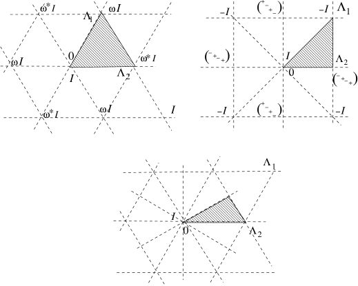
Figure 5: The Stiefel diagrams for $SU(3)$, $Sp(4)$, and $G_{2}$, respectively

The Stiefel diagram of the symplectic group $G=Sp(4)\simeq Spin(5)$ is a right isosceles triangle with vertices $0,\Lambda_{1}$ and $\Lambda_{2}$ (in our labelling conventions, $\alpha_{1}$ is the longest root, so $\Lambda_{1}$ is the longest fundamental weight, corresponding to the five-dimensional representation $SO(5)$; these correspond to the diagonal matrices $I_{4}$, $-I_{4}$, diag$(1,-1,1,-1)$ in $Sp(4)$) (see Figure 5(b)). We can take the maximal torus of $Sp(4)$ to be the diagonal matrices diag$(\xi,\psi,\overline{\xi},\overline{\psi})$ for complex numbers $\xi,\psi$ of modulus 1; then the edges $0\leftrightarrow\Lambda_{1}$, $\Lambda_{1}\leftrightarrow\Lambda_{2}$, $0\leftrightarrow\Lambda_{2}$, respectively, of the Stiefel diagram correspond to the diagonal matrices diag$(\xi,\xi,\overline{\xi},\overline{\xi})$, diag$(\xi,-1,\overline{\xi},-1)$ and diag$(1,\xi,1,\overline{\xi})$. The stabilisers at the vertices are $G$, $G$ and $SU(2)\times SU(2)$ respectively. The stabiliser at the edge $0\leftrightarrow\Lambda_{1}$ is $U(2)$, at the edge $\Lambda_{1}\leftrightarrow\Lambda_{2}$ is $\mathbb{T}\times SU(2)$, and at the edge $0\leftrightarrow\Lambda_{2}$ is $SU(2)\times\mathbb{T}$.

The level-$k$ bundle for $G=SU(2)$ can be constructed as for $T^{r}$, by decomposing a representation of $G$ into weight-spaces (i.e. modules of the maximal torus which are organised by the Weyl group). In particular, let $T$ be the maximal torus consisting of the diagonal matrices – we can naturally identify it with the circle $\mathbb{R}/Q$ where $Q=\sqrt{2}\mathbb{Z}$ is the (co)root lattice. The Hilbert space is ${\mathcal{H}}=L^{2}(G)$. We want to associate a unitary $U_{\gamma}$ to any weight $\gamma\in Q^{*}=1/\sqrt{2}\mathbb{Z}$. To do this, first fix a Stiefel diagram $S$ (here, half of a fundamental domain for $T$). For any subrepresentation $\pi$ in $L^{2}(G)$, define ‘$\pi\otimes\gamma$’ as follows: restrict $\pi$ to $T$ (i.e. write its weight-space decomposition), and in the Weyl-image $wS\subset T$ act like the character $\chi_{w\gamma}(e^{2\pi{\rm i}t})=e^{2\pi{\rm i}\,w\gamma(t)}$. Then thanks to infinite-dimensionality, ${\mathcal{H}}\otimes\gamma\simeq{\mathcal{H}}$ as both a representation of $T$ and the Weyl group, so let $U_{\gamma}$ be the unitary defining that equivalence. We can cover $G\simeq S^{3}$ with two patches: $D_{1}$ about the scalar matrix $I$ and $D_{2}$ about the scalar matrix $-I$. The bundle $\mathcal{A}_{k}$ on $G$ (for $k$ the level), with fibres the compacts $\mathcal{K}=\mathcal{K}({\mathcal{H}})$, is defined by the following gluing condition: identify $(gxg^{-1},c)$ in $D_{1}$ with $(gxg^{-1},Ad(\pi_{g}U_{k}\pi_{g}^{-1})c)$ for any $gxg^{-1}\in D_{1}\cap D_{2}$, $c\in\mathcal{K}$. Again, $U_{k}$ is called the twisting unitary.

The consistency condition for these bundles is that when $gxg^{-1}=x$, then $Ad(\pi_{g}U_{k}\pi_{g}^{-1})$ should be the identity, i.e. $\pi_{g}U_{k}\pi_{g}^{-1}=\lambda_{g}I$ for some character (i.e. one-dimensional representation) $g\mapsto\lambda_{g}$ of the stabiliser $C_{G}(x)$.

When $G=SO(3)$ we have $H^{1}_{G}(G;\mathbb{Z}_{2})\simeq\mathbb{Z}_{2}$ and $H^{3}_{G}(G;\mathbb{Z})\simeq\mathbb{Z}\oplus\mathbb{Z}_{2}$. The representation ring $R_{G}$ is the polynomial ring $\mathbb{Z}[\sigma_{3}]$, while the spinors (corresponding to the torsion part of $H^{3}_{G}$) form the $R_{G}$-module $\sigma_{2}\mathbb{Z}[\sigma_{3}]$. The nontorsion part $\tau_{3,non}\in\mathbb{Z}$ of $H^{3}_{G}$ is done as for $SU(2)$; the torsion part $\tau_{3,tor}$ is done by decomposing the $SO(3)$-module $L^{2}(SU(2))$ into nonspinors (the space for $\tau_{3,tor}=0$) and spinors (for $\tau_{3,tor}=1$). The $H^{1}_{G}$-twist is handled analogously to that of $\mathbb{T}$, by putting a grading on the $SO(3)$-module $L^{2}(SU(2))={\mathcal{H}}_{ns}\oplus{\mathcal{H}}_{sp}$ and using the odd automorphism $U=\left(\begin{matrix}0&a^{\frac{1}{2}}\cr a^{-\frac{1}{2}}&0\end{matrix}\right)$ (where $a^{\frac{1}{2}}\in L^{2}(\widetilde{\mathbb{T}})$ at a generic point) on the overlap.

The level-$k$ bundle for $G=SU(3)$ is similar to that of $SU(2)$. Cover the Stiefel diagram with a patch $D_{0},D_{1},D_{2}$ about each vertex. To the overlap between patch $i$ and patch $j$, assign the twisting unitary $U_{ij}:=U_{k(\Lambda_{j}-\Lambda_{i})}$ (where $\Lambda_{0}:=0$). We must check the consistency condition – it suffices to consider the boundary of the Stiefel diagram, say the edge diag$(z,z,z^{-2})\subset T^{2}$. Which character of the stabiliser $\{{\rm diag}(U),det(U)^{-1})\}\simeq U(2)$ restricts to the character $k\Lambda_{1}$ of the torus $T^{2}$ of $SU(3)$? On that edge the twisting unitary acts like $determinant^{k}$ (the only one-dimensional representations of the stabiliser $U(2)$).

The level-$k$ bundle for $G=Sp(4)$ is the same; the unitary on the edges again corresponds to $det^{k}$. From these examples it should be clear how to obtain any other bundle for $G$ acting adjointly on itself – the $G_{2}$-bundle is explicitly described at the end of section 2.3. Torsion in $H^{3}_{G}$ corresponds to groups $G$ which are nonsimply connected, as we explained with $O(2)$. An $H^{1}_{G}$-twist is obtained by using a double-cover of $G$ to get a grading.

Note that these considerations imply $H^{3}_{G}(G;\mathbb{Z})$ contains $\mathbb{Z}$; of course the former can be calculated by eg. spectral sequences and is found to equal that $\mathbb{Z}$.

For $G$ compact semi-simple (say of rank $r$), Meinrenken [74] found an elegant construction of the $G$ on $G$ bundle at level 1, using the basic representation of the associated affine algebra. Think of the Stiefel diagram as an $r$-dimensional simplex with $r+1$ vertices, labelled say from 0 to $r$. Every nonempty subset $I$ of $\{0,1,\ldots,r\}$ are the vertices of a subsimplex, parametrising points in $G$ containing some stabiliser $G_{I}$ (though the boundary points of this subsimplex will have larger stabiliser). The Lie algebra of $G_{I}$ is naturally identified with the Lie algebra obtained from the affine algebra of $G$, obtained by deleting the vertices $I$ from the affine Dynkin diagram. More precisely, we get a natural embedding of the (finite-dimensional) Lie algebras of these stabilisers, into the (infinite-dimensional) loop algebra. The level 1 basic representation of that affine algebra then restricts to a coherent family of projective representations of those stabilisers, and from this the bundle is formed (see equation (21) in [74]). By using the affine algebra representation, he obtains almost for free a global description of the bundle, avoiding our complicated explicit construction of unitaries and verification of their consistency conditions. On the other hand our construction is more general, permitting eg. $H^{1}_{G}$-twists, is more explicit (which can help in identifying some of the maps in six-term and Mayer-Vietoris sequences), and is inherently finite-dimensional.

In both the physics literature [38, 72] and mathematics literature (this is done very explicitly in [74]), primaries are identified with certain conjugacy classes in $G$. For example, when $G$ is of A-D-E type, the level $k$ primaries are naturally identified with the conjugacy classes corresponding to points in the Stiefel diagram with Dynkin labels $\xi_{i}\in(1/(k+h^{\vee}))\mathbb{Z}$. From our standpoint, a natural task would be to associate to each of these conjugacy classes, a section of the $G$ on $G$ bundle.

This is fairly straightforward to do for $G=\mathbb{T}$ – see the end of section 3.1 for the details for twisted $K$-theory.

2.3 The level calculations

Using the bundles constructed in subsection 2.2, we can compute the level $k$ of the conformal embeddings $H_{k}\rightarrow G_{1}$. This provides a nontrivial consistency check. In this subsection we work out several examples.

Consider first the $\mathbb{T}_{2}\rightarrow SU(2)_{1}$ conformal embedding. The level ‘2’ arises as the inner product $\alpha\cdot\alpha$: as we wrap around $T$, we traverse the Stiefel diagram of $SU(2)$ twice, and so pass through the overlap of the bundle cover, twice. The first time picks up the unitary $U_{\Lambda}$, and the second picks up the unitary $U^{*}_{r.\Lambda}$ where we Weyl reflect the fundamental weight $\Lambda$ (we invert $U$ because the overlap is traversed in the opposite direction). The resulting unitary corresponds to weight $\Lambda-r(\Lambda)=\alpha$, and hence to $T$-character $\alpha\cdot\alpha=2$.

The level $k\in{\rm Hom}(A_{2},A_{2}^{*})$ for $T^{2}_{k}\rightarrow SU(3)_{1}$ ($A_{2}$ is the hexagonal lattice) is recovered very similarly, and this shows how this works in general for conformal embeddings of the maximal torus. For convenience make the patch about the $\Lambda_{2}$-vertex of the $SU(3)$ Stiefel diagram very small, as in Figure 5. This $A_{2}$ (co)root lattice is the span of the simple roots $\alpha_{1},\alpha_{2}$. Move first along the $\alpha_{1}$-direction: we cross from the 0-patch to the $\Lambda_{1}$-patch, given by unitary $U_{r_{\alpha_{2}}(\Lambda_{1})}=U_{\Lambda_{1}}$, and back again, given by $U_{r_{\alpha_{1}}r_{\alpha_{2}}(\Lambda_{1})}^{*}=U_{\Lambda_{1}-\alpha_{1}}^{*}$. As with the $SU(2)$ calculation, $k(\alpha_{1})\in A_{2}^{*}$ will be the net weight picked up, and will equal the difference $\Lambda_{1}-(\Lambda_{1}-\alpha_{1})=\alpha_{1}$. Similarly, $k(\alpha_{2})=\alpha_{2}$, so the $LT^{2}$-level $k$ is given by the identity map.

More interesting is to recover from the bundles the level for the conformal embedding of $SU(2)$ (or more precisely $SO(3)$) into $SU(3)$. This map $\mathcal{R}^{(3)}$ is given explicitly in (5.2) below, from which we read off that the $SU(2)$ Stiefel diagram $I_{2}\leftrightarrow-I_{2}$ embeds into the line $(2t,0,-2t)$ in the $SU(3)$ Cartan subalgebra $(x,y,-x-y)$ as in Figure 6: the endpoints correspond to $t=0$ and $t=\frac{1}{2}$ (the $-I_{2}$-endpoint should lie at the first coroot lattice point on the segment after 0, since $-I_{2}$ lies in the kernel of $\mathcal{R}^{(3)}$). The $SU(2)$ simple root, in this $SU(3)$ notation, corresponds to $t=1$. As we move along this $SU(2)$ Stiefel diagram, we see we twice have to change patches in the $SU(3)$ bundle. As always, this is where the twisting unitaries arise: the net twist here is $\Lambda_{1}-r_{\alpha_{1}+\alpha_{2}}(\Lambda_{1})=\alpha_{1}+\alpha_{2}=(1,0,-1)$. This will correspond to an $SU(2)$ twist of $k\Lambda_{1}^{su2}$ where the level $k$ is obtained by the inner product of the net twist $(1,0,-1)$ with the $SU(2)$ simple root $(2,0,-2)$. In this way we recover the value $k=4$.

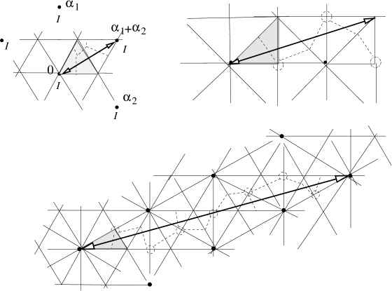
Figure 6: $SU(2)$ Stiefel diagram in $SU(3)$, $Sp(4)$, $G_{2}$ Cartan subalgebras

The conformal embedding of $SU(2)$ into $Sp(4)$, given explicitly by $\mathcal{R}^{(4)}$ in (6.2) below, behaves similarly. The $SU(2)$ Stiefel diagram embeds into the line $\frac{1}{\sqrt{2}}(3t,t)$ in the $Sp(4)$ Cartan subalgebra $(x,y)$ as in Figure 6, with endpoints at $t=0$ and $t=1$; $t=2$ is the $SU(2)$ simple root (here, the simple root should correspond to the first coroot lattice point on the segment after 0, since $-I_{2}$ does not lie in the kernel of $\mathcal{R}^{(4)}$). As we move along this $SU(2)$ Stiefel diagram, we change patches three times, for a net twist of $\frac{1}{\sqrt{2}}(1,1)-\frac{1}{\sqrt{2}}(-1,1)+\frac{1}{\sqrt{2}}(1,1)=\frac{1}{\sqrt{2}}(3,1)$. The level $k$ is thus $\frac{1}{\sqrt{2}}(3,1)\cdot\frac{1}{\sqrt{2}}(6,2)$. In this way we recover the value $k=10$.

The conformal embedding of $SU(2)$ (more precisely, $SO(3)$) into the compact Lie group of type $G_{2}$, can be analysed similarly, except we don’t give the explicit form for it (it will take the form of the 7-dimensional irreducible two-to-one representation of $SU(2)$, embedded into the 7-dimensional irreducible representation of $G_{2}$, whose image can be identified with $G_{2}$). Choosing the realisation roots $\alpha_{1}=(-1,2,-1)/\sqrt{3}$, $\alpha_{2}=(1,-1,0)/\sqrt{3}$, the Stiefel diagram can be taken to be the triangle with vertices at 0, $\Lambda_{2}=(1,0,-1)/\sqrt{3}$ and $\Lambda_{1}/2=(1,1,-2)/2\sqrt{3}$ (with the twisting unitaries in each patch given by the weights $2(\Lambda_{2}-0)$, $2(\Lambda_{1}/2-0)$, $2(\Lambda_{1}/2-\Lambda_{2})$ – the doubling is needed to get $G_{2}$ weights). Because we don’t have the explicit mapping, we need help to see how the $SU(2)$ Stiefel diagram fits inside the $G_{2}$ Cartan subalgebra: Table 13 of [29] tells us the $SU(2)$ Cartan subalgebra is the line $t(10\alpha_{1}+18\alpha_{2})=\frac{t}{\sqrt{3}}(8,2,-10)$ (see Figure 6). The endpoints of the $SU(2)$ Stiefel diagram are thus at $t=0$ and $t=\frac{1}{2}$, and the $SU(2)$ simple root is at $t=1$. We get 8 patch crossings, for a total twist of $2\times\bigl{(}(2,0,-2)-(0,2,-2)+(-2,0,2)+(-1,0,1)\bigr{)}/\sqrt{3}=(-2,-4,6)/\sqrt{3}$. Thus the $SU(2)$ level is $k=(-2,-4,6)\cdot(8,2,-10)/3=-28$.

3 Conformal embeddings: the first examples

Given a conformal embedding $H_{k}\rightarrow G_{\ell}$ and the choice of diagonal $G_{\ell}$ modular invariant ${Z}=\sum_{\mu}|\chi_{\mu}|^{2}$, it is natural to guess that ${}^{\tau}K_{*}^{H}(G)$ recovers the full system of the corresponding $H_{k}$ modular invariant – see the end of section 1.4 for the finite group analog of this statement, which works perfectly. As we will find, this $K$-homological interpretation of conformal embeddings of loop groups isn’t as clean as one would like. We will give in this section the easiest nontrivial examples, and in sections 5 and 6 give more serious examples.

In order for this approach to conformal embeddings to work, we should have that $H^{3}_{H}(G;\mathbb{Z})$ contains a copy of $\mathbb{Z}$ which can be identified with $H^{3}_{G}(G;\mathbb{Z})\,$. But an element of $H^{3}_{G}(G;\mathbb{Z})$ corresponds to a $G$-equivariant bundle $K_{\tau}$ of compact operators on $G$, as explained in section 1.1, so restricting equivariance to $H$ defines the appropriate element of $H_{H}^{3}(G;\mathbb{Z})\,$. This can also be seen from the Borel construction of group cohomology $H^{*}_{G}(X)=H^{*}((X\times EG)/G)\,$: we can identify the universal coverings $EH$ with $EG$, so the natural projection $(X\times EG)/H\rightarrow(X\times EG)/G$ becomes the map $H^{*}_{G}(X)\rightarrow H^{*}_{H}(X)\,$.

3.1 The Verlinde algebras for the circle

We consider here the $K$-homology calculations of the level $k$ Verlinde algebra of the circle $\mathbb{T}$, where this is understood as in section 1.2. This falls under the Freed-Hopkins-Teleman umbrella and constitutes the easiest example.

In fact the calculation is given in section 4 of [43]. Let $L\subset\mathbb{R}^{n}$ be an $n$-dimensional lattice and $L^{*}={\rm Hom}(L,\mathbb{Z})$ be the dual lattice, and consider the $n$-torus $T=\mathbb{R}^{n}/L$. As mentioned earlier, the twist $\tau$ here (the ‘level’) lies in ${\rm Hom}(L,L^{*})$. They obtain ${}^{\tau}K_{0}^{T}(T)\simeq\mathbb{Z}\langle L^{*}/\tau(L)\rangle$, the Verlinde algebra, and ${}^{\tau}K_{1}^{T}(T)=0$.

In order to motivate the calculations given next section, it is helpful to redo this calculation explicitly for the maximal torus $\mathbb{R}/\sqrt{2}\mathbb{Z}$ of $SU(2)$. The orbit analysis is trivial: we have $\mathbb{T}$ acting on itself by conjugation, but because it’s abelian this action is trivial. So each point of $\mathbb{T}$ is itself an orbit, with full stabiliser $\mathbb{T}$. Here, $L=\sqrt{2}\mathbb{Z}$ and $L^{*}=\frac{1}{\sqrt{2}}\mathbb{Z}$, and the twist $\tau$ can be identified with a nonzero even integer $k$ (so $L^{*}/\tau(L)\simeq\mathbb{Z}/k\mathbb{Z}$).

The $K_{*}$-groups are most simply computed by Mayer-Vietoris (1.10):

$$\begin{matrix}{}^{\tau}K^{\mathbb{T}}_{0}(\mathbb{T})&\longrightarrow&K^{\mathbb{T}}_{0}(\mathbb{R})\times 2&\longrightarrow&K^{\mathbb{T}}_{0}(\mathbb{R})\times 2\cr\uparrow&&&&\downarrow\cr K^{\mathbb{T}}_{1}(\mathbb{R})\times 2&{\beta\atop\longleftarrow}&K^{\mathbb{T}}_{1}(\mathbb{R})\times 2&\longleftarrow&{}^{\tau}K^{\mathbb{T}}_{1}(\mathbb{T})\end{matrix}$$ (3.1)

$K_{1}^{\mathbb{T}}(\mathbb{R})$ is the representation ring $R_{\mathbb{T}}=\mathbb{Z}[a^{\pm 1}]$; we’ve dropped the twist on those $K$-homology groups because $H^{1}_{\mathbb{T}}(\mathbb{R};\mathbb{Z}_{2})$ and $H^{3}_{\mathbb{T}}(\mathbb{R};\mathbb{Z})$ both vanish. The map $\beta:R_{\mathbb{T}}{}^{2}\rightarrow R_{\mathbb{T}}{}^{2}$ presumably sends $(p(a),q(a))$ to $(p(a)+q(a),p(a)\pm a^{k}q(a))$, where ‘$k$’ is the $L\mathbb{T}$ level. The effect of the $H^{1}$-twist would be to introduce the sign (‘+’ should correspond to ungraded, in order to recover the nonequivariant $K$-homology $K_{*}(\mathbb{T})=\mathbb{Z}$). Then ${}^{\tau}K^{\mathbb{T}}_{0}(\mathbb{T})={\rm coker}\,\beta=\mathbb{Z}[a^{\pm 1}]/(1\mp a^{k})$ (where we take the lower sign, i.e. ‘+’, if we $H^{1}$-twist) and ${}^{\tau}K^{\mathbb{T}}_{1}(\mathbb{T})={\rm ker}\,\beta=0$. We can also handle the $H^{1}$-twist through (1.7), writing ${}^{\tau}K_{*}^{\mathbb{T}}(\mathbb{T})\simeq{}^{\tau^{\prime}}K_{*+1}^{\mathbb{T}}(M\ddot{o}b)$ where $M\ddot{o}b$ is the open Möbius strip, and $\tau^{\prime}\in H^{3}_{G}(G;\mathbb{Z})$ is the nontorsion part of $\tau$.

Now, $\mathbb{Z}[a^{\pm 1}]/(1-a^{k})$ corresponds to a $k$-dimensional ring with cyclic fusion product generated by $a$. For $k$ odd, $\mathbb{Z}[a^{\pm}]/(1+a^{k})$ is also cyclic, with generator $-a$, but for $k$ even that $k$-dimensional ring is not cyclic. This seems to suggest that we should not $H^{1}$-twist here.

In summary, for this $L\mathbb{T}$ example, $K_{1}$ vanishes and $K_{0}$ gives the Verlinde algebra. We should not $H^{1}$-twist these $K_{*}$-groups.

Using the bundle $\mathcal{A}_{k}$ constructed in subsection 1.2, the six-term exact sequence (1.9) (removing a point from $\mathbb{T}$) becomes

$$\begin{array}[]{ccccc}0&{\longleftarrow}&K^{0}(C_{0}(X;\mathcal{A}_{k})\rtimes G)&{\longleftarrow}&\mathbb{Z}[a^{\pm 1}]\\[3.0pt] \downarrow&&&&\uparrow\beta\\[2.0pt] 0&{\longrightarrow}&K^{1}(C_{0}(X;\mathcal{A}_{k})\rtimes G)&{\longrightarrow}&\mathbb{Z}[a^{\pm 1}]\end{array}$$ (3.2)

where $\beta$ corresponds to multiplying by $1\mp a^{k}$, depending on the sign of the $H^{1}$-twist. This recovers the previous result.

We can give a more precise description of the dual $K^{*}$-groups which are again most simply computed by Mayer-Vietoris (1.10):

$$\begin{matrix}{}^{\tau}K_{\mathbb{T}}^{0}(\mathbb{T})&\longleftarrow&K_{\mathbb{T}}^{0}(\mathbb{R})\times 2&\longleftarrow&K_{\mathbb{T}}^{0}(\mathbb{R})\times 2\cr\downarrow&&&&\uparrow\cr K_{\mathbb{T}}^{1}(\mathbb{R})\times 2&{\gamma\atop\longrightarrow}&K_{\mathbb{T}}^{1}(\mathbb{R})\times 2&\longrightarrow&{}^{\tau}K_{\mathbb{T}}^{1}(\mathbb{T})\end{matrix}$$ (3.3)

To keep track, we call the open sets $U_{1}$ and $U_{2}$ both homeomorphic to $\mathbb{R}$ in $\mathbb{T}$. Regard this as : $\gamma$ is surjective on the first co-ordinate, so $K^{1}_{\mathbb{T}}(U_{1})$ does not contribute to $K^{1}_{\mathbb{T}}(\mathbb{T})$ under the map $\gamma$ – indeed it is killed by $\gamma$. So $K^{1}_{\mathbb{T}}(\mathbb{T})$ is described by $K^{1}_{\mathbb{T}}(U_{2})$ – under $\gamma$. However, because of exactness there are relations imposed on $K^{1}_{T}(U_{2})$ when mapped into $K^{1}_{\mathbb{T}}(\mathbb{T})$, namely

$$K^{1}_{\mathbb{T}}(\mathbb{T})\simeq K^{1}_{\mathbb{T}}(U_{1})/(1-\alpha^{k})K^{1}_{\mathbb{T}}(U_{1})\simeq R_{\mathbb{T}}/(1-\alpha^{k})R_{\mathbb{T}}\,.$$

An alternative viewpoint is via the six-term exact sequence for $K$-theory, for the open set $U=\mathbb{T}$ with a point removed. This gives $K^{1}_{\mathbb{T}}(\mathbb{T})\simeq K^{1}_{\mathbb{T}}(U)/\exp(K^{1}_{\mathbb{T}}(pt))\,$, using the exponential map.

This yields the following description of $K^{1}_{\mathbb{T}}(\mathbb{T})$ in terms of unitaries in the (unitalisation) of the twisted bundle ${\mathcal{A}}_{k}$ of section 2.2 of compacts on the circle. The sections of the bundle are maps $f$ from $[0,1]$ into ${\mathcal{K}}(L^{2}(\mathbb{T}))$ such that $f(0)=Ad(U_{k})(f(1))$, where $U_{k}$ is the unitary associated with the twist $k$. Take the equivariant Bott map $\beta:K^{0}_{\mathbb{T}}(pt)\rightarrow K^{1}_{\mathbb{T}}(U)$ , where $1$ is the unit of $\mathbb{(}T)$ Then $\beta(1)=w_{0}=ze_{0}+1-e_{0}$, where $z$ is the natural loop in $\mathbb{T}$, and $e_{j}$ is the projection in $L^{2}(\mathbb{T})$ corresponding to the character $j$. The action of $\mathbb{Z}_{k}$, identified with the $\{\omega^{j}:j\}$ where $\omega=\exp(2\pi i/k)$ on $\mathbb{T}$ by rotation induces an action on the bundle ${\mathcal{A}}_{k}$ and hence on $K^{1}_{\mathbb{T}}(\mathbb{T})$. (This is best seen by breaking up the bundle into an equivalent one where we have $k$ cuts on the circle with a jump indicated by $U_{1}$ at each, so that sections of the bundle are maps $f$ from $[0,1]$ into ${\mathcal{K}}(L^{2}(\mathbb{T}))$ such that $f(j/k)=Ad(U_{1})(f((j+1)/k))\,,i=0,1,\dots k-1$) This rotation takes the generator $[w_{0}]$ to $[w_{j}]=[ze_{j}+1-e_{j}]$, compatible with the equivariant Bott maps $\beta:K^{0}_{\mathbb{T}}(\omega^{j})\rightarrow K^{1}_{\mathbb{T}}(U)$ . Note that $[w_{n}]=[w_{n+k}]$ in $K^{1}$ due to the nature of the bundle ${\mathcal{A}}_{k}$. The labelling of the $k$ primary fields has a dual meaning in terms of the representations of $\mathbb{T}$ or of the (conjugacy classes) of the points $\{\omega^{j}:j\}$ on the circle.

3.2 The $\mathbb{T}_{2}\rightarrow SU(2)_{1}$ conformal embedding

We consider next the $K$-homology calculations of the conformal embedding $\mathbb{T}_{2}\rightarrow SU(2)_{1}$ (corresponding to ‘$A_{2}$’ on the A-D-E list of modular invariants in [22]). The $\mathbb{T}$ level is most easily obtained by comparing characters: the two irreducible level 1 characters of the loop group $LSU(2)$ are theta functions divided by $\eta(\tau)$, and coincide with the two $L\mathbb{T}_{2}$ characters (so the branching rules here are trivial). This conformal embedding, together with the diagonal $SU(2)_{1}$ modular invariant, yields the diagonal $\mathbb{T}_{2}$ modular invariant ${Z}=I$. The resulting full system should thus be two-dimensional. In fact it should be identifiable with the cyclic Verlinde algebra $\mathbb{Z}[a^{\pm 1}]/(1-a^{2})$.

The orbit analysis is easy: we have the maximal torus $\mathbb{T}$ acting on $SU(2)$ by conjugation, where we identify $\mathbb{T}$ with the diagonal matrices $\left(\begin{matrix}\alpha&0\cr 0&\overline{\alpha}\end{matrix}\right)$. The orbits are ${\mathcal{O}}_{f}=\mathbb{T}$ (the diagonal matrices), with the full $\mathbb{T}$ as stabiliser, and the generic points, with $C_{2}=\pm I$ as stabiliser (corresponding to the centre of $SU(2)$). The generic orbits together form ${\mathcal{O}}_{g}=\mathbb{R}^{2}\times\mathbb{T}/C_{2}$. To see this, parametrise $SU(2)$ with matrices $\left(\begin{matrix}\beta&\gamma\cr-\overline{\gamma}&\overline{\beta}\end{matrix}\right)$ where $|\beta|^{2}+|\gamma|^{2}=1$. The generic orbits correspond to $\gamma\neq 0$; the resulting $\mathbb{T}$ orbit will contain exactly one matrix whose $\gamma$ entry is a positive real number. Hence each generic orbit is uniquely determined by its value of $\beta$, which will lie in the interior of the unit disc, and this is the $\mathbb{R}^{2}$.

Next, we need the cohomology groups $H^{1}_{\mathbb{T}}(\mathbb{T};\mathbb{Z}_{2})=\mathbb{Z}_{2}$, $H^{3}_{\mathbb{T}}(\mathbb{T};\mathbb{Z})=\mathbb{Z}$, $H^{1}_{\mathbb{T}}(\mathbb{R}^{2}\times\mathbb{T}/C_{2};\mathbb{Z}_{2})={\rm Hom}(C_{2},\mathbb{Z}_{2})=\mathbb{Z}_{2}$ and $H^{3}_{\mathbb{T}}(\mathbb{R}^{2}\times\mathbb{T}/C_{2};\mathbb{Z})=0$. $H^{*}_{\mathbb{T}}$ for ${\mathcal{O}}_{f}$ was easiest to compute using Künneth. Also, spectral sequences immaediately tell us $H^{1}_{\mathbb{T}}(SU(2);\mathbb{Z}_{2})=0$ and $H^{3}_{\mathbb{T}}(SU(2);\mathbb{Z})$ is either $\mathbb{Z}$ or 0 (hence we know $H^{3}_{\mathbb{T}}(SU(2);\mathbb{Z})=\mathbb{Z}$, since it must see the level $k$).

The obvious six-term exact sequence reads

$$\begin{matrix}K^{C_{2}}_{1}(pt)&\longleftarrow&{}^{\tau}K^{\mathbb{T}}_{0}(SU(2))&\longleftarrow&{}^{\tau^{\prime\prime}}K^{\mathbb{T}}_{0}(\mathbb{T})\cr\downarrow&&&&\uparrow\beta\cr{}^{\tau^{\prime\prime}}K^{\mathbb{T}}_{1}(\mathbb{T})&\longrightarrow&{}^{\tau}K^{\mathbb{T}}_{1}(SU(2))&\longrightarrow&K^{C_{2}}_{0}(pt)\end{matrix}$$ (3.4)

The $K_{*}$-groups for orbits ${\mathcal{O}}_{f}$ are computed last subsection, and we obtain ${}^{\tau^{\prime}}\!K^{\mathbb{T}}_{0}(\mathbb{T})=\mathbb{Z}[a^{\pm 1}]/(1-a^{2(k+2)})\simeq\mathbb{Z}^{2(k+2)}$ and ${}^{\tau^{\prime}}K^{\mathbb{T}}_{1}(\mathbb{T})=0$ (since there is no $H^{1}$-twist here). Here, $a$ is the generator of the representation ring $R_{\mathbb{T}}$, and $k+2$ is the $LSU(2)$ level shifted as usual by its dual Coxeter number ($k=1$ corresponds to the conformal embedding). The factor there of 2 is explained in subsection 2.3. Also, $K_{0}^{C_{2}}(pt)=R_{C_{2}}\simeq\mathbb{Z}^{2}$ and $K_{1}^{C_{2}}(pt)=0$, and $\beta$ is an injection. We obtain $K_{0}^{\mathbb{T}}(SU(2))\simeq\mathbb{Z}^{2k+2}$ and $K_{1}^{\mathbb{T}}(SU(2))=0$. (We compute this more elegantly in the following subsection. This example was also computed in [93].)

Again, $k=1$ corresponds to the conformal embedding, but its full system is only two-dimensional, not four. Next subsection we find that a similar phenomenon occurs with many other conformal embeddings. There we identify the multiplicity two occurring here with the order of the Weyl group $C_{2}$ of $SU(2)$, or if you prefer with the Euler number of the sphere $SU(2)/\mathbb{T}$. We discuss what this could mean in the concluding section.

3.3 The Hodgkin spectral sequence

The Hodgkin spectral sequence (Thm. 6.1 of [91]) is a powerful tool for calculating many $K$-groups ${}^{\tau}K_{H}^{*}(G)$. In particular, suppose $G$ is a compact connected Lie group, with torsion-free fundamental group (eg. a torus $T^{n}$ or a simply connected group), and $H$ is a closed subgroup of $G$. As in section 1.1, let $X$ be a space on which $G$ acts, so $B=C_{0}(X;\mathcal{K}_{\tau})$ is a $C^{*}$-algebra carrying a $G$-action. Then there is a spectral sequence of $R_{G}$-modules which strongly converges to $K_{*}^{H}(B)={}^{\tau}K_{H}^{*}(X)$, with

$$E^{2}_{p,q}={\rm Tor}_{p}^{R_{{G}}}(R_{H},{}^{\tau}K^{q}_{G}(X))\,.$$ (3.5)

We are most interested in $X=G$, with the adjoint action of $G$, in which case ${}^{\tau}K^{q}_{G}(X)=Ver_{k}(G)$ or 0, for a level $k$ determined from $\tau$.

Consider first the situation where $H$ is maximal (i.e. of full rank) in $G$. There are many examples of this, eg. $SU(n)_{1}\rightarrow SU(p)_{1}\times SU(n-p)_{1}\times U(1)_{np(n-p)}$, $G_{2,1}\rightarrow SU(2)_{3}\times SU(2)_{1}\,$, $E_{8,1}\rightarrow SU(9)_{1}$ are some among infinitely many ([94] used essentially this method to compute a subset of these, namely those corresponding to Hermitian symmetric spaces). When $H$ is of maximal rank, [86] (together with the validity of Serre’s conjecture that projective modules over polynomial rings over fields or PIDs are free) tells us that $R_{H}$ is free over $R_{G}$, say $R_{H}\simeq(R_{G})^{d}$. This means that $E^{2}_{0,q}=Ver_{1}(G)\otimes_{R_{G}}R_{H}$ for $q$ odd, and all other $E^{2}_{p,q}$ vanish. Hence ${}^{\tau}K^{0}_{H}(G)=0$ and

$${}^{\tau}K^{1}_{H}(G)=Ver_{1}(G)\otimes_{R_{G}}R_{H}=R_{H}/{I}_{1}=(Ver_{1}(G))^{d}\,,$$ (3.6)

where ${I}_{1}$ is the level-1 fusion ideal given by $Ver_{1}(G)\simeq R_{G}/\mathcal{I}_{1}\,$. This rank $d$ is given by $d=|W_{G}|/|W_{H}|\,$, the Euler number of $G/H$, where $W_{G},W_{H}$ are the Weyl groups of $G,H$ respectively (see equation (2.9) of [94] for the easy derivation).

One of the easiest of these examples is $E_{8,1}\rightarrow SU(9)_{1}\,$: there is only one $E_{8,1}$ modular invariant, namely the diagonal one, and it restricts to the $SU(9)_{1}$ modular invariant ${Z}=|\chi_{00000000}+\chi_{00100000}+\chi_{00000100}|^{2}$. The full system of ${Z}$ will be 9-dimensional. On the other hand $Ver_{1}(E_{8})$ is 1-dimensional, and $|W_{E8}|/|W_{SU9}|=1920$, so ${}^{\tau}K^{1}_{SU9}(E_{8})$ is 1920-dimensional. There certainly is room in ${}^{\tau}K^{1}_{SU9}(E_{8})$ for the full system, but the meaning of the rest is unclear to us, and again is discussed in section 7.

For most conformal embeddings, $H$ does not have full rank, but at least when $G$ has small rank, then this spectral sequence can still be very useful. We will see this in section 6.1 below, where we compute ${}^{\tau}K_{H}^{*}(G)$ for $SU(2)_{10}\rightarrow Sp(4)_{1}$. Unfortunately, for the embedding $SU(2)_{4}\rightarrow SU(3)_{1}$ considered in section 5 (similarly $SU(2)_{28}\rightarrow G_{2,1}$), it is the homomorphic image $SO(3)$ and not $SU(2)$ which is embedded in $SU(3)$, while we are interested in the $K$-groups with respect to $SU(2)$. For those examples, the Hodgkin spectral sequence does not seem to have a direct use and we must dive into the orbit analysis.

4 Permutation orbifolds

Let $G$ be connected compact and simply connected (although we also take $G=\mathbb{T}$ below), and let $\pi$ be any subgroup of the symmetric group $S_{n}$. Over $\mathbb{C}$, the corresponding orbifold by $\pi$ of $n$ copies of $G$ on $G$, will be given by the centre of the crossed-product construction $({}^{\tau}K_{0}^{G^{n}}(G^{n})){\times\!\vrule height=5.0pt,depth=0.0pt,width=0.4pt\,}\pi=K^{0}(C(G^{n};\mathcal{K}_{\tau})\otimes C^{*}(G^{n})){\times\!\vrule height=5.0pt,depth=0.0pt,width=0.4pt\,}\pi$, where $G^{n}$ acts adjointly on $G^{n}$ in the obvious way, and $\pi$ acts by permuting these $n$ factors. It is tempting to approximate this geometrically, by guessing that the Verlinde algebra of this $\pi$-permutation orbifold of $G$ is ${}^{\tau}K_{*}^{G^{n}{\times\!\vrule height=5.0pt,depth=0.0pt,width=0.4pt\,}\pi}(G^{n})$, where $*=0$ and $G^{n}$ acts adjointly on $G^{n}$ while $\pi$ acts on the space $G^{n}$ by permuting. We need the semi-direct product $G^{n}{\times\!\vrule height=5.0pt,depth=0.0pt,width=0.4pt\,}\pi$ of groups, rather than direct product, for this to be a group action ($\pi$ will likewise act on the subgroup $G^{n}$ by permuting). For $*=1$, we’d expect a trivial $K$-homology group.

For this idea to work, we would expect that $H^{3}_{G^{n}{\times\!\vrule height=5.0pt,depth=0.0pt,width=0.4pt\,}\pi}(G^{n};\mathbb{Z})$ contains a $\mathbb{Z}$ which can be identified with $H^{3}_{G}(G;\mathbb{Z})$. This can be seen as follows. An element of $H^{3}_{G}(G;\mathbb{Z})$ corresponds to a $G$-equivariant bundle $K_{\tau}$ of compacts on $G$. Taking the product of $n$ of these bundles, we have a $G^{n}$ bundle of compacts on $G^{n}$. For this to make sense under the action of the permutation group $\pi$, we require choosing the same bundle (i.e. one element of $H_{G}^{3}(G;\mathbb{Z})$) $n$ times. This gives a map from $H^{3}_{G}(G;\mathbb{Z})$ to $H^{3}_{G^{n}{\times\!\vrule height=5.0pt,depth=0.0pt,width=0.4pt\,}\pi}(G^{n};\mathbb{Z})$, which shouldn’t be the zero map. In section 4.2 we generalise slightly this construction, owing to an extra large cohomology group.

To see that this is not unreasonable, consider the $\mathbb{Z}_{2}$-permutation orbifold of the quantum double of finite abelian groups. Let $G$ be a finite abelian group, of order $n$ say, write $H=(G\times G){\times\!\vrule height=5.0pt,depth=0.0pt,width=0.4pt\,}\mathbb{Z}_{2}\,$, and take trivial twist $\sigma\in H^{4}(BG;\mathbb{Z})\,$. Then $K_{1}^{H}(G\times G)$ is readily seen to vanish, and $K_{0}^{H}(G\times G)$ can be computed by writing the finite set $G\times G$ as the union of the diagonal elements $D=\{(g,g)\}$ and the off-diagonal, the latter parametrised by a set $F$ of $(n^{2}-n)/2$ $\mathbb{Z}_{2}$-orbit representatives $(g,h)$. Then $K_{0}^{H}(D)$ is $\|D\|=n$ copies of $K_{0}^{H}(pt)=R_{H}$, which has dimension $2n+(n^{2}-n)/2$ (the type ${2\atop 1}$- resp. ${1\atop 2}$-representations, using terminology of section 2.1). Also, $K_{0}^{H}(F\times H/(G\times G))$ consists of $\|F\|$ copies of $K_{0}^{G\times G}(pt)=R_{G\times G}\,$, which has dimension $n^{2}$. Thus $K_{0}^{H}(G\times G)$ has dimension $n(n^{2}+n)/2+(n^{2}-n)n^{2}/2=(n^{4}+n^{2})/2\,$, which matches exactly the number of primaries in the $\mathbb{Z}_{2}$-permutation orbifold of the quantum double of $G$. The only curious aspect of this calculation is that $(n^{3}+n^{2})/2$ dimensions are associated to the diagonal $D$, whereas $2n^{2}$ primaries in the orbifold result from the doubling of the $n^{2}$ fixed points. This means the $n^{2}$ fixed point primaries of $\mathcal{D}(G)$ should not be identified with the $n^{2}$ diagonal elements of the ‘space’ $G\times G$, but this should be clear since they are parametrised differently.

We further test this with the $S_{2}$-permutation orbifold of both $\mathbb{T}$ and $SU(2)$.

4.1 The Verlinde algebra of the 2-torus

Before computing the $S_{2}$-permutation orbifold of the circle $\mathbb{T}$, it is convenient to compute the Verlinde algebra of $T^{2}$ explicitly by $K$-homology. (The result for the loop group of any torus is quoted in section 3.1.) Being abelian, the torus $T^{2}=(\mathbb{R}/\sqrt{2}\mathbb{Z})^{2}$ acts trivially on itself. The level here can be any matrix $K=\left(\begin{matrix}k&l\cr m&n\end{matrix}\right)$ with $det\,K\neq 0$. Judging from section 3.1, there should be no $H^{1}$-twist.

Let $\Delta$ be the diagonal $(x,x)$ in the torus $T^{2}$. The six-term sequence will involve the $K$-holomogy of the circle $\Delta$ and the cylinder $T^{2}\setminus\Delta=\mathbb{R}\times\mathbb{T}$, and we will first compute these from Mayer-Vietoris:

$$\begin{array}[]{ccccc}{}^{\tau^{\prime\prime}}K^{T^{2}}_{0}(\Delta)&{\longrightarrow}&0&{\longrightarrow}&0\\[3.0pt] \uparrow&&&&\downarrow\\[2.0pt] 2\times K^{T^{2}}_{1}(\mathbb{R})&\stackrel{{\scriptstyle\alpha\,}}{{\longleftarrow}}&2\times K^{T^{2}}_{1}(\mathbb{R})&{\longleftarrow}&{}^{\tau^{\prime\prime}}K^{T^{2}}_{1}(\Delta)\end{array}$$ (4.1)

$$\begin{array}[]{ccccc}{}^{\tau^{\prime}}K^{T^{2}}_{0}(\mathbb{R}\times\mathbb{T})&{\longrightarrow}&2\times K^{T^{2}}_{0}(\mathbb{R}^{2})&\stackrel{{\scriptstyle\beta\,}}{{\longrightarrow}}&2\times K^{T^{2}}_{0}(\mathbb{R}^{2})\\[3.0pt] \uparrow&&&&\downarrow\\[2.0pt] 0&{\longleftarrow}&0&{\longleftarrow}&{}^{\tau^{\prime}}K^{T^{2}}_{1}(\mathbb{R}\times\mathbb{T})\end{array}$$ (4.2)

Now, $K^{T^{2}}_{0}(\mathbb{R}^{2})=K^{T^{2}}_{1}(\mathbb{R})=R_{T^{2}}=\mathbb{Z}[a^{\pm 1},b^{\pm 1}]$. The map $\alpha$ sends the Laurent polynomials $(p(a,b),q(a,b))$ to $(p+q,p+a^{k+l}b^{m+n}q)$, and so we obtain ${}^{\tau^{\prime\prime}}K_{0}^{T^{2}}(\Delta)=\mathbb{Z}[a^{\pm 1},b^{\pm 1}]/(1-a^{k+l}b^{m+n})$ and ${}^{\tau^{\prime\prime}}K_{1}^{T^{2}}(\Delta)=0$. Similarly, the map $\beta$ sends $(p(a,b),q(a,b))$ to $(p+q,p+a^{k+l}b^{m+n}q)$ (it involves the same cycle on $T^{2}$), and so we obtain ${}^{\tau^{\prime}}K_{1}^{T^{2}}(\mathbb{R}\times\mathbb{T})=\mathbb{Z}[a^{\pm 1},b^{\pm 1}]/(1-a^{k+l}b^{m+n})$ and ${}^{\tau^{\prime}}K_{0}^{T^{2}}(\mathbb{R}\times\mathbb{T})=0$.

Thus, the six-term sequence becomes

$$\begin{array}[]{ccccc}0&{\longleftarrow}&{}^{K}K^{T^{2}}_{0}(T^{2})&{\longleftarrow}&\mathbb{Z}[a^{\pm 1},b^{\pm 1}]/(1-a^{k+l}b^{m+n})\\[3.0pt] \downarrow&&&&\uparrow\ \gamma\\[2.0pt] 0&{\longrightarrow}&{}^{K}K^{T^{2}}_{1}(T^{2})&{\longrightarrow}&\mathbb{Z}[a^{\pm 1},b^{\pm 1}]/(1-a^{k+l}b^{m+n})\end{array}$$ (4.3)

where $\gamma([r(a,b)])=[(1-a^{k}b^{m})r]$. This gives ${}^{K}K^{T^{2}}_{1}(T^{2})=0$ and ${}^{K}K^{T^{2}}_{0}(T^{2})=\mathbb{Z}[a^{\pm 1},b^{\pm 1}]/(1-a^{k+l}b^{m+n},1-a^{k}b^{m})\,$, which as an additive group is isomorphic to the group ring of $\mathbb{Z}^{2}/{\rm Span}\{\left(\begin{matrix}k+l\cr m+n\end{matrix}\right),\left(\begin{matrix}k\cr m\end{matrix}\right)\}\,$. This is in agreement with Theorem 4.2(i) of [43].

4.2 The $S_{2}$-permutation orbifold of the circle

Consider for simplicity the $S_{2}$-permutation orbifold of $\mathbb{T}$ at level $k$. Over $\mathbb{C}$, this will be given by the centre of the crossed-product construction $({}^{\tau}K_{0}^{\mathbb{T}\times\mathbb{T}}(\mathbb{T}\times\mathbb{T})){\times\!\vrule height=5.0pt,depth=0.0pt,width=0.4pt\,}S_{2}=K^{0}(C(\mathbb{T}^{2};\mathcal{K}_{\tau})\otimes C^{*}(\mathbb{T}^{2})){\times\!\vrule height=5.0pt,depth=0.0pt,width=0.4pt\,}S_{2}$. As mentioned above, this suggests the geometric approximation $K^{0}(C(\mathbb{T}^{2};\mathcal{K}_{\tau})\otimes C^{*}(\mathbb{T}^{2}){\times\!\vrule height=5.0pt,depth=0.0pt,width=0.4pt\,}S_{2})={}^{\tau}K_{0}^{\mathbb{T}^{2}{\times\!\vrule height=5.0pt,depth=0.0pt,width=0.4pt\,}S_{2}}(\mathbb{T}^{2})$.

Let $U=T^{2}{\times\!\vrule height=5.0pt,depth=0.0pt,width=0.4pt\,}S_{2}$. We will mimic as much as possible the previous calculation. There are only two orbits: the diagonal circle $\Delta=\{(x,x)\}$, which is fixed by all of $U$; the off-diagonal is the cylinder $(x,\theta)$ with free $S_{2}$-action $(x,\theta)\mapsto(-x,\theta+\pi)$. The level $K$ here should commute with $S_{2}$, i.e. $K=\left(\begin{matrix}k&l\cr l&k\end{matrix}\right)$. Again, $K$ should be invertible, i.e. $|k|\neq|l|$. From the bundle picture, it is clear this gives an element of $H^{3}_{U}(T^{2};\mathbb{Z})$. Strictly speaking, the permutation orbifold of $\mathbb{T}_{k}$ would require taking $l=0$; nonzero $l$ would correspond to a $S_{2}$-orbifold of $T^{2}$ level $K$.

The $K$-homology of $\Delta$ can be computed from Mayer-Vietoris:

$$\begin{array}[]{ccccc}{}^{\tau^{\prime\prime}}K^{U}_{0}(\Delta)&{\longrightarrow}&0&{\longrightarrow}&0\\[3.0pt] \uparrow&&&&\downarrow\\[2.0pt] 2\times K^{U}_{1}(\mathbb{R})&\stackrel{{\scriptstyle\alpha^{\prime}\,}}{{\longleftarrow}}&2\times K^{U}_{1}(\mathbb{R})&{\longleftarrow}&{}^{\tau^{\prime\prime}}K^{U}_{1}(\Delta)\end{array}$$ (4.4)

Now, $K^{T^{2}}_{0}(\mathbb{R}^{2})=R_{T^{2}}=\mathbb{Z}[a^{\pm 1},b^{\pm 1}]$, while $K^{U}_{0}(\mathbb{R})=K^{T^{2}}_{1}(\mathbb{R}^{2})=0$. The representation ring of a double-cover such as $U$, together with its induction and restriction maps, is described in section 2.1:

$$K^{U}_{1}(\mathbb{R})=R_{U}=\mathbb{Z}[\mu_{\Delta}^{\pm 1},\mu,\delta]/(\delta^{2}=1,\delta\mu=\mu)=\mathbb{Z}[\mu_{ij}=\mu_{ji},\delta\mu_{ii}]\,,$$ (4.5)

where $\mu_{10}=\mu$, $\mu_{\Delta}=\mu_{11}$, and $\mu_{ij}\mu_{\Delta}^{k}=\mu_{i+k,j+k}$. Induction from $T^{2}$ to $U$ takes both $a^{i}b^{j}$ and $a^{j}b^{i}$ (for $i\neq j$) to the two-dimensional irreducible representation $\mu_{ij}$, and it takes the $S_{2}$-fixed point $a^{n}b^{n}$ to $\mu_{nn}+\delta\mu_{nn}$ ($S_{2}$ acts on $R_{T^{2}}$ by interchanging $a$ and $b$). The map $\alpha^{\prime}$ sends the polynomials $(p(\mu_{\Delta},\mu,\delta),q(\mu_{\Delta},\mu,\delta))$ to $(p+q,p+\mu_{\Delta}^{k+l}q)$, and so we obtain ${}^{\tau^{\prime\prime}}K_{0}^{U}(\Delta)=R_{U}/(1-\mu_{\Delta}^{k+l})$ and ${}^{\tau^{\prime\prime}}K_{1}^{U}(\Delta)=0$.

The $K$-homology of the cylinder $cyl=T^{2}\setminus\Delta$ is more difficult. Write ${}^{\tau}K_{*}^{U}(cyl)=K^{*}_{S_{2}}(C(cyl;\mathcal{K}_{\tau})\otimes C^{*}(T^{2}))$ (which we can do because $T^{2}$ is normal in $U$), and split these representations $C^{*}(T^{2})\simeq C_{0}(\mathbb{Z}^{2})$ into the $S_{2}$-fixed points $C_{0}(\mathbb{Z})$ (the diagonal) and $C_{0}(\mathbb{Z}^{2}\setminus\mathbb{Z})$ (the upper and lower triangles). Because $S_{2}$ fixes that diagonal, we may write $K^{*}_{S_{2}}(C(cyl)\otimes C_{0}(\mathbb{Z}))={}^{k+l}K_{*}^{\mathbb{T}\times S_{2}}(cyl)$, and because $S_{2}$ is normal in $\mathbb{T}\times S_{2}$ and acts freely on $cyl$, ${}^{\tau}K^{*}_{\mathbb{T}{\times\!\vrule height=5.0pt,depth=0.0pt,width=0.4pt\,}S_{2}}(cyl)\simeq{}^{\tau^{\prime\prime}}K_{\mathbb{T}}^{*}(cyl/S_{2})$ (see (1.15)). But $cyl/S_{2}$ is the open Möbius strip $M\ddot{o}b$. Hence Mayer-Vietoris gives us:

$$\begin{array}[]{ccccc}{}^{\tau^{\prime}}K^{\mathbb{T}}_{0}(M\ddot{o}b)&{\longrightarrow}&2\times K^{\mathbb{T}}_{0}(\mathbb{R}^{2})&\stackrel{{\scriptstyle\beta^{\prime}\,}}{{\longrightarrow}}&2\times K^{\mathbb{T}}_{0}(\mathbb{R}^{2})\\[3.0pt] \uparrow&&&&\downarrow\\[2.0pt] 0&{\longleftarrow}&0&{\longleftarrow}&{}^{\tau^{\prime}}K^{\mathbb{T}}_{1}(M\ddot{o}b)\end{array}$$ (4.6)

The map $\beta^{\prime}$ sends $(P(a),Q(a))$ to $(P+Q,P-a^{k+l}Q)$ (the minus sign comes from the topology of $M\ddot{o}b$), and so we obtain ${}^{\tau^{\prime}}K_{1}^{\mathbb{T}}(M\ddot{o}b)=\mathbb{Z}[a^{\pm 1}]/(1+a^{k+l})$ and ${}^{\tau^{\prime}}K_{0}^{\mathbb{T}}(M\ddot{o}b)=0$.

For the remaining ‘off-diagonal’ part of $C^{*}(T^{2})$, the freeness of this $S_{2}$-action identifies $K^{*}_{S_{2}}(C(cyl;\mathcal{K}_{\tau})\otimes C_{0}(\mathbb{Z}^{2}\setminus\mathbb{Z}))$ with $K^{*}(C(cyl;\mathcal{K}_{\tau})\otimes C_{0}(tri))$, where ‘$tri$’ denotes (say) the lower triangle $\{(m,n)\in\mathbb{Z}^{2}\,|\,m>n\}$. Mayer-Vietoris applied to the cylinder then gives us

$$\begin{array}[]{ccccc}K^{0}(C(cyl)\otimes C_{0}(tri))&{\longrightarrow}&2\times K^{0}(C(\mathbb{R}^{2})\otimes C_{0}(tri))&\stackrel{{\scriptstyle\beta^{\prime\prime}\,}}{{\longrightarrow}}&2\times K^{0}(C(\mathbb{R}^{2})\otimes C_{0}(tri))\\[3.0pt] \uparrow&&&&\downarrow\\[2.0pt] 0&{\longleftarrow}&0&{\longleftarrow}&K^{1}(C(cyl)\otimes C_{0}(tri))\end{array}$$ (4.7)

As usual, the twist on $cyl$ can be trivialised on the open subsets $\mathbb{R}^{2}$, so $K^{0}(C(\mathbb{R}^{2})\otimes C_{0}(tri))$ is the off-diagonal part $\mu R_{U}$ of $R_{U}$. The map $\beta^{\prime\prime}$ sends $(p,q)\in\mu R_{U}\oplus\mu R_{U}$ to $(p+q,p+\mu_{\Delta}^{k+l}q)$, by analogy with section 4.1. Therefore we find $K^{0}(C(cyl;\mathcal{K}_{\tau})\otimes C_{0}(tri))={\rm ker}\,\beta^{\prime\prime}=0$ and $K^{1}(C(cyl;\mathcal{K}_{\tau})\otimes C_{0}(tri))={\rm coker}\,\beta^{\prime\prime}=\mu R_{U}/(1-\mu_{\Delta}^{k+l})$.

The six-term sequence then tells us how to obtain ${}^{\tau}K_{*}^{U}(cyl)$:

$$\begin{array}[]{ccccc}0&{\longleftarrow}&{}^{\tau}K^{U}_{0}(cyl)&{\longleftarrow}&0\\[3.0pt] \downarrow&&&&\uparrow\\[2.0pt] \mathbb{Z}[\mu_{\Delta}^{\pm 1}]/(1-\mu_{\Delta}^{k+l})&{\longrightarrow}&{}^{\tau}K^{U}_{1}(cyl)&{\longrightarrow}&\mu R_{U}/(1-\mu_{\Delta}^{k+l})\end{array}$$ (4.8)

Hence ${}^{\tau}K^{U}_{0}(cyl)=0$ and ${}^{\tau}K^{U}_{1}(cyl)=\mathbb{Z}[\mu_{\Delta}^{\pm 1}]/(1-\mu_{\Delta}^{k+l})\oplus\mu R_{U}/(1-\mu_{\Delta}^{k+l})$, where the left summand is the submodule and the right one is its quotient into $K_{1}$.

Finally, we again use the six-term to compute the desired $K$-homology:

$$\begin{array}[]{ccccc}0&{\longleftarrow}&{}^{\tau}K^{U}_{0}(T^{2})&{\longleftarrow}&R_{U}/(1-\mu_{\Delta}^{k+l})\\[3.0pt] \downarrow&&&&\uparrow\ \gamma^{\prime}\\[2.0pt] 0&{\longrightarrow}&{}^{\tau}K^{U}_{1}(T^{2})&{\longrightarrow}&\mathbb{Z}[\mu_{\Delta}^{\pm 1}]/(1-\mu_{\Delta}^{k+l})\oplus\mu R_{U}/(1-\mu_{\Delta}^{k+l})\mu R_{U}\end{array}$$ (4.9)

The map $\gamma^{\prime}$ first projects ${}^{\tau}K_{1}^{U}(cyl)$ to $\mu R_{U}/(1-\mu_{\Delta}^{k+l})$, killing the submodule $\mathbb{Z}[\mu_{\Delta}^{\pm 1}]/(1-\mu_{\Delta}^{k+l})$, and then (by analogy with section 4.1) multiplies $p\in\mu R_{U}$ by $(1-\mu_{k-l}\mu_{\Delta}^{l})$, since $\mu_{k-l}\mu_{\Delta}^{l}=\,$D-Ind${}_{T^{2}}^{U}a^{k}b^{l}$. Thus we obtain the final answer:

$${}^{\tau}K^{{U}}_{0}(T^{2}) = \,R_{U}/(1-\mu_{\Delta}^{k+l},\mu(1-\mu_{k-l}\mu_{\Delta}^{l}))\,,$$ (4.10)

$${}^{\tau}K^{{U}}_{1}(T^{2}) = \,\mathbb{Z}[\mu_{\Delta}^{\pm 1}]/(1+\mu_{\Delta}^{k+l})\,.$$ (4.11)

Consider for simplicity $l=0$; then this $K$-homology does not quite recover the permutation orbifold of the circle at level $k$. In particular, RCFT tells us that the $k$ diagonal points $(a,a)$, being fixed by $S_{2}$, should get doubled, while $(a,b)$ and $(b,a)$ for $a\neq b$ should be identified. We discuss this further in section 7.

4.3 The $S_{2}$-permutation orbifold of $SU(2)$

Now let $G=SU(2)$, $\mathbb{T}$ be the diagonal matrices, $H=(G\times G){\times\!\vrule height=5.0pt,depth=0.0pt,width=0.4pt\,}\mathbb{Z}_{2}$, and $U=(\mathbb{T}\times\mathbb{T}){\times\!\vrule height=5.0pt,depth=0.0pt,width=0.4pt\,}\mathbb{Z}_{2}$ as before, where $\mathbb{Z}_{2}$ acts on $G\times G$ and $\mathbb{T}\times\mathbb{T}$ by permuting. The orbit analysis for $H$ on $G\times G$ is reminiscent of that of $G$ on $G$ given at the beginning of section 1.4. The poles $(\pm I,\pm I)\in G\times G$ form three $H$-orbits: $\mathcal{O}_{H}=(I,I)\cup(-I,-I)$ is fixed by everything, while $\mathcal{O}_{G\times G}=(I,-I)\cup(-I,I)=H/(G\times G)$ has stabiliser $G\times G$. Let $gen=SU(2)\setminus\{\pm I\}=\mathbb{R}\times G/\mathbb{T}$ be the generic points in $G$; then the orbits $\mathcal{O}_{G\times\mathbb{T}}=\pm I\times gen\cup gen\times\pm I=2\times\mathbb{R}\times H/(G\times\mathbb{T})$ have stabiliser $G\times\mathbb{T}$. The points $(x,y)\in gen\times gen$ are of two kinds: those with $x,y$ conjugate form the orbits $\mathcal{O}_{U}=\mathbb{R}\times H/U$, while the remainder form $\mathcal{O}_{T^{2}}=\mathbb{R}^{2}\times H/T^{2}$. Figure 7 gives the resulting picture.

Figure 7: Figure 7: The orbits of $H$ on $G\times G$

Using the method of section 2.1, we easily find that the irreducible $H$-representations are $\rho_{ij}=\rho_{ji}$ ($i,j\geq 0$), $D$, and $D\rho_{ii}$, where $1=\rho_{00}$ and $D$ are one-dimensional, and these obey $D^{2}=1$ and $D\rho_{ij}=\rho_{ij}$ for $i\neq j$. The induction Ind${}_{G\times G}^{H}(\sigma_{i}\sigma^{\prime}_{j})$ equals $\rho_{ij}=\rho_{ji}$ for $i\neq j$, and $\rho_{ii}+D\rho_{ii}$ otherwise. Analogous comments for the $U$-representations were discussed last subsection. We will shortly need the Dirac inductions D-Ind${}_{G\times\mathbb{T}}^{H}={\rm Ind}_{G\times G}^{H}\circ\,$D-Ind${}_{G\times\mathbb{T}}^{G\times G}$ (see section 2.1 for D-Ind${}_{\mathbb{T}}^{G}$), and D-Ind${}_{U}^{H}$. The latter sends $\mu_{\Delta}^{j}$ (resp. $\delta\mu_{\Delta}^{j}$) to $\rho_{|j|-1,|j|-1}$ (resp. $D\rho_{|j|-1,|j|-1}$) provided $j\neq 0$, and kills both $1$ and $\delta$; it sends $\mu_{ij}$ for $i\neq j$ to $sgn(ij)\,\rho_{|i|-1,|j|-1}$, unless $i=-j$ in which case it yields $-\rho_{|i|-1,|i|-1}(1+D)$.

Let $k$ be the (unshifted) level of $SU(2)$, and $\tau$ the corresponding element of $H_{H}^{3}(G\times G;\mathbb{Z})$, as explained in the second paragraph of section 4. The twist won’t survive on any of these orbit spaces, so their $K$-homology groups can be simply written down: the nonzero ones are $K^{H}_{0}(\mathcal{O}_{H})=2\times R_{H}$, $K^{H}_{0}(\mathcal{O}_{G\times G})=R_{G\times G}$, $K_{1}^{H}(\mathcal{O}_{G\times\mathbb{T}})=2\times R_{G}\otimes R_{\mathbb{T}}$, $K_{1}^{H}(\mathcal{O}_{U})=R_{U}$, and $K_{0}^{H}(\mathcal{O}_{T^{2}})=R_{T^{2}}=\mathbb{Z}[a^{\pm 1},b^{\pm 1}]$.

First we use the six-term sequence to glue the compact set $\mathcal{O}_{H}\cup\mathcal{O}_{G\times G}$ to $\mathcal{O}_{G\times T}\cup\mathcal{O}_{U}$:

$$\begin{array}[]{ccccc}0&{\longleftarrow}&{}^{\tau}K^{H}_{0}(\mathcal{O}_{T^{2}}^{c})&{\longleftarrow}&2\times R_{H}\oplus R_{G\times G}\\[3.0pt] \downarrow&&&&\uparrow\ \alpha\\[2.0pt] 0&{\longrightarrow}&{}^{\tau}K^{H}_{1}(\mathcal{O}_{T^{2}}^{c})&{\longrightarrow}&2\times R_{G\times\mathbb{T}}\oplus R_{U}\end{array}\ ,$$ (4.12)

where $\alpha:R_{G\times\mathbb{T}}\oplus R_{G\times\mathbb{T}}\oplus R_{U}\rightarrow R_{H}\oplus R_{H}\oplus R_{G\times G}$ is given by $\alpha(p_{1},p_{2},q)=\,$D-Ind$(q+b^{k}p_{1},-\mu_{\Delta}^{2k}q+p_{2},p_{1}+b^{k}p_{2})$. The sign in front of the $\mu_{\Delta}$ comes from considering orientations of the edges; the powers $k$ or $2k$ are clear from the bundle picture, where traversing an edge crosses patches in the bundle once or twice respectively.

A tedious but straightforward calculation shows that

$${}^{\tau}K_{0}^{H}(\mathcal{O}_{T^{2}}^{c}) = \mathrm{coker}\,\alpha=R_{H}/(\rho_{ij}-\rho_{2k+i,i},(1+D)\rho_{ii}-\rho_{2k+i,i},$$

$$\qquad(1-D)(\rho_{ii}-\rho_{i+4k,i+4k}),(1-D)(\rho_{ii}-\rho_{-i+4k-2,-i+4k-2}))\,,$$

$${}^{\tau}K_{1}^{H}(\mathcal{O}_{T^{2}}^{c}) = \mathrm{ker}\,\alpha=\mathrm{Span}\{(2\sigma_{i+k}b^{j}+2\sigma_{i-k}b^{j-2k},2\sigma_{i+k}b^{-j-k}+2\sigma_{i-k}b^{-j+k},$$ (4.14)

$$\qquad-(1-\delta)(\mu_{i-k,j-k}+\mu_{-i-k,-j-k}))\}\,.$$

The 2’s in (4.14) are spurious for $i\neq j$, since then $\delta$ acts like 1. Determining (4.14) is the more difficult: first solve the simpler problem by restricting $R_{G\times\mathbb{T}}$ and $R_{U}$ to $R^{T^{2}}$. This then requires finding all $c,c^{\prime}\in\mathrm{ker\,}$(D-Ind${}_{T^{2}}^{H})\,$, $c^{\prime\prime}\in\mathrm{ker\,}$(D-Ind${}_{T^{2}}^{G\times G})\,$, such that $a^{-k}b^{-2k}-a^{k}b^{2k}$ divides $b^{k}c^{\prime}+b^{-k}c-c^{\prime\prime}$. This can be done by (anti-)symmetrising with respect to $a\leftrightarrow a^{-1},b\leftrightarrow b^{-1}$.

The desired $K$-homology is now obtained from the six-term sequence by gluing in ${\mathcal{O}}_{T^{2}}$:

$$\begin{array}[]{ccccc}R_{T^{2}}&{\longleftarrow}&{}^{\tau}K^{H}_{0}(G\times G)&{\longleftarrow}&\mathrm{coker}\,\alpha\\[3.0pt] \beta\ \downarrow&&&&\uparrow\\[2.0pt] \mathrm{ker}\,\alpha&{\longrightarrow}&{}^{\tau}K^{H}_{1}(G\times G)&{\longrightarrow}&0\end{array}\ .$$ (4.15)

Presumably, the map $\beta$ is an isomorphism, sending irreducible $T^{2}$-representation $a^{i}b^{j}$ to eg. the $(i,j)$-element in (4.14). This would mean we obtain

$${}^{\tau}K^{{H}}_{0}(G\times G) = R_{H}/(\rho_{ij}-\rho_{2k+i,i},(1+D)\rho_{ii}-\rho_{2k+i,i},$$ (4.16)

$$\qquad(1-D)(\rho_{ii}-\rho_{i+4k,i+4k}),(1-D)(\rho_{ii}-\rho_{-i+4k-2}))$$

$$\simeq \mathbb{Z}^{k(k+7)/2}\,,$$

$${}^{\tau}K^{{H}}_{1}(G\times G) = 0\,.$$ (4.17)

We interpret this result in section 7.

5 The ${D}_{4}$ modular invariant of $SU(2)$

We will realise this modular invariant through the conformal embedding $SU(2)_{4}\rightarrow SU(3)_{1}$. From the finite-dimensional perspective, this is the two-to-one projection of $SU(2)$ onto $SO(3)$. Explicitly, this representation is given as follows. We can parametrise the 3-sphere $SU(2)$ by

$$\left(\begin{matrix}\gamma&\delta\cr-\overline{\delta}&\overline{\gamma}\end{matrix}\right)\,,$$ (5.1)

where $\gamma,\delta\in\mathbb{C}$ satisfy $|\gamma|^{2}+|\delta|^{2}=1$. The canonical choice of maximal torus is $\mathbb{T}$, i.e. $\delta=0$, and the other component of the canonical $O(2)$ is $\gamma=0$. Then

$${\cal R}^{(3)}(\gamma,\delta):={\cal R}^{(3)}\left(\begin{matrix}\gamma&\delta\cr-\overline{\delta}&\overline{\gamma}\end{matrix}\right)={\rm Re}\left(\begin{matrix}\scriptstyle\gamma^{2}-{\rm i}\delta^{2}&\scriptstyle-{\rm i}\gamma^{2}+\delta^{2}&\scriptstyle 2\xi\gamma\delta\cr\scriptstyle{\rm i}\gamma^{2}+\delta^{2}&\scriptstyle\gamma^{2}+{\rm i}\delta^{2}&\scriptstyle 2{\rm i}{\xi}\gamma\delta\cr\scriptstyle-2\xi\overline{\gamma}\delta&\scriptstyle-2{\rm i}\xi\overline{\gamma}\delta&\scriptstyle|\gamma|^{2}-|\delta|^{2}\end{matrix}\right)\,,$$ (5.2)

where $\xi=\exp[\pi{\rm i}/4]$ and ‘Re’ denotes the real part. Note that ${\cal R}^{(3)}(e^{{\rm i}\theta},0)={\rm diag}(R_{2\theta},1)$ and ${\cal R}^{(3)}(0,e^{{\rm i}\theta})={\rm diag}(R^{\prime}_{2\theta},1)$, where $R_{\theta},R^{\prime}_{\theta}$ are the rotation resp. reflection matrices

$$R_{\theta}=\left(\begin{matrix}\cos\,\theta&\sin\,\theta\cr-\sin\,\theta&\cos\,\theta\end{matrix}\right)\,,\qquad R^{\prime}_{\theta}=\left(\begin{matrix}\sin\,\theta&\cos\,\theta\cr\cos\,\theta&-\sin\,\theta\end{matrix}\right)\,.$$ (5.3)

Of course, $R_{\theta}R_{\phi}=R_{\theta+\phi}$, $R_{\theta}R^{\prime}_{\phi}=R^{\prime}_{\theta+\phi}=R^{\prime}_{\phi}R_{-\theta}$, $R^{\prime}_{\theta}R^{\prime}_{\phi}=R_{\theta-\phi}$. Write $T={\cal R}^{(3)}(*,0)$ and $T^{\prime}={\cal R}^{(3)}(0,*)$ for the two components of the image of $O(2)$.

Throughout this section we write $G$ for $SU(2)$ and $\overline{G}$ for $SO(3)$.

Even though $G$ acts by first projecting to $SO(3)$, the groups ${}^{\tau}K_{*}^{G}(SU(3))$ and ${}^{\tau}K_{*}^{SO3}(SU(3))$ are different. Indeed, the $K$-homology ${}^{\tau}K_{*}^{SO3}(SU(3))$ is easy to compute using the Hodgkin spectral sequence (section 3.3). In particular, write $R$ for $R_{SU3}$; then as $R$-modules we have $R_{SO3}=R/(\mu_{10}-\mu_{01})$ and $Ver_{1}(SU(3))=R/(\mu_{20},\mu_{02})$, where here $\mu_{ij}$ denotes the $SU(3)$-representation with highest-weight $(i,j)$. As general facts we have Tor${}_{0}^{R}(A,B)=A\otimes_{R}B$ and Tor${}_{1}^{R}(R/I,R/J)=(I\cap J)/(IJ)$, valid for any ring $R$, any $R$-modules $A,B$, and any ideals $I,J$. In this example Tor_p will vanish for $p>1$, since $R_{SO3}$ has a free resolution of length 1. We quickly find that Tor${}_{0}^{R}(R_{SO3},Ver_{1}(SU(3)))\simeq\mathbb{Z}$ and Tor${}_{1}^{R}(R_{SO3},Ver_{1}(SU(3)))\simeq\mathbb{Z}$, with the $R$-module structure given in both cases by $\mu_{10}$ and $\mu_{01}$ acting like 1. Hence ${}^{\tau}K^{0}_{SO3}(SU(3))\simeq\mathbb{Z}\simeq{}^{\tau}K^{1}_{SO3}(SU(3))$ for the appropriate twist $\tau$. Of course the $K$-homology then follows by Poincaré duality. This differs from (5.25) in both the absence of torsion and a different module structure (the generator $\sigma_{3}$ of $R_{SO3}$ acts as $+1$ in ${}^{\tau}K^{SO3}_{*}(SU(3))$, and as $-1$ in ${}^{\tau}K^{SU2}_{*}(SU(3))$. The $K$-theory ${}^{\tau}K^{*}_{SO3}(G_{2})$ for the $E_{8}$ modular invariant (corresponding to the conformal embedding $SU(2)_{28}\rightarrow G_{2,1}$) can be computed similarly. The relevance of this $K$-homology to conformal field theory isn’t so clear to us though.

5.1 The orbit analysis

We need to understand the orbits of the adjoint action of $\overline{G}=SO(3)$ on $SU(3)$. By ‘Stab${}_{\overline{G}}{\bf B}$’, we mean the set of all ${\bf A}\in SO(3)$ commuting with ${\bf B}$. It is convenient to write ${\bf A}\in\overline{G}$ and ${\bf B}\in SU(3)$ in block form as

$${\bf A} = \left(\begin{matrix}A&a\cr a^{\prime}&\alpha\end{matrix}\right)\,,$$ (5.4)

$${\bf B} = \left(\begin{matrix}B&b\cr b^{\prime}&\beta\end{matrix}\right)\,,$$ (5.5)

where $A,B$ are $2\times 2$ matrices and $\alpha,\beta$ are numbers. A simple observation is that if $a=0$ in (5.4), then $|\alpha|=1$, so $a^{\prime}=0$ and hence $A\in O(2)$, with det$\,A=\alpha=\pm 1$.

Lemma 1. If ${\bf B}\in SU(3)$ commutes with some ${\bf A}\in\overline{G}$ with (possibly infinite) order $n>2$, then Stab${}_{\overline{G}}({\bf B})$ contains a maximal torus of $\overline{G}$.

Proof: Without loss of generality (by conjugating ${\bf A}$ and ${\bf B}$ simultaneously by $\overline{G}$) we can take ${\bf A}\in T$, i.e. ${\bf A}={\rm diag}(R_{\theta},1)$ for some $\theta$. Then ${\bf A}$ commutes with ${\bf B}$ in (5.5) iff $R_{\theta}B=BR_{\theta}$, $R_{\theta}b=b$, and $b^{\prime}R_{\theta}=b^{\prime}$. But $R_{\theta}\neq I$ can have no eigenvector with eigenvalue 1, so $b=0$ and $b^{\prime}=0$. Hence $B\in U(2)$. $R_{\theta}B=BR_{\theta}$ requires $B$ and $R_{\theta}$ to be simultaneously diagonalisable; since $R_{\theta}\neq\pm I$, we get $B=e^{{\rm i}\psi}R_{\phi}\,$. But any such ${\bf B}$ will commute with all of $T$.  QED

Therefore the finite stabilisers Stab${}_{\overline{G}}({\bf B})$ are the finite groups of A-D-E type with exponent $\leq 2$: namely, the trivial group 1, the cyclic group $C_{2}$, and the dihedral group $D_{2}=C_{2}\times C_{2}$. Lifting these to $G$ yields the double-covers $\mathbb{A}_{1}=C_{2}$, $\mathbb{A}_{3}=C_{4}$, and the quaternionic group $\mathbb{D}_{4}=Q_{4}$.

Case 1: Orbits with infinite stabiliser. By Lemma 1, without loss of generality (conjugating by $\overline{G}$ if necessary) we can take ${\bf B}$ to be of form

$${\bf B}=\left(\begin{matrix}e^{{\rm i}\psi}R_{\phi}&0\cr 0&e^{-2{\rm i}\psi}\end{matrix}\right)$$ (5.6)

for some angles $\psi,\phi$, so Stab${}_{\overline{G}}({\bf B})$ contains $T$. Suppose now that such a matrix commutes with some ${\bf A}\not\in T$ in (5.4). Then $R_{\phi}A=AR_{\phi}$, $R_{\phi}a=e^{-3{\rm i}\psi}a$, $a^{\prime}R_{\phi}=e^{-3{\rm i}\psi}a^{\prime}$. If $a\neq 0$, then $a$ would be a real eigenvector of $R_{\phi}$ with eigenvalue $e^{-3{\rm i}\psi}$; this would require $e^{{\rm i}\psi}$ to be a sixth root of 1. This quickly forces ${\bf B}$ to be a scalar matrix: ${\bf B}=\omega^{i}I$ for some $i$, where $\omega=e^{2\pi{\rm i}/3}$. These are the three fixed points, each with stabiliser $\overline{G}$.

Otherwise, $a=0$ so ${\bf A}={\rm diag}(A,\alpha)$ where $A\in T^{\prime}$ and $\alpha={\rm det}(A)=-1$. Then $R_{\phi}A=AR_{\phi}$ forces $R_{\phi}=R_{-\phi}$, i.e. $R_{\phi}=\pm I$. Therefore we may take the orbit representative to be ${\bf B}={\rm diag}(e^{{\rm i}\psi}I,e^{-2{\rm i}\psi})$. But three values of $\psi$ recover the fixed points $\omega^{i}I$. The others all yield ${\bf B}$ with Stab${}_{\overline{G}}({\bf B})=T\cup T^{\prime}\simeq O(2)$. Because only $T\cup T^{\prime}$ in $\overline{G}$ stabilises $T\cup T^{\prime}$, we know that each $\psi$ corresponds to a distinct orbit.

The remaining ${\bf B}$ in (5.6) will have Stab${}_{\overline{G}}({\bf B})=T$. Note that the parameter values $(\psi+\pi,\phi+\pi)$ and $(\psi,\phi)$ correspond to identical ${\bf B}$ and should be identified. Also, conjugating by ${\bf A}\in T^{\prime}$ sends $(\psi,\phi)$ to $(\psi,-\phi)$, so these correspond to the same $\overline{G}$-orbits and should be identified. Since the normaliser of $T$ in $\overline{G}$ is $T\cup T^{\prime}$, these are all the redundancies we need to consider. A fundamental domain for this is then $0\leq\psi<\pi,0<\phi<\pi$; since $(0,\pi)\sim(\pi,\pi-\phi)$ the resulting surface, parametrising the orbit representatives, is an open Möbius strip.

Case 2: Finite stabilisers $\neq 1$. By Lemma 1, any such stabiliser contains an order-2 element, which without loss of generality we may take to be ${\bf A}_{1}={\rm diag}(-I,1)$. Any ${\bf B}$ commuting with ${\bf A}_{1}$ will look like

$${\bf B}=\left(\begin{matrix}B&0\cr 0&\beta\end{matrix}\right)\,,$$ (5.7)

for some $B\in U(2),\beta=\overline{{\rm det}(B)}$.

If anything else lies in the stabiliser, then it must generate $C_{2}\times C_{2}$. Without loss of generality (up to conjugation by $T\cup T^{\prime}$) it can be taken to be ${\bf A}_{2}={\rm diag}(1,-1,-1)$ (the easiest way to see this, as with any other statements we make about $\overline{G}$, is to lift to $G$). Requiring ${\bf B}$ to commute with ${\bf A}_{2}$ forces ${\bf B}={\rm diag}(e^{{\rm i}\theta_{1}},e^{{\rm i}\theta_{2}},e^{{\rm i}\theta_{3}})$, where $\sum_{i}\theta_{i}\equiv 0$ (mod $2\pi$). Now, the normaliser of $\langle{\bf A}_{1},{\bf A}_{2}\rangle$ in $\overline{G}$ is $\langle{\bf A}_{1},{\bf A}_{2},{\rm diag}(-1,\left(\begin{matrix}0&1\cr 1&0\end{matrix}\right)),{\rm diag}(\left(\begin{matrix}0&1\cr 1&0\end{matrix}\right),-1)\rangle$, an extension of $C_{2}\times C_{2}$ by $S_{3}=\mathrm{Aut}(C_{2}\times C_{2})$. Conjugating by this normaliser means that we should identify the $S_{3}$-permutations of $\theta_{i}$, since they lie in the same $\overline{G}$-orbit. Moreover, the fixed points of this $S_{3}$-action (namely the three diagonals $\theta_{i}=\theta_{j}$) have a stabiliser larger than $C_{2}\times C_{2}$, and hence must fall into Case 1. Deleting those diagonals from the $\theta_{i}$-torus yields six disconnected components (namely the six triangles with vertices at $\theta_{i}\in\{0,2\pi/3,4\pi/3\}$). $S_{3}$ permutes these six triangles, so the $\overline{G}$-orbits with stabiliser $C_{2}\times C_{2}$ are parametrised by any one of those (open) triangular regions.

Now, consider the orbits with stabiliser Stab${}_{\overline{G}}({\bf B})=\langle{\bf A}_{1}\rangle\simeq C_{2}$, where ${\bf B}$ is as in (5.7). The normaliser of $\langle{\bf A}_{1}\rangle$ is $T\cup T^{\prime}$ (as always, this is easiest to see by lifting to $G$). Diagonalising $T$ makes the $T$-action clearer, so parametrise ${\bf B}$ by

$${\bf B}=\left(\begin{matrix}\frac{1}{\sqrt{2}}\left(\begin{matrix}1&{\rm i}\cr{\rm i}&1\end{matrix}\right)&0\cr 0&1\end{matrix}\right)\left(\begin{matrix}e^{{\rm i}\psi}\left(\begin{matrix}\gamma&\delta\cr-\bar{\delta}&\bar{\gamma}\end{matrix}\right)&0\cr 0&e^{-2{\rm i}\psi}\end{matrix}\right)\left(\begin{matrix}\frac{1}{\sqrt{2}}\left(\begin{matrix}1&{\rm i}\cr{\rm i}&1\end{matrix}\right)&0\cr 0&1\end{matrix}\right)^{-1}\,,$$ (5.8)

where $|\gamma|^{2}+|\delta|^{2}=1$. We must identify $(\psi+\pi,-\gamma,-\delta)$ with $(\psi,\gamma,\delta)$, since they correspond to the same ${\bf B}$. Conjugating by $T$ tells us we can replace $\delta$ with $|\delta|$ (as it will have the same $\overline{G}$-orbit). Finally, conjugating by $T^{\prime}$ identifies $(\psi,\overline{\gamma},|\delta|)$ with $(\psi,\gamma,|\delta|)$. We must exclude $\delta=0$ and $\gamma\in\mathbb{R}$ as these will have an enhanced stabiliser. Thus the $\overline{G}$-orbits with $C_{2}$ stabiliser are parametrised by $(\psi,\phi,r)$ where $0\leq\psi\leq\pi$, $0<\phi<\pi$, $0<r<1$, and the boundaries $(0,\phi,r)$ and $(\pi,\pi-\phi,r)$ are identified. This forms the direct product of the open Möbius with the interval (0,1).

Case 3: Trivial stabiliser. Being unitary, ${\bf B}$ is diagonalisable. First, note that Stab${}_{\overline{G}}({\bf B})=1$ iff ${\bf B}$ has no real eigenvector, since rotating such an eigenvector to $(0,0,1)^{t}$ amounts to conjugating ${\bf B}$ into a matrix of form (5.7). This forces all eigenvalues of ${\bf B}$ to be distinct (a complex plane in $\mathbb{C}^{3}$ necessarily contains a nonzero real vector). Thus the eigenvalues of ${\bf B}$, which are constant on any $\overline{G}$-orbit, will lie on the torus minus the three diagonals, quotiented by an $S_{3}$-action (since the eigenvalues come unordered). We know (from case 2) this to be an open triangular region. ${\bf B}$ is then uniquely determined once we choose an ordered triple $(\mathbb{C}v_{1},\mathbb{C}v_{2},\mathbb{C}v_{3})$ of orthogonal complex lines in $\mathbb{C}^{3}$ (corresponding to the three eigenspaces). $\overline{G}$ acts on this triple by simultaneously acting on each component.

We can always find in the complex line $\mathbb{C}v_{1}$ a vector (call it $v_{1}$) with norm 1, with $\|{\rm Re}(v_{1})\|\geq\|{\rm Im}(v_{1})\|$, and with ${\rm Re}(v_{1})$ orthogonal to ${\rm Im}(v_{1})$. Assume first that $x:=\|{\rm Re}(v_{1})\|>\|{\rm Im}(v_{1})\|$. Then $v_{1}$ is uniquely determined up to multiplication by $\pm 1$. We can then use $SO(3)$ to simultaneously rotate ${\rm Re}(v_{1})$ to $(x,0,0)^{t}$ and ${\rm Im}(v_{1})$ to $(0,y,0)^{t}$ where $y=\sqrt{1-x^{2}}$, so without loss of generality we can take

$$v_{1}=\left(\begin{matrix}x\cr{\rm i}y\cr 0\end{matrix}\right)\,,\ v_{2}=\left(\begin{matrix}{\rm i}yw\cr xw\cr z\end{matrix}\right)\,,\ v_{3}=\left(\begin{matrix}{\rm i}y{\bar{z}}\cr x{\bar{z}}\cr-{\bar{w}}\end{matrix}\right)\,,$$ (5.9)

where $(w,z)\in\mathbb{C}\mathbb{P}^{1}$ other than $(1,0)$ or $(0,1)$. We can uniquely rescale $(w,z)$ to $(re^{{\rm i}\theta},\sqrt{1-r^{2}})$ where $0<r<1$.

The remaining possibility is when $\|{\rm Re}(v_{1})\|=\|{\rm Im}(v_{1})\|=\frac{1}{\sqrt{2}}$. We can again require (5.9) to hold, where $x=y=\frac{1}{\sqrt{2}}$ The difference here is that when we simultaneously rotate the $v_{i}$ by diag$(R_{\theta},1)$, the effect on $v_{1}$ can be undone by rescaling it by $e^{-{\rm i}\theta}$. This remaining $\mathbb{T}$ freedom means we can take $w,z$ to both be positive. Thus these $v_{i}$ are determined up to a single real parameter $0<r<1$. Recalling the parametrisation $(x,r,\theta)$ of the previous paragraph, this special case corresponds to the limit $x\rightarrow\frac{1}{\sqrt{2}}$, and so together they form a sphere with one point removed (parametrised by $x,\theta$) times the interval $(0,1)$ (parametrised by $r$).

Thus the orbit spaces of the adjoint action of $G$ on $SU(3)$ are:

• three fixed points, with stabiliser $G=SU(2)$;

• the space $3\times\mathbb{R}\times G/O(2)\simeq 3\times\mathbb{R}\times\mathbb{P}\mathbb{R}^{2}$, with stabiliser $O(2)$;

• $M\ddot{o}b\times G/\mathbb{T}\simeq M\ddot{o}b\times S^{2}$, with stabiliser $\mathbb{T}$, where $M\ddot{o}b$ denotes the open Möbius strip;

• $\mathbb{R}^{2}\times G/\mathbb{D}_{4}$, with stabiliser $\mathbb{D}_{4}\simeq Q_{4}\,$;

• $\mathbb{R}\times M\ddot{o}b\times G/\mathbb{A}_{3}$, with stabiliser $\mathbb{A}_{3}\simeq C_{4}\,$;

• $\mathbb{R}^{5}\times G/\mathbb{A}_{1}$, with stabiliser $\mathbb{A}_{1}\simeq C_{2}\,$.

They’re placed in such an order that ${\mathcal{O}}_{SU2}$ is compact; ${\mathcal{O}}_{SU2}\cup{\mathcal{O}}_{O2}$ is compact; ${\mathcal{O}}_{SU2}\cup{\mathcal{O}}_{O2}\cup{\mathcal{O}}_{\mathbb{T}}$ is compact; etc. We need this for our six-term exact sequences. This compactness is clear from the descriptions of the orbits given above.

For later use, we need to see more clearly some of this topology. The three $\mathbb{R}$’s in ${\mathcal{O}}_{O2}$ are three arcs joined at the three points of ${\mathcal{O}}_{SU2}$, to form a circle $S^{1}$, so think of ${\mathcal{O}}_{SU2}\cup{\mathcal{O}}_{O2}$ as three sausages linked in a circle. The boundary of the Möbius strip in ${\mathcal{O}}_{\mathbb{T}}$ is that circle $S^{1}$, so in ${\mathcal{O}}_{SU2}\cup{\mathcal{O}}_{O2}\cup{\mathcal{O}}_{\mathbb{T}}$ we imagine gluing the circle of ${\mathcal{O}}_{SU2}\cup{\mathcal{O}}_{O2}$ (doubly coiled) to the Möbius strip, forming a closed Möbius strip $\overline{M\ddot{o}b}$; to each point on $M\ddot{o}b$ we place a sphere, and to each point on $\partial M\ddot{o}b=S^{1}$ we place a projective plane of varying radius. This is depicted in Figure 8. To the boundary $S^{1}$ of the Möbius strip, we glue the disc $\mathbb{R}^{2}$ of ${\mathcal{O}}_{\mathbb{D}4}$, forming a projective plane. So the boundary of ${\mathcal{O}}_{\mathbb{D}4}$ is ${\mathcal{O}}_{SU2}\cup{\mathcal{O}}_{O2}$. As we head in ${\mathcal{O}}_{\mathbb{D}4}$ to a boundary point on the three arcs, two of the eigenvalues of ${\bf B}$ become equal, which selects one of the three order-2 subgroups of $C_{2}\times C_{2}$.

Figure 8: The closed Möbius strip $M={\mathcal{O}}_{G}\cup{\mathcal{O}}_{O2}\cup{\mathcal{O}}_{\mathbb{T}}$

Intriguingly, the quaternionic group $Q_{4}$ is given name ‘$\mathbb{D}_{4}$’ in the McKay A-D-E correspondence for finite subgroups of $SU(2)$; ${D}_{4}$ is also the name given to this $SU(2)$ modular invariant, in the Cappelli-Itzykson-Zuber A-D-E classification [22].

5.2 The K-homological calculations

Write ${G}=SU(2)$ and $\overline{G}=SO(3)$ as before. In this section we compute the equivariant $K$-homology of $SU(2)$ on $SU(3)$, acting by conjugation after first projecting onto $SO(3)\,$ . The appropriate bundle is that of $SU(3)$ on $SU(3)$ at level 1, with the group $G$ restricted to $SO(3)\subset SU(3)$ – we let $\tau\in H^{1}_{G}(SU(3);\mathbb{Z}_{2})\oplus H^{3}_{G}(SU(3);\mathbb{Z})$ denote the appropriate restricted twist. This bundle is crucial in identifying the relevant twisting unitaries at various spots in the calculation, as we shall see. Using spectral sequences (see section 1.2), we quickly compute that $H^{1}_{G}(X;\mathbb{Z}_{2})=H^{1}(X;\mathbb{Z}_{2})$ for any connected $X$ (indeed, $E^{1,0}_{2}=0$ because $G$ is connected). Thus $H^{1}_{G}(SU(3);\mathbb{Z}_{2})=0$, which means there is no global $H^{1}$-twist. Likewise, the spectral sequence says $H^{3}_{G}(SU(3);\mathbb{Z})={\rm ker}\,{d_{4}}$ is $\mathbb{Z}$ or 0, and so it must be $\mathbb{Z}$, since from the $Sp(4)$ on $Sp(4)$ bundle of section 2.2 it is clear $H^{3}_{G}(SU(3))$ contains $\mathbb{Z}$. Thus $\tau\in\mathbb{Z}$.

It is useful that all $K^{G}_{*}$-groups carry an $R_{G}$-module structure. The representation rings we need are identified at the beginning of subsection 1.2 – recall Figure 1.

In section 5.1 we decomposed $SU(3)$ into six spaces of $G$-orbits: ${\mathcal{O}}_{SU2},\ldots,{\mathcal{O}}_{\mathbb{A}1}$, where the spaces ${\mathcal{O}}_{SU2}$, ${\mathcal{O}}_{SU2}\cup{\mathcal{O}}_{O2}$, $\ldots$, ${\mathcal{O}}_{SU2}\cup{\mathcal{O}}_{O2}\cup\cdots\cup{\mathcal{O}}_{\mathbb{A}1}=SU(3)$ are each compact. We will use the six-term exact sequence (1.9) a number of times, to recursively build up $K_{*}^{G}(SU(3))$.

Step 1: ${}^{\tau}K_{*}^{G}({\mathcal{O}}_{SU2}\cup{\mathcal{O}}_{O2}\cup{\mathcal{O}}_{\mathbb{T}})$

Orbit ${\mathcal{O}}_{SU2}$ consists of the three fixed points, so $K_{*}^{G}({\mathcal{O}}_{SU2})=3\times K_{*}^{G}(pt)=3\times R_{SU2}\,,\,0$. Since the global $H^{1}$-twist is trivial, the $H^{1}$-twist on ${\mathcal{O}}_{O2}=3\times\mathbb{R}\times G/O(2)$ will also be $+$. We obtain

$${}^{+}K_{j}^{G}({\mathcal{O}}_{O2})=3\times{}^{+}K_{j+1}^{G}(G/O(2))=3\times{}^{-}K_{G}^{j+1}(G/O(2))=3\times{}^{-}K_{O2}^{j+1}(pt)\,,$$

where the grading $-\in H^{1}_{O2}(pt)$ arises from Poincaré duality and the nonorientability of the projective plane $P^{2}=G/O(2)$. Hence ${}^{+}K_{j}^{{G}}({\mathcal{O}}_{O2})=3\times{}^{-}R^{1}_{O2}\,,\,3\times{}^{-}R_{O2}$. These graded representation rings are explicitly described in section 2.1.

We learned in section 5.1 that the orbits with infinite stabilisers together form a ‘closed Möbius strip’ ${\mathcal{O}}_{SU2}\cup{\mathcal{O}}_{O2}\cup{\mathcal{O}}_{\mathbb{T}}$, which we’ll call $M$. It’s drawn in Figure 8, and consists of three copies of the $SU(3)$ Stiefel diagram. The dotted lines in the figure are the ‘cuts’, i.e. the overlaps of the open cover of the bundle over $M$ constructed in section 2.1 (more precisely, this bundle is that of $Sp(4)$ on $Sp(4)$, where the group is restricted to $G$, and the space is then restricted to $M$).

The first step computes the $K$-homology of $M$ by first removing two closed ‘intervals’ $\overline{ab}$ and $\overline{cd}$. Here, $a,b,c$ are the three fixed points, while the ‘point’ $d$ is a copy of the projective plane, with stabiliser $O(2)$. See Figure 8.

The ‘interval’ $\overline{ab}=1$-$S^{2}$-1 is the Stiefel diagram for $G$ on $G$ (see Figure 4), so ${}^{\tau}K_{*}^{G}(\overline{ab})$ is ${}^{2}K_{*}^{G}(G)=Ver_{0}(G)$, where the shifted level $0+2$ is obtained from the bundle, which gives the twisting unitaries attached to each cut. Thus ${}^{\tau}K_{0}^{G}(\overline{ab})=R_{G}/(\sigma)\simeq\mathbb{Z}$ and ${}^{\tau}K_{1}^{G}(\overline{ab})=0\,$. Likewise, the ‘interval’ $\overline{cd}=1$-$S^{2}$-$P^{2}$ is the Stiefel diagram for $G$ on $SO(3)$ (again see Figure 4), and ${}^{\tau}K_{*}^{G}(\overline{cd})\simeq{}^{(+,2)}K_{*}^{G}(SO(3))\,$ (the first component of the (adjoint-shifted) twist $(+,2)$ is the component in $H_{G}^{1}(SO(3);\mathbb{Z}_{2})\simeq\mathbb{Z}_{2}$). This $K$-homology was computed in section 4.5 of [16] to be $R_{G}/(\sigma)$ and $\mathbb{Z}1^{-}$ (the graded representation arises here through the application of Poincaré duality and the nonorientability of the projective plane $P^{2}=G/O(2)$). Both ${}^{\tau}K^{G}_{*}(\overline{ab})$ and ${}^{\tau}K^{G}_{*}(\overline{cd})$ can also be easily constructed from first principles (and the bundle), by using the six-term sequence and removing the endpoints as in (1.26). Indeed, we also need the $K$-homology of the ‘closed interval’ $P^{2}$-$S^{2}$-$P^{2}\,$: this is readily found to be $R_{G}/(\sigma)$ and $\mathbb{Z}^{2}1^{-}\,$. Finally, $M\setminus(\overline{ab}\cup\overline{cd})$ falls into two copies of $\mathbb{R}\times(P^{2}$-$S^{2}$-$P^{2})$, and the bundle is trivial in the $\mathbb{R}$-direction, so ${}^{\tau}K^{G}_{*}(M\setminus(\overline{ab}\cup\overline{cd}))\simeq\mathbb{Z}^{4}1^{-},\,2\times R_{G}/(\sigma)$.

We can compute ${}^{\tau}K_{*}^{G}(M\setminus\overline{ab})$ using the six-term exact sequence:

$$\begin{array}[]{ccccc}\mathbb{Z}^{4}1^{-}&{\longleftarrow}&{}^{\tau}K^{{G}}_{0}(M\setminus\overline{ab})&\stackrel{{\scriptstyle}}{{\longleftarrow}}&R_{G}/(\sigma)\\[3.0pt] \alpha\downarrow&&&&\uparrow\beta\\[2.0pt] \mathbb{Z}1^{-}&{\longrightarrow}&{}^{\tau}K^{{G}}_{1}(M\setminus\overline{ab})&\longrightarrow&2\times R_{G}/(\sigma)\end{array}$$ (5.10)

By considering the nonequivariant diagram, we see that the map $\alpha$ can be written $(m_{1},m_{1}^{\prime};m_{2},m_{2}^{\prime})1^{-}\mapsto(m_{1}+m_{1}^{\prime}+m_{2}+m_{2}^{\prime})1^{-}$, while $\beta$ sends $(n_{1};n_{2})[1]\mapsto(n_{1}+n_{2})[1]\,$. We obtain

$${}^{\tau}K^{{G}}_{0}(M\setminus\overline{ab}) = \,\mathbb{Z}^{3}1^{-}\,,$$ (5.11)

$${}^{\tau}K^{{G}}_{1}(M\setminus\overline{ab}) = \,R_{G}/(\sigma)\,.$$ (5.12)

Now glue in $\overline{ab}$:

$$\begin{array}[]{ccccc}\mathbb{Z}^{3}1^{-}&{\longleftarrow}&{}^{\tau}K^{{G}}_{0}(M)&\stackrel{{\scriptstyle}}{{\longleftarrow}}&R_{G}/(\sigma)\\[3.0pt] \downarrow&&&&\uparrow\gamma\\[2.0pt] 0&{\longrightarrow}&{}^{\tau}K^{{G}}_{1}(M)&\stackrel{{\scriptstyle}}{{\longrightarrow}}&R_{G}/(\sigma)\end{array}$$ (5.13)

To see what $\gamma$ is, consider the nonequivariant version of this calculation: the closed Möbius strip is homotopic to $S^{1}$, so its nonequivariant $K$-homology $K_{*}=K_{*,cs}$ will be that of $S^{1}$, namely $\mathbb{Z},\,\mathbb{Z}$. Computing this from the six-term by removing a closed interval (homotopic to $pt$) and thus opening up the strip, we likewise get a vertical map $\gamma^{\prime}:\mathbb{Z}\rightarrow\mathbb{Z}$ which must vanish in order to recover these $K_{*}$-groups. The equivariant $K$-homology here is likewise $1+1$-dimensional, so $\gamma$ should likewise vanish. Hence we obtain:

$${}^{\tau}K^{{G}}_{0}({\mathcal{O}}_{G}\cup{\mathcal{O}}_{O2}\cup{\mathcal{O}}_{\mathbb{T}}) = R_{G}/(\sigma)\oplus\mathbb{Z}^{3}1^{-}\simeq\mathbb{Z}^{4}\,,$$ (5.14)

$${}^{\tau}K^{{G}}_{1}({\mathcal{O}}_{G}\cup{\mathcal{O}}_{O2}\cup{\mathcal{O}}_{\mathbb{T}}) = R_{G}/(\sigma)\simeq\mathbb{Z}\,.$$ (5.15)

As an $R_{G}$-module, ${}^{\tau}K_{0}^{G}(M)$ is a semi-direct sum, where $R_{G}/(\sigma)$ is the submodule, while $\mathbb{Z}^{3}1^{-}$ is a homomorphic image.

Step 2: ${}^{\tau}K_{*}^{G}({\mathcal{O}}_{SU2}\cup{\mathcal{O}}_{O2}\cup{\mathcal{O}}_{\mathbb{T}}\cup{\mathcal{O}}_{\mathbb{D}4})$

The $K$-homology of ${\mathcal{O}}_{\mathbb{D}4}$ is immediate from (1.14) (in section 1.2 we explain why the application of Poincaré duality needed to relate $K^{G}_{*}(G/\Gamma)$ to the representation ring of the finite subgroup $\Gamma<SU(2)$ doesn’t introduce any $H^{1}_{G}$- or $H^{3}_{G}$-twists):

$$K_{0}^{{G}}({\mathcal{O}}_{\mathbb{D}4}) = 0\,,$$ (5.16)

$$K_{1}^{{G}}({\mathcal{O}}_{\mathbb{D}4}) = R_{\mathbb{D}4}\simeq\mathbb{Z}^{5}\,.$$ (5.17)

The six-term exact sequence becomes

$$\begin{array}[]{ccccc}0&{\longleftarrow}&{}^{\tau}K^{{G}}_{0}(M\cup{\mathcal{O}}_{\mathbb{D}4})&{\longleftarrow}&\mathbb{Z}^{3}1^{-}\oplus R_{G}/(\sigma)\\[3.0pt] \downarrow&&&&\uparrow\psi\\[2.0pt] R_{G}/(\sigma)&{\longrightarrow}&{}^{\tau}K^{{G}}_{1}(M\cup{\mathcal{O}}_{\mathbb{D}4})&{\longrightarrow}&R_{\mathbb{D}4}\end{array}$$ (5.18)

First let’s identify the composition of $\psi$ with the projection from ${}^{\tau}K_{0}(M)$ to $\mathbb{Z}^{3}1^{-}$. We learned in section 5.1 that the $\mathbb{R}^{2}$ of ${\mathcal{O}}_{\mathbb{D}4}$ is naturally a triangle, whose three edges can be identified with the three $\mathbb{R}$s of ${\mathcal{O}}_{O2}$; heading from the interior to each of those edges gives three embeddings of $\mathbb{D}_{4}$ in $O(2)$, identifying $\delta$ in turn with each $s_{i}$, $i\neq 0$. In particular, each of these edges can be identified with the value of Res${}_{\mathbb{D}4}^{O2}\,\psi$ there, which will be one of the nontrivial representations $s_{i}$. The composition of $\psi$ with the projection should be three copies of Dirac induction (2.2) from $R_{\mathbb{D}4}$ to ${}^{-}R^{1}_{O2}$, each with the different embedding. In particular, the kernel of this composition will be Span$\{1+s_{1}+s_{2}+s_{3},t\}$. By the $R_{G}$-module property of $\psi$, the image of $\psi$ must intersect $R_{G}/(\sigma)$ trivially, and so that also equals the kernel of $\psi$ itself. We obtain:

$${}^{\tau}K^{{G}}_{0}({\mathcal{O}}_{G}\cup\cdots\cup{\mathcal{O}}_{\mathbb{D}4}) = R_{G}/(\sigma)\simeq\mathbb{Z}\,,$$ (5.19)

$${}^{\tau}K^{{G}}_{1}({\mathcal{O}}_{G}\cup\cdots\cup{\mathcal{O}}_{\mathbb{D}4}) = R_{G}/(\sigma)\oplus\mathrm{Span}\{1+s_{1}+s_{2}+s_{3},t\}\simeq\mathbb{Z}^{3}\,.$$ (5.20)

Here, $R_{G}/(\sigma)$ is a submodule of ${}^{\tau}K_{1}^{G}$.

Step 3: ${}^{\tau}K_{*}^{G}({\mathcal{O}}_{SU2}\cup{\mathcal{O}}_{O2}\cup{\mathcal{O}}_{\mathbb{T}}\cup{\mathcal{O}}_{\mathbb{D}4}\cup{\mathcal{O}}_{\mathbb{A}3})$

Recall ${\mathcal{O}}_{\mathbb{A}3}=\mathbb{R}\times M\ddot{o}b\times G/\mathbb{A}_{3}$. We compute $K_{*}^{G}({\mathcal{O}}_{\mathbb{A}3})$ by Mayer-Vietoris:

$$\begin{array}[]{ccccc}{}^{\tau}K^{G}_{0}({\mathcal{O}}_{\mathbb{A}3})&{\longrightarrow}&2\times K^{G}_{0}(\mathbb{R}^{2}\times G/\mathbb{A}_{3})&{\longrightarrow}&2\times K^{G}_{0}(\mathbb{R}^{2}\times G/\mathbb{A}_{3})\\[3.0pt] \uparrow&&&&\downarrow\\[2.0pt] 2\times K^{G}_{1}(\mathbb{R}^{2}\times G/\mathbb{A}_{3})&\stackrel{{\scriptstyle\epsilon\,}}{{\longleftarrow}}&2\times K^{G}_{1}(\mathbb{R}^{2}\times G/\mathbb{A}_{3})&{\longleftarrow}&{}^{\tau}K^{G}_{1}({\mathcal{O}}_{\mathbb{A}3})\end{array}$$ (5.21)

By the usual arguments $K^{G}_{1}(\mathbb{R}^{2}\times G/\mathbb{A}_{3})=R_{\mathbb{A}3}$ but $K^{G}_{0}(\mathbb{R}^{2}\times G/\mathbb{A}_{3})=0$. We take $\epsilon(f,g)=(f+g,f-g)$ (the sign arising because of the Möbius). For this map, (5.21) says $K^{G}_{*}({\mathcal{O}}_{\mathbb{A}3})=\mathbb{Z}_{2}\otimes R_{\mathbb{A}3},\,0$ and the six-term sequence immediately gives:

$${}^{\tau}K^{{G}}_{0}({\mathcal{O}}_{G}\cup\cdots\cup{\mathcal{O}}_{\mathbb{A}3}) = (\mathbb{Z}_{2}\otimes R_{\mathbb{A}3})\oplus R_{G}/(\sigma)\simeq\mathbb{Z}_{2}^{4}\oplus\mathbb{Z}\,,$$ (5.22)

$${}^{\tau}K^{{G}}_{1}({\mathcal{O}}_{G}\cup\cdots\cup{\mathcal{O}}_{\mathbb{A}3}) = R_{G}/(\sigma)\oplus\mathrm{Span}\{1+s_{1}+s_{2}+s_{3},t\}\simeq\mathbb{Z}^{3}\,,$$ (5.23)

with the first summand of both these $K$-homology groups being the submodule. Note the torsion in ${}^{\tau}K_{0}^{G}$.

Step 4: ${}^{\tau}K_{*}^{G}(SU(3))$

We get by the usual arguments that $K_{*}^{{G}}({\mathcal{O}}_{\mathbb{A}1})=K_{*}^{\mathbb{A}1}(pt)$ is $R_{\mathbb{A}1},\,0$ for $*=0,1$ respectively. The six-term exact sequence becomes:

$$\begin{array}[]{ccccc}R_{\mathbb{A}1}&{\longleftarrow}&{}^{\tau}K^{{G}}_{0}(SU(3))&{\longleftarrow}&\mathbb{Z}_{2}^{4}\oplus\mathbb{Z}\\[3.0pt] \phi\downarrow&&&&\uparrow\\[2.0pt] R_{G}/(\sigma)\oplus\mathrm{Span}\{1+s_{1}+s_{2}+s_{3},t\}&{\longrightarrow}&{}^{\tau}K^{{G}}_{1}(SU(3))&{\longrightarrow}&0\end{array}$$ (5.24)

As usual, compose $\phi$ with the projection from ${}^{\tau}K_{1}^{G}({\mathcal{O}}_{G}\cup\cdots\cup{\mathcal{O}}_{\mathbb{A}3})$ to the submodule of $R_{\mathbb{D}4}$. Now, ${\mathcal{O}}_{\mathbb{D}4}=\mathbb{R}^{2}\times G/\mathbb{D}_{4}$ consists of the boundary points of ${\mathcal{O}}_{\mathbb{A}1}=\mathbb{R}^{5}\times G/\mathbb{A}_{1}$, as we move along two of the five $\mathbb{R}$s. So that composition of $\phi$ with the projection should be given by the induction from $R_{\mathbb{A}1}$ to $R_{\mathbb{D}4}$. Indeed, it is well-defined, sending $r_{1}^{\prime\prime}$ to $\sum_{i}s_{i}$ and $r^{\prime\prime}_{-1}$ to $t$. By the $R_{G}$-module property $\phi$ cannot see $R_{G}/(\sigma)$. The final answer is then:

$${}^{\tau}K^{{G}}_{0}(SU(3)) = (\mathbb{Z}_{2}\otimes R_{\mathbb{A}3})\oplus R_{G}/(\sigma)\simeq\mathbb{Z}_{2}^{4}\oplus\mathbb{Z}\,,$$ (5.25)

$${}^{\tau}K^{{G}}_{1}(SU(3)) = R_{G}/(\sigma)\simeq\mathbb{Z}\,.$$ (5.26)

We discuss the meaning of this $K$-homology, and in particular its relation to the full system of the $D_{4}$ modular invariant, in the concluding section. The torsion in ${}^{\tau}K_{0}^{G}(SU(3))$ is mysterious though.

6 The $E_{6}$ modular invariant of $SU(2)$

Write ${G}=SU(2)$ as before. The ‘$E_{6}$’ exceptional modular invariant of $SU(2)$ arises from the conformal embedding of $SU(2)$ at level 10, into $Sp(4)$ level 1. This conformal embedding belongs to an infinite series of $Spin(n)$ level 5 into $Spin((n-1)(n+2)/2)$ at level 1 [7, 95], where the embedding $Spin(n)$ into $Spin((n-1)(n+2)/2)$ is given by the representation with Dynkin labels $(2,0,0,\ldots,0)$. For us, $n=3$ and we identify $Spin(3)$ with $SU(2)$ and $Spin(5)$ with $Sp(4)$; the doubling of the level from 5 to 10 comes from the identification of Lie algebras $so(3)$ and $su(2)$. This doubling can be confirmed by a conformal charge calculation, or indeed the calculation in section 2.3 above.

We will identify the symplectic group $Sp(4)$ with the set of all $4\times 4$ unitary matrices $\mathbf{B}$ commuting with $J=\bigl{(}{0\atop-I_{2}}{I_{2}\atop 0}\bigr{)}$: this commutation with $J$ is equivalent to the block form

$$\mathbf{B}=\left(\begin{matrix}B&C\cr D&E\end{matrix}\right)\,,$$ (6.1)

where $B^{t}D=D^{t}B$, $E^{t}C=C^{t}E$, $I=B^{t}E-D^{t}C$.

In a few spots in the orbit argument, it is very convenient to have an explicit description of this embedding $G\hookrightarrow Sp(4)$, which we will call ${\cal R}^{(4)}$:

$${\cal R}^{(4)}(\gamma,\delta):=\left(\begin{matrix}\gamma^{3}&\sqrt{3}\gamma^{2}\delta&\delta^{3}&-\sqrt{3}\gamma\delta^{2}\cr-\sqrt{3}\gamma^{2}\overline{\delta}&(3|\gamma|^{2}-2)\gamma&\sqrt{3}\overline{\gamma}{\delta}^{2}&(1-3|\gamma|^{2})\delta\cr-\overline{\delta}^{3}&\sqrt{3}\overline{\gamma}\overline{\delta}^{2}&\overline{\gamma}^{3}&\sqrt{3}\overline{\gamma}^{2}\overline{\delta}\cr-\sqrt{3}\gamma\overline{\delta}^{2}&(3|\gamma|^{2}-1)\overline{\delta}&-\sqrt{3}\overline{\gamma}^{2}\delta&(3|\gamma|^{2}-2)\overline{\gamma}\end{matrix}\right)$$ (6.2)

(recall (5.1)). This can be written in block form $\mathbf{A}=\bigl{(}{A\atop-\overline{A}^{\prime}}{A^{\prime}\atop\overline{A}}\bigr{)}$. Useful special cases of (6.2) are ${\cal R}^{(4)}(e^{{\rm i}t},0)={\rm diag}(e^{3{\rm i}t},e^{{\rm i}t},e^{-3{\rm i}t},e^{-{\rm i}t})$ and $\mathcal{R}^{(4)}(0,1)=\bigl{(}{0\atop-I}{I\atop 0}\bigr{)}$. Write $T={\cal R}^{(4)}(*,0),T^{\prime}={\cal R}^{(4)}(0,*)$ for the two circles coming from the image of $O(2)\subset G$. It will be useful in section 6.2 to note that the normaliser of $T$ in ${\cal R}^{(4)}(G)$ is $T\cup T^{\prime}\simeq O(2)$.

6.1 The K-homology groups

The $K$-homology here can be elegantly computed by the spectral sequence methods of section 3.3.

The representation rings $R_{SU2}$ and $R_{Sp4}$ are identified with $\mathbb{Z}[\sigma]$, and $\mathbb{Z}[s,v]$ respectively. Here if $\sigma_{d}$ is the $d$-dimensional representation of ${\mathit{SU}}(2)$, then $\sigma=\sigma_{2}$, and the restriction of the spinor representation $s$ from $Sp(4)$ to ${\mathit{SU}}(2)$ is $\sigma_{4}=\sigma^{3}-2\sigma$, and the restriction of the vector representation $v$ is $\sigma_{5}=\sigma^{4}-3\sigma^{2}+1$ . Restriction makes $R_{SU2}$ into an $R_{Sp4}$-module. At level $1$, the fusion rules of $Sp(4)$ coincide with those of the Ising model, and are described by the fusion ideal $I_{1}$ generated by $s^{2}-v-1,v^{2}-1,vs-s$, however $v^{2}-1$ is redundant as $v^{2}-1=(1-v)(s^{2}-v-1)+s(vs-s)$ . If $G=Sp(4)$, we have a free resolution of the Verlinde algebra at level $1$ by

$$0\rightarrow R_{G}\stackrel{{\scriptstyle f}}{{\rightarrow}}R^{2}_{G}\stackrel{{\scriptstyle g}}{{\rightarrow}}R_{G}\rightarrow R_{G}/I_{1}\rightarrow 0\,,$$

where $f(a)=((ns-s)a,(s^{2}-n-1)b)$ and $g(a,b)=(s^{2}-n-1)a+(ns-s)b$. This resolution has the same length as that of Meinrenken [74] but smaller degree. To compute Tor${}_{i}^{R_{G}}(R_{SU2},Ver_{1}(Sp(4)))$, we ignore the last term in the free resolution and tensor with $R_{SU2}$ to get a complex

$$0\rightarrow(R_{G}\otimes_{R_{G}}R_{SU2}\simeq R_{SU2})\stackrel{{\scriptstyle\partial_{2}}}{{\rightarrow}}(R^{2}_{G}\otimes_{R_{G}}R_{SU2}\simeq R_{SU2}^{2})\stackrel{{\scriptstyle\partial_{1}}}{{\rightarrow}}(R_{G}\otimes_{R_{G}}R_{SU2}\simeq R_{SU2})\rightarrow 0\,.$$

Here, if $p,q\in\mathbb{Z}[\sigma]$, then

$$\partial_{1}(p,q) = (s^{2}-v-1)p+(vs-s)q=(\sigma_{4}^{2}-\sigma_{5}-1)p+(\sigma_{5}-1)\sigma_{4}q$$ (6.3)

$$= (\sigma^{2}-2)[(\sigma^{4}-3\sigma^{2}+1)p+\sigma^{3}(\sigma^{2}-3)q]\,.$$

Hence the image of $\partial_{1}$ is $(\sigma^{2}-2)\mathbb{Z}[\sigma]$, and Tor${}_{0}^{R_{G}}(R_{SU2},Ver_{1}(Sp(4)))=H_{0}={\rm ker}(\partial_{0})/{\rm im}(\partial_{1})=\mathbb{Z}[\sigma]/(\sigma^{2}-2)$ is two-dimensional. Similarly

$$\partial_{2}(p)=((vs-s)p,(s^{2}-v-1)p)=(\sigma^{2}-2)(\sigma^{3}(\sigma^{2}-3)p,-(\sigma^{4}-3\sigma^{2}+1)p)\,,$$ (6.4)

and so im$(\partial_{2})=(\sigma^{3}(\sigma^{2}-3),-(\sigma^{4}-3\sigma^{2}+1))(\sigma^{2}-2)\mathbb{Z}[\sigma]\subset{\rm ker}(\partial_{1})=(\sigma^{3}(\sigma^{2}-3),-(\sigma^{4}-3\sigma^{2}+1))(\sigma^{2}-2)\mathbb{Z}[\sigma]$ and $H_{1}={\rm ker}(\partial_{1})/{\rm im}(\partial_{2})=\mathbb{Z}[\sigma]/(\sigma^{2}-2)$ is again two-dimensional.

Thus in the Hodgkin spectral sequence (section 3.3), $E^{2}_{p,q\,even}$ is two-dimensional for $p=0,1$ while all other $E^{2}_{p,q}$ vanish. Therefore for $r>1$, all maps $d_{r}:E^{r}_{p,q}\rightarrow E^{r}_{p-r,q+r-1}$ in this spectral sequence will be trivial (having either trivial domain or range), so $E^{\infty}_{p,q}=E^{2}_{p,q}$ and

$$^{\tau}K_{SU2}^{p}(Sp(4))\simeq\mathbb{Z}[\sigma]/(\sigma^{2}-2)$$ (6.5)

is two-dimensional for any $p$. By comparison, ${}^{\tau}K_{Sp4}^{*}(Sp(4))$ is $\mathbb{Z}^{3},\,0$ (recovering the Ising fusions); in (6.5) the spinor $s\in Ver_{1}(Sp(4))$ is sent to 0 and the vector $v\in Ver_{1}(Sp(4))$ goes to 1.

The full system of the $SU(2)_{10}$ ‘$E_{6}$’ modular invariant is 12-dimensional, built out of two copies of the (unextended) $E_{6}$ Dynkin diagram, as in Figure 3. We don’t know yet how to reconcile this with (6.5) (see the concluding section for some thoughts in this direction), but based on similar calculations earlier in this paper, we may hope that the full system arises by having $SU(2)$ act instead on some closed submanifold of $Sp(4)$. For this purpose, we now proceed to work out the $SU(2)$-orbits in $Sp(4)$ and recompute (6.5) the long way.

6.2 The orbit analysis

We want the orbits of the conjugate action of ${G}$ on $Sp(4)$, using the embedding ${\cal R}^{(4)}$.

We’ll be finding the orbits in inverse order of the size of their stabilisers, by taking an element of maximal order and diagonalising it. The simplest way to verify that we’re not counting some orbit twice, i.e. that what is written for the stabiliser is the full stabiliser and not merely a subgroup of it, seems to be to diagonalise the different generators of the stabiliser, and confirm visually that the resulting expression for $\mathbf{B}$ doesn’t fall into a different orbit.

First of all, recall that any element $\widetilde{{\mathbf{A}}}\in{G}$ lies in a maximal torus, i.e. there is some matrix $\widetilde{P}\in{G}$ such that $\widetilde{P}{}^{-1}\widetilde{{\mathbf{A}}}\widetilde{P}=\left(\begin{matrix}e^{{\rm i}\theta}&0\cr 0&e^{-{\rm i}\theta}\end{matrix}\right)$. It is clear from this that if $\widetilde{{\mathbf{A}}}$ has order $n$, then so will $\mathbf{A}={\cal R}^{(4)}(\widetilde{\mathbf{A}})$.

Lemma 2. If $\mathbf{B}\in Sp(4)$ has finite stabiliser, then any $\mathbf{A}\in{\cal R}^{(4)}({G})$ in its stabiliser has order $\leq 4$ or 6.

Proof: Suppose $\mathbf{A}$ has finite order $n>6$ or $n=5$. Diagonalising it, without loss of generality we can consider $\mathbf{A}={\rm diag}(\xi_{n}^{3},\xi_{n},\xi_{n}^{-3},\xi_{n}^{-1})$ where $\xi_{n}=\exp[2\pi{\rm i}/n]$. Commuting with $\mathbf{B}$ in (6.1), we get that $B$ and $E$ are both diagonal and $C=D=0$. But such a $\mathbf{B}$ commutes with the full maximal torus $T$, and so would have infinite stabiliser. QED

Note that ${\cal R}^{(4)}(-1,0)=-I$ is always in the stabiliser. The only finite subgroups of $SU(2)$ of even order, whose elements all have order $\leq 4$ or 6, are the cyclic groups $\mathbb{A}_{1}=C_{2},\mathbb{A}_{3}=C_{4}$, and $\mathbb{A}_{5}=C_{6}$, the binary dihedral groups $\mathbb{D}_{4}=B(C_{2}\times C_{2})=Q_{4}$ and $\mathbb{D}_{5}=BS_{3}$, as well as the tetrahedral group $\mathbb{E}_{6}=BA_{4}$. The character tables and other information about these groups are given in eg. [59].

Case 1: Orbits with infinite stabiliser

The only orbits with infinite stabiliser are

$${\mathcal{O}}_{G} = \pm I\,,$$ (6.6)

$${\mathcal{O}}_{O2} = 2\times{G}/{O(2)}\,,$$ (6.7)

$${\mathcal{O}}_{\mathbb{T}} = (S^{2}-4)\times{G}/\mathbb{T}\,.$$ (6.8)

The four points in ${\mathcal{O}}_{G}\cup{\mathcal{O}}_{O2}$ are the punctures of $S^{2}$, so the union ${\mathcal{O}}_{G}\cup{\mathcal{O}}_{O2}\cup{\mathcal{O}}_{\mathbb{T}}$ is compact, as is both ${\mathcal{O}}_{G}$ and ${\mathcal{O}}_{O2}$. So we can take care of the issue of infinite-dimensionality, with a single six-term exact sequence.

The reason only $\pm I\in Sp(4)$ have stabiliser ${G}$, is Schur’s Lemma: ${\cal R}^{(4)}$ is an irreducible representation of ${G}$, so the only matrices which can commute with all ${\cal R}^{(4)}(G)$ are the scalar matrices.

Now suppose the stabiliser contains a maximal torus, which without loss of generality we can take to be the ‘canonical’ one ${\mathbb{T}}$. Write the block-forms $\mathbf{A}={\cal R}^{(4)}(\alpha,0)={\rm diag}(A,\overline{A})$ and $\mathbf{B}$ in (6.1). $\mathbf{A}\mathbf{B}=\mathbf{B}\mathbf{A}$ requires $B$ and $E$ to be diagonal, and $C=D=0$. Since $\mathbf{B}\in Sp(4)$, we also have $E=\overline{B}$. The set of such $\mathbf{B}$ form a torus ${T}^{2}$. It is elementary to confirm that such a matrix $\mathbf{B}$ commutes with some $\mathbf{A}\not\in{T}\cup T^{\prime}$ iff $\mathbf{B}=\pm I$, and commutes with some $\mathbf{A}\in T^{\prime}$ iff $\mathbf{B}={\rm diag}(\pm 1,\pm 1,\pm 1,\pm 1)$, where the first and third, and second and fourth, signs must be equal for $\mathbf{B}\in Sp(4)$.

The final ingredient is the Weyl group of ${G}$. More precisely, conjugating by any reflection in $T^{\prime}$ will amount to a nontrivial involution of ${\mathcal{O}}_{\mathbb{T}}$, sending $\mathbf{B}$ to its complex conjugate. This simultaneous complex-conjugation of $\mathbb{T}\times\mathbb{T}$ fixes the four points making up ${\mathcal{O}}_{G}$ and ${\mathcal{O}}_{O2}$ (as it must). We should identify points identified by this involution, so this gives $(T^{2}-4)/2$, which naturally folds to a tetrahedron with its vertices removed, i.e. is homeomorphic to the sphere with four punctures.

Case 2: All finite stabilisers containing elements of order $6$

These orbits are

$${\mathcal{O}}_{\mathbb{A}5} = (B^{2}\setminus 3\mathbb{R})\times G/\mathbb{A}_{5}\,,$$ (6.9)

$${\mathcal{O}}_{\mathbb{D}5} = 2\times\mathbb{R}\times{G}/\mathbb{D}_{5}\,,$$ (6.10)

$${\mathcal{O}}_{\mathbb{E}6} = \mathbb{R}\times{G}/\mathbb{E}_{6}\,,$$ (6.11)

where $B^{2}$ denotes an open solid ball (whose boundary is the tetrahedron of ${\mathcal{O}}_{\mathbb{T}}$), and the 3 $\mathbb{R}$’s of ${\mathcal{O}}_{\mathbb{A}5}$ are the $2+1$ $\mathbb{R}$’s of ${\mathcal{O}}_{\mathbb{D}5}$ and ${\mathcal{O}}_{\mathbb{E}6}$. The $\mathbb{R}$’s of $\mathcal{O}_{\mathbb{D}5}$ are chords with endpoints $\pm I\in\mathcal{O}_{G}$ and $\mathrm{diag}(\mp 1,\pm 1,\mp 1,\pm 1)\times G/O(2)\in\mathcal{O}_{O2}$. The $\mathbb{R}$ of ${\mathcal{O}}_{\mathbb{E}6}$ is a chord with endpoints at the orbits $\pm I$ in ${\mathcal{O}}_{G}\,$. Of course $\mathbb{E}_{6}$ is the symmetry group of the tetrahedron, and we find that it is the largest finite stabiliser for this action of $G$ on $Sp(4)$.

Let $\mu$ be an order 6 element in the stabiliser of $\mathbf{B}\in Sp(4)$. Without loss of generality diagonalise $\mu$, so $\mathbf{A}={\cal R}^{(4)}(\xi_{6},0)={\mathrm{diag}}(-1,\xi_{6},-1,\overline{\xi_{6}})$. Then $\mathbf{B}$ commuting with $\mathbf{A}$ requires

$$\mathbf{B}=\left(\begin{matrix}b&&c&\cr&b^{\prime}&&\cr d&&e&\cr&&&e^{\prime}\end{matrix}\right)$$ (6.12)

(we avoid writing the 0’s), and $\mathbf{B}\in Sp(4)$ then forces $b^{\prime}e^{\prime}=1\,$, $|b^{\prime}|=1\,$, $e=\overline{b}\,$, $d=-\overline{c}\,$, and $1=|b|^{2}+|c|^{2}$. Because $\mathbf{B}$ has finite stabiliser, $c\neq 0$.

The finite stabilisers containing an order 6 element are $\mathbb{A}_{5}\,$, $\mathbb{D}_{5}$ and $\mathbb{E}_{6}\,$. Which of the $\mathbf{B}$ in (6.12) have stabiliser $\mathbb{D}_{5}$? All subgroups of $G$ isomorphic to $\mathbb{D}_{5}$ are conjugate in $G$ to $\langle\mathrm{diag}(\xi_{6},\overline{\xi_{6}}),\bigl{(}{0\atop-1}{1\atop 0}\bigr{)}\rangle$ (this fails if $G$ is replaced with $U(2)$). The matrices $\mathbf{B}$ of (6.12) which commute with $\mathcal{R}^{(4)}(0,1)$ have $c,b,b^{\prime}\in\mathbb{R}\,$, so $b=e$ and $b^{\prime}=e^{\prime}=\pm 1$. Conjugating everything by $\mathcal{R}^{(4)}(\xi_{12},0)$ (which normalises this $\mathbb{D}_{5}$), we see we can take $c>0$. Thus the orbits with $\mathbb{D}_{5}$ stabiliser form two circular arcs: $(b,b^{\prime},c)=(\cos\,\theta,\pm 1,\sin\,\theta)$ for $0<\theta<\pi$.

Likewise, all subgroups of $G$ isomorphic to $\mathbb{E}_{6}$ are conjugate in $G$ to $\langle\mathrm{diag}(\xi_{6},\overline{\xi_{6}}),\tau\rangle$ for $\tau=\frac{1}{\sqrt{3}}\bigl{(}{-{\rm i}\atop(-1-{\rm i})\overline{\xi_{24}}}{(1+{\rm i})\xi_{24}\atop{\rm i}}\bigr{)}$ (again this fails for $U(2)$). The matrices $\mathbf{B}$ of (6.12) which commute with $\tau$ have $c=-2\sqrt{2}y$, $b^{\prime}=x-3y{\rm i}$ where $b=x+{\rm i}y$. Conjugating by $\mathcal{R}^{(4)}(0,\xi_{12})$ (which normalises $\mathbb{E}_{6}$) again shows we can restrict to $c>0$. We thus get one elliptical arc, where $1=x^{2}+9y^{2}$.

The complement of these three chords will have stabiliser $\mathbb{A}_{5}$. Conjugating any such $\mathbf{B}$ by $\mathbf{T}\subset G$, we see that again we may take $c$ real and positive. The parameter space so far is a solid torus – the interior of the torus of case 1. As was the case there, there is a final folding that can be done: by eg. $\mathcal{R}^{(4)}(0,1)$. This replaces the torus with the tetrahedron as before.

Case 3: All finite stabilisers containing elements of order $4$ but not higher

These orbits are

$${\mathcal{O}}_{\mathbb{A}3} = (B^{2}\setminus 4\mathbb{R})\times G/\mathbb{A}_{3}\,,$$ (6.13)

$${\mathcal{O}}_{\mathbb{D}4} = \mathbb{R}\times{G}/\mathbb{D}_{4}\,.$$ (6.14)

This open ball $B^{2}$ also has boundary the tetrahedron $S^{2}$ of Case 1 (though of course it is disjoint from the open ball of Case 2). The endpoints of the chord $\mathbb{R}$ of ${\mathcal{O}}_{\mathbb{D}4}$ lie in distinct ${\mathcal{O}}_{O2}$-orbits. The four $\mathbb{R}$’s in ${\mathcal{O}}_{\mathbb{A}3}$ come from overlaps with ${\mathcal{O}}_{\mathbb{D}4}$, ${\mathcal{O}}_{\mathbb{D}5}$ and ${\mathcal{O}}_{\mathbb{E}6}$, and form a square with vertices on the boundary $S^{2}$.

Without loss of generality we can diagonalise an order 4 element in the stabiliser. We find that ${\mathbf{B}}$ commutes with ${\mathcal{R}}^{(4)}({\rm i},0)$ iff it is of the form

$${\mathbf{B}}=\left(\begin{matrix}b&&&c\cr&b^{\prime}&c^{\prime}&\cr&d&e&\cr d^{\prime}&&&e^{\prime}\end{matrix}\right)\,.$$ (6.15)

Such a matrix ${\mathbf{B}}$ lies in $Sp(4)$ iff it is in fact of the form

$${\mathbf{B}}=\left(\begin{matrix}b&&&c\cr&\overline{c}b/\overline{c}^{\prime}&c^{\prime}&\cr&-\overline{c}^{\prime}&\overline{b}&\cr-\overline{c}&&&c\overline{b}/c^{\prime}\end{matrix}\right)\,,$$ (6.16)

where $|c|=|c^{\prime}|\neq 0$ (they must be nonzero, otherwise the stabiliser will be infinite) and $|b|^{2}+|c|^{2}=1$.

The finite stabilisers containing an order-4 element are $\mathbb{D}_{5}$ and $\mathbb{E}_{6}$ (both already dealt with) and $\mathbb{A}_{3}$ and $\mathbb{D}_{4}$. Consider first $\mathbb{D}_{4}$. Any such subgroup of $G$ will be conjugate to $\langle\bigl{(}{{\rm i}\atop 0}{0\atop-{\rm i}}\bigr{)},\bigl{(}{0\atop-1}{1\atop 0}\bigr{)}\rangle$. Requiring ${\mathbf{B}}$ in (6.15) to also commute with ${\mathcal{R}}^{(4)}(0,1)$ means

$${\mathbf{B}}=\left(\begin{matrix}b&&&c\cr&b^{\prime}&c^{\prime}&\cr&-c&b&\cr-c^{\prime}&&&b^{\prime}\end{matrix}\right)$$ (6.17)

and imposing (6.16) then tells us $b,c$ are both real, $b^{2}+c^{2}=1$, $c^{\prime}=\pm c$ and $b^{\prime}=\pm b$ (same sign). But we could have diagonalised any of the other order-4 elements in the stabiliser; conjugating by the order-6 element $\mu=\frac{1}{\sqrt{2}}\bigl{(}{\overline{\xi}\atop-\xi}{\overline{\xi}\atop\xi}\bigr{)}\in G$, or by the order-4 element $\nu=\bigl{(}{0\atop-\overline{\xi}}{\xi\atop 0}\bigr{)}$ (where $\xi=\xi_{8}$) cyclically permutes these order-4 elements, so we should identify $\mathbf{B}$ with its conjugates by ${\mathcal{R}}^{(4)}(\mu)$ and ${\mathcal{R}}^{(4)}(\nu)$. Doing this, we see that $c=+c^{\prime}$ actually commutes with ${\mathcal{R}}^{(4)}(\mu)$, so these $\mathbf{B}$ actually have stabiliser containing $\langle\mathbb{D}_{4},\mu\rangle=\mathbb{E}_{6}$ and so have been considered already in Case 1. Thus it suffices to consider the other sign, $c=-c^{\prime}$. The action of $\mu$ on $b,c$ can then be described by the order-3 rotation $b+{\rm i}c\mapsto\xi_{3}\,(b+{\rm i}c)$ on the unit circle, while that of $\nu$ is complex-conjugation: $b+{\rm i}c\mapsto b-{\rm i}c$. The six points $e^{\ell\pi i/6}$ on the unit circle lie in the orbits ${\mathcal{O}}_{O2}\cup{\mathcal{O}}_{G}$, so should be removed. The result is a single arc worth of $\mathbb{D}_{4}$-orbits.

To identify the $\mathbb{A}_{3}$ orbits, return to (6.16). Conjugating by arbitrary elements of $T$, we see that we can require $c>0$. Hence the $\mathbb{A}_{3}$ orbits are parametrised by the value of $b$ (in the unit disc) and the value of Arg$(c^{\prime})$ (in the circle), i.e. a solid torus. We must eliminate the case where $b$ and $c^{\prime}$ are both real, as their stabiliser would be at least $\mathbb{D}_{4}$. We must also eliminate the case with stabiliser at least $\mathbb{D}_{5}$. Finally, we must identify conjugates by $\mathcal{R}^{(4)}(0,1)$, which sends $(b,c,c^{\prime})$ to $(\overline{b},c,\overline{c}^{\prime})$. The result is described above.

6.3 The K-homological calculations

We consider here the $K$-homology calculations of the $E_{6}$ conformal embedding for $SU(2)$ at level 10. Recall the representation rings in section 1.2.

First, we need the cohomology groups $H^{1}_{{G}}(Sp(4);\mathbb{Z}_{2})$ and $H^{3}_{{G}}(Sp(4);\mathbb{Z})$. For the former, $E_{\infty}^{1,0}={\rm Hom}(SU(2),\mathbb{Z}_{2})=0$ since $SU(2)$ is connected. We have $H^{2}_{SU2}(pt;\mathbb{Z}_{2})=0$ so the desired $H^{1}_{{G}}(Sp(4);\mathbb{Z}_{2})$ equals $E_{\infty}^{0,1}=H^{1}(Sp(4);\mathbb{Z}_{2})\simeq{\mathrm{Hom}}(H_{1}(Sp(4)),\mathbb{Z}_{2})=0$ (see page 291 of [54]). This means that there is no possibility for a global $H^{1}$-grading here.

Computing $H^{3}_{{G}}(Sp(4);\mathbb{Z})$ by spectral sequences requires knowing $H^{q}(Sp(4);\mathbb{Z})=\mathbb{Z},0,0,\mathbb{Z},0$ for $q=0,1,2,3,4$ resp. (see page 434 of [54]), as well as $H^{p}_{G}(pt;\mathbb{Z}_{2})=\mathbb{Z}_{2}$ or 0, and $H^{p}_{G}(pt;\mathbb{Z})=\mathbb{Z}$ or 0, both depending on whether or not 4 divides $p$ (see section 1.2). Then $H^{3}_{{G}}(Sp(4);\mathbb{Z})={\rm ker}\,d_{4}$ for $d_{4}:H^{3}(Sp(4);\mathbb{Z})\rightarrow H^{4}_{G}(pt;\mathbb{Z})$. From the bundle picture, $H^{3}_{G}(Sp(4);\mathbb{Z})$ contains at least $\mathbb{Z}$ (associated to the level of the $Sp(4)$ Verlinde algebra), and so it must equal $\mathbb{Z}$.

Step 1: The infinite stabilisers

This is where finite-dimensionality is won (or lost) – assuming the parameter spaces of the orbit spaces ${\mathcal{O}}_{G},{\mathcal{O}}_{O2},\ldots,{\mathcal{O}}_{\mathbb{A}1}$ are sufficiently nice (which they are). The tetrahedron $Tet=S^{2}$ of (6.8) is drawn in Figure 9(a); the vertices are $a,b\in{\mathcal{O}}_{G}$ and $c,d\in{\mathcal{O}}_{O2}$. In Figure 9(b) the closed edges $\overline{ad}$ and $\overline{bc}$ are removed, resulting in an open cylinder $cyl$. Four copies (the triangles in (b)) of the $Sp(4)$-Stiefel diagram tile this tetrahedron, although they coincide with only half of the faces of the tetrahedron (the triangles in (a)). The dotted lines in (b) are the cuts (i.e. pairwise intersections) of the open cover of the tetrahedron coming from the bundle constructed in section 2.2.

Figure 9: (a) The tetrahedron $Tet$  (b) The cylinder $cyl$

We compute the $K$-homology of $Tet$ in two steps: first work out the cylinder $cyl$, then use the six-term exact sequence to glue in the two edges. The $K$-homology ${}^{\tau}K^{G}_{*}(cyl\times G/\mathbb{T})$ collapses to ${}^{2}K_{*+1}^{\mathbb{T}}(S^{1})$, where the twist $2\in H^{3}_{\mathbb{T}}(S^{1})$ is determined from Figure 9(b) and the bundle of section 2.2 (which gives the twisting unitary across each cut – the bundle on $cyl=S^{1}\times\mathbb{R}$ splits as a product and is trivial on $\mathbb{R}$). Thus the $K$-homology of $cyl$ (recall section 3.1) is

$${}^{\tau}K_{0}^{G}(S^{2}\setminus(\overline{ad}\cup\overline{bc})) = \,0\,,$$ (6.18)

$${}^{\tau}K_{1}^{G}(S^{2}\setminus(\overline{ad}\cup\overline{bc})) = \,\mathbb{Z}[a^{\pm 1}]/(1-a^{2})\,.$$ (6.19)

Note that ${}^{\tau}K^{G}_{*}(\overline{ad})$ and ${}^{\tau}K^{G}_{*}(\overline{bc})$ can both be identified with ${}^{\tau^{\prime}}K^{G}_{*}(SO(3))$ for some level $\tau^{\prime}$ (which is found in the usual way to be 1 for both intervals). This $K$-homology is computed in section 4.1 of [16]:

$${}^{\tau}K_{0}^{G}(\overline{ad})\simeq{}^{\tau}K_{0}^{G}(\overline{bc}) = \,0\,,$$ (6.20)

$${}^{\tau}K_{1}^{G}(\overline{ad})\simeq{}^{\tau}K_{1}^{G}(\overline{bc}) = \,\mathbb{Z}1^{-}\,.$$ (6.21)

Here, $1^{-}\in{}^{-}R^{1}_{O2}$ (recall section 2.1); the reason for the $H^{1}$-twist is the nonorientability of the projective plane $G/O(2)$.

From this and (1.9), the $K$-homology of the tetrahedron $Tet$ is immediate:

$${}^{\tau}K_{0}^{G}({\mathcal{O}}_{G}\cup{\mathcal{O}}_{O2}\cup{\mathcal{O}}_{\mathbb{T}}) = \,0\,,$$ (6.22)

$${}^{\tau}K_{1}^{G}({\mathcal{O}}_{G}\cup{\mathcal{O}}_{O2}\cup{\mathcal{O}}_{\mathbb{T}}) = \,\mathbb{Z}^{2}1^{-}\oplus R_{\mathbb{T}}/(1-a^{2})\simeq\mathbb{Z}^{4}\,.$$ (6.23)

This is really a semi-direct sum of $R_{G}$-modules; $\mathbb{Z}^{2}1^{-}$ is a submodule of ${}^{\tau}K_{1}^{G}$, while $R_{\mathbb{T}}/(1-a^{2})$ is a homomorphic image (quotient).

Step 2: The $\mathbb{A}_{5}$-ball

Recall the ‘tetrahedron’ $Tet={\mathcal{O}}_{G}\cup{\mathcal{O}}_{O2}\cup{\mathcal{O}}_{\mathbb{T}}$ of Step 1. The boundary of the genus-3 volume $B^{2}\setminus 3\mathbb{R}$ of (6.9) is $Tet$ together with the three chords ${\mathcal{O}}_{\mathbb{D}5}\cup{\mathcal{O}}_{\mathbb{E}6}$. First let’s glue those chords to $Tet$ using the six-term sequence:

$$\begin{matrix}2\times R_{\mathbb{D}5}\oplus R_{\mathbb{E}6}&\longleftarrow&{}^{\tau}K^{{G}}_{0}(Tet\cup{\mathcal{O}}_{\mathbb{D}5}\cup{\mathcal{O}}_{\mathbb{E}6})&\longleftarrow&0\cr\alpha\downarrow&&&&\uparrow\cr\mathbb{Z}^{2}1^{-}\oplus R_{\mathbb{T}}/(1-a^{2})&\longrightarrow&{}^{\tau}K^{{G}}_{1}(Tet\cup{\mathcal{O}}_{\mathbb{D}5}\cup{\mathcal{O}}_{\mathbb{E}6})&\longrightarrow&0\end{matrix}$$ (6.24)

As explained in section 1.2, the representation rings in the upper-left entry are untwisted. We claim $\alpha\equiv 0$. Neither the $\mathbb{D}_{5}$- nor the $\mathbb{E}_{6}$-‘chords’ touch ${\mathcal{O}}_{\mathbb{T}}$, so $\alpha$ ignores the $R_{\mathbb{T}}/(1-a^{2})$ summand. Likewise, $\mathbb{E}_{6}$ can’t be related to $1^{-}\in{}^{-}R^{1}_{O2}$. The easiest way to see $\alpha$ must vanish is because the alternative would mess up (6.31) below. We’ll return to this shortly, but assume $\alpha\equiv 0$ for now. We then get:

$${}^{\tau}K_{0}^{G}(Tet\cup{\mathcal{O}}_{\mathbb{D}5}\cup{\mathcal{O}}_{\mathbb{E}6}) = \,R^{2}_{\mathbb{D}5}\oplus R_{\mathbb{E}6}\simeq\mathbb{Z}^{19}\,,$$ (6.25)

$${}^{\tau}K_{1}^{G}(Tet\cup{\mathcal{O}}_{\mathbb{D}5}\cup{\mathcal{O}}_{\mathbb{E}6}) = \,\mathbb{Z}^{2}1^{-}\oplus R_{\mathbb{T}}/(1-a^{2})\simeq\mathbb{Z}^{4}\,.$$ (6.26)

As with (6.23), ${}^{\tau}K_{1}^{G}$ is a semi-direct sum with $\mathbb{Z}^{2}1^{-}$ the submodule.

Note from (1.13) that $K^{*}_{G}((B^{2}\setminus n\times\mathbb{R})\times G/H)\simeq R_{H}\otimes_{\mathbb{Z}}K^{*}(T_{n})$ where $T_{n}$ is the open solid torus of genus $n$; its nonequivariant $K$-homology is easily found by induction to be $K^{0}(T_{n})\simeq\mathbb{Z}^{n}$, $K^{1}(T_{n})\simeq\mathbb{Z}$. Thus $K_{*}^{G}({\mathcal{O}}_{\mathbb{A}5})\simeq R_{\mathbb{A}5},R_{\mathbb{A}5}^{3}$ (the dimension-shift comes from factoring off an implicit $\mathbb{R}^{3}$ before applying Poincaré duality). Writing $B_{\mathbb{A}5}$ for the closed ball $Tet\cup{\mathcal{O}}_{\mathbb{D}5}\cup{\mathcal{O}}_{\mathbb{E}6}\cup{\mathcal{O}}_{\mathbb{A}5}$, we obtain:

$$\begin{matrix}R_{\mathbb{A}5}&\stackrel{{\scriptstyle\delta\,}}{{\longleftarrow}}&{}^{\tau}K^{{G}}_{0}(B_{\mathbb{A}5})&\longleftarrow&R_{\mathbb{D}5}^{2}\oplus R_{\mathbb{E}6}\cr\beta\downarrow&&&&\uparrow\,\gamma\cr\mathbb{Z}^{2}1^{-}\oplus R_{\mathbb{T}}/(1-a^{2})&\longrightarrow&{}^{\tau}K^{{G}}_{1}(B_{\mathbb{A}5})&\longrightarrow&R_{\mathbb{A}5}^{3}\end{matrix}$$ (6.27)

The map $\gamma$ is clear from the nonequivariant calculation: it will be the diagonal inductions $(\rho_{1},\rho_{2},\rho_{3})\mapsto(\mathrm{Ind}_{\mathbb{A}5}^{\mathbb{D}5}\rho_{1},\mathrm{Ind}_{\mathbb{A}5}^{\mathbb{D}5}\rho_{2},\mathrm{Ind}_{\mathbb{A}5}^{\mathbb{E}6}\rho_{3})$ (these inductions are explicitly described in section 1.2). We claim $\beta$ must be the 0-map. This can be seen by calculating $B_{\mathbb{A}5}$ in a different order, as follows. We can compute the $K$-homology of $cyl\cup{\mathcal{O}}_{\mathbb{A}5}$ using Mayer-Vietoris: choosing our open cover $U,V$ appropriately, so both open sets are $G$-homeomorphic to $\mathbb{R}^{2}$ times $L:=(\mathbb{R}\times G/\mathbb{A}_{5})\cup G/\mathbb{T}$, we get

$$\begin{matrix}{}^{\tau}K^{G}_{0}(cyl\cup{\mathcal{O}}_{\mathbb{A}5})&\longrightarrow&K^{G}_{0}(L)\times 2&\longrightarrow&K^{G}_{0}(L)\times 2\oplus R_{\mathbb{A}5}\times 2\cr\uparrow&&&&\downarrow\cr K^{G}_{1}(L)\times 2&{\longleftarrow}&K^{G}_{1}(L)\times 2&\longleftarrow&{}^{\tau}K^{G}_{1}(cyl\cup{\mathcal{O}}_{\mathbb{A}5})\end{matrix}$$ (6.28)

The groups $K_{*}^{G}(L)$ are easily determined from the six-term sequence to be $R_{\mathbb{T}}\oplus R_{\mathbb{A}5},\,0$. Putting these into (6.28), we obtain in the usual way ${}^{\tau}K^{G}_{*}(cyl\cup{\mathcal{O}}_{\mathbb{A}5})=R_{\mathbb{A}5},\,R_{\mathbb{T}}/(1-a^{2})\oplus R_{\mathbb{A}5}^{3}$. We can cap this bounded cylinder by gluing in $\overline{ad}$ and $\overline{bc}$ as in Step 1, and we find that the $K$-homology of $Tet\cup{\mathcal{O}}_{\mathbb{A}5}$ is $R_{\mathbb{A}5},\,(R_{\mathbb{T}}/(1-a^{2})\oplus R_{\mathbb{A}5}^{3})\oplus\mathbb{Z}^{2}1^{1}$ (the induction (2.2) from $R_{\mathbb{A}5}$ to ${}^{-}R^{1}_{O2}$ will vanish). Finally, gluing in ${\mathcal{O}}_{\mathbb{D}5}\cup{\mathcal{O}}_{\mathbb{E}6}$, we recover ${}^{\tau}K_{*}^{G}(B_{\mathbb{A}5})$, in particular obtaining that the map ${}^{\tau}K_{0}(B_{\mathbb{A}5})\rightarrow{}^{\tau}K_{0}(Tet\cup{\mathcal{O}}_{\mathbb{A}5})$ appearing in this final six-term is manifestly surjective. Now, we can calculate ${}^{\tau}K_{0}^{G}({\mathcal{O}}_{\mathbb{A}5})$ in exactly a parallel way as $Tet\cup{\mathcal{O}}_{\mathbb{A}5}$, and we find that they are naturally isomorphic. Therefore the map $\delta$ in (6.27) is likewise surjective, and hence $\beta$ must be identically 0. (What we need in Step 4 below are $\beta,\gamma$ – it is unnecessary to determine the $K$-homology ${}^{\tau}K_{*}^{G}(B_{\mathbb{A}5})$, though this is now immediate.)

Step 3: The $\mathbb{A}_{3}$-ball

We want to repeat the above analysis, for the $\mathbb{A}_{3}$-ball. The boundary of the genus-4 volume $B^{2}\setminus 4\mathbb{R}$ of (6.13) is $Tet$ together with the four chords ${\mathcal{O}}_{\mathbb{D}5}\cup{\mathcal{O}}_{\mathbb{E}6}\cup{\mathcal{O}}_{\mathbb{D}4}$. As in step 2, we know $K_{*}^{G}({\mathcal{O}}_{\mathbb{A}3})=R_{\mathbb{A}3},R_{\mathbb{A}3}^{4}$. First, we fill the ${\mathcal{O}}_{\mathbb{D}4}$ hole in ${\mathcal{O}}_{\mathbb{A}3}$, in order to obtain:

$${}^{\tau}K_{0}^{G}({\mathcal{O}}_{\mathbb{A}3}\cup{\mathcal{O}}_{\mathbb{D}4}) = \,\mathrm{coker\ (Ind}_{\mathbb{A}3}^{\mathbb{D}4})\oplus K_{0}^{G}({\mathcal{O}}_{\mathbb{A}3})$$ (6.29)

$$= (\mathrm{Span}\{[s_{0}-s_{2}],[s_{1}-s_{3}]\})\oplus R_{\mathbb{A}3}\,,$$

$${}^{\tau}K_{1}^{G}({\mathcal{O}}_{\mathbb{A}3}\cup{\mathcal{O}}_{\mathbb{D}4}) = \,\mathrm{ker\ (Ind}_{\mathbb{A}3}^{\mathbb{D}4})\oplus R_{\mathbb{A}3}^{3}=\mathbb{Z}(r_{\rm i}^{\prime}-r_{-{\rm i}}^{\prime})\oplus R_{\mathbb{A}3}^{3}\simeq\mathbb{Z}^{13}\,.$$ (6.30)

Write $B_{\mathbb{A}3}$ for the closed ball $Tet\cup{\mathcal{O}}_{\mathbb{D}5}\cup{\mathcal{O}}_{\mathbb{E}6}\cup{\mathcal{O}}_{\mathbb{A}3}\cup{\mathcal{O}}_{\mathbb{D}4}$, we obtain the analogue of (6.27):

$$\begin{matrix}\mathrm{Span}\{[s_{0}-s_{2}],[s_{1}-s_{3}]\}\oplus R_{\mathbb{A}3}&\longleftarrow&{}^{\tau}K^{{G}}_{0}(B_{\mathbb{A}3})&\longleftarrow&R_{\mathbb{D}5}^{2}\oplus R_{\mathbb{E}6}\cr\beta^{\prime}\downarrow&&&&\uparrow\,\gamma^{\prime}\cr\mathbb{Z}^{2}1^{-}\oplus R_{\mathbb{T}}/(1-a^{2})&\longrightarrow&{}^{\tau}K^{{G}}_{1}(B_{\mathbb{A}3})&\longrightarrow&\mathbb{Z}(r_{\rm i}^{\prime}-r_{-{\rm i}}^{\prime})\oplus R_{\mathbb{A}5}^{3}\end{matrix}$$ (6.31)

The map $\gamma^{\prime}$ will again be the diagonal inductions, sending $(x;\rho_{1},\rho_{2},\rho_{3})$ to $(\mathrm{Ind}_{\mathbb{A}3}^{\mathbb{D}5}\rho_{1},\mathrm{Ind}_{\mathbb{A}3}^{\mathbb{D}5}\rho_{2},\mathrm{Ind}_{\mathbb{A}3}^{\mathbb{E}6}\rho_{3})$. Incidentally, this is why $\alpha$ in (6.24) must vanish: the alternative would be the (nontrivial) induction (2.2) from $R_{\mathbb{D}5}$ to ${}^{-}R^{1}_{O2}$, which would kill some of the $R^{2}_{\mathbb{D}5}$ and $\gamma^{\prime}$ here would no longer be defined everywhere in $R_{\mathbb{A}5}^{3}$. Again, we will have $\beta^{\prime}\equiv 0$. To see this, recalculate the $K$-homology of $B_{\mathbb{A}3}$ by gluing the four chords ${\mathcal{O}}_{\mathbb{D}4}\cup{\mathcal{O}}_{\mathbb{D}5}\cup{\mathcal{O}}_{\mathbb{E}6}$ simultaneously into $Tet\cup{\mathcal{O}}_{\mathbb{A}3}$: the analog of the map $\gamma$ must as usual be diagonal inductions; the analog of the map $\beta$ goes from $R_{\mathbb{A}3}$ to $\mathbb{Z}^{2}1^{-}\oplus R_{\mathbb{T}}/(1-a^{2})$, and must be 0 for easy reasons: (2.2) is 0, and the $R_{G}$-module property says $R_{\mathbb{A}3}$ can’t see $R_{\mathbb{T}}/(1-a^{2})$. Thus $\beta^{\prime}$ in (6.31) is required to vanish identically. (As in the previous step, all that we are after here is to identify $\beta^{\prime},\gamma^{\prime}$ – we don’t need ${}^{\tau}K_{*}^{G}(B_{\mathbb{A}3})$.)

Step 4: Gluing together the $\mathbb{A}_{5}$- and $\mathbb{A}_{3}$-balls

The final step is just the six-term, gluing $Tet\cup{\mathcal{O}}_{\mathbb{D}5}\cup{\mathcal{O}}_{\mathbb{E}6}$ to ${\mathcal{O}}_{\mathbb{A}5}\cup({\mathcal{O}}_{\mathbb{A}3}\cup{\mathcal{O}}_{\mathbb{D}4})$:

$$\begin{matrix}R_{\mathbb{A}5}\oplus R_{\mathbb{A}3}\oplus\mathbb{Z}&\longleftarrow&{}^{\tau}K^{{G}}_{0}(B_{\mathbb{A}5}\cup{\mathcal{O}}_{\mathbb{A}3}\cup{\mathcal{O}}_{\mathbb{D}4})&\longleftarrow&R_{\mathbb{D}5}^{2}\oplus R_{\mathbb{E}6}\cr\beta+\beta^{\prime}\downarrow&&&&\uparrow\,\gamma+\gamma^{\prime}\cr\mathbb{Z}^{2}1^{-}\oplus R_{\mathbb{T}}/(1-a^{2})&\longrightarrow&{}^{\tau}K^{{G}}_{1}(B_{\mathbb{A}5}\cup{\mathcal{O}}_{\mathbb{A}3}\cup{\mathcal{O}}_{\mathbb{D}4})&\longrightarrow&R^{3}_{\mathbb{A}5}\oplus\mathbb{Z}\oplus R_{\mathbb{A}3}^{3}\end{matrix}$$ (6.32)

where the vertical maps (using obvious notation) are given explicitly in Steps 2 and 3 above. We thus obtain the final answer, for the $K$-homology of the complement of the generic orbits ${\mathcal{O}}_{\mathbb{A}1}$ in $Sp(4)$:

$${}^{\tau}K_{0}^{G}(Sp(4)\setminus gen) = \,\mathrm{coker}\,(\gamma+\gamma^{\prime})\oplus\mathrm{ker}\,(\beta+\beta^{\prime})$$ (6.33)

$$= R_{\mathbb{A}5}\oplus R_{\mathbb{A}3}\oplus\mathrm{Span}\{[s_{0}-s_{2}],[s_{1}-s_{3}]\}\simeq\mathbb{Z}^{12}\,,$$

$${}^{\tau}K_{1}^{G}(Sp(4)\setminus gen) = \,\mathrm{coker}\,(\beta+\beta^{\prime})\oplus\mathrm{ker}\,(\gamma+\gamma^{\prime})$$ (6.34)

$$= \,(\mathbb{Z}^{2}1^{-}\oplus\mathbb{Z}[a^{\pm 1}]/(1-a^{2}))\oplus\mathbb{Z}(r_{\rm i}^{\prime}-r_{-{\rm i}}^{\prime})$$

$$\oplus\,\mathrm{Span}^{2}\{r_{\omega}\!-\!r_{\omega^{2}},r_{-\omega}\!-\!r_{-\omega^{2}},r_{1}\!+\!2r_{\omega}\!-\!r^{\prime}_{1}\!-\!r^{\prime}_{-1},r_{-1}\!+\!2r_{-\omega}\!-\!r^{\prime}_{\rm i}\!-\!r^{\prime}_{-i}\}$$

$$\oplus\,\mathrm{Span}\{r^{\prime}_{\rm i}\!-\!r^{\prime}_{-{\rm i}},r_{1}\!+\!r_{\omega}\!+\!r_{\omega^{2}}\!-\!r_{1}^{\prime}\!-\!r^{\prime}_{-1},r_{-1}\!+\!r_{-\omega}\!+\!r_{-\omega^{2}}\!-\!2r^{\prime}_{{\rm i}}\}$$

$$\simeq\mathbb{Z}^{16}\,.$$

Presumably, gluing in the generic orbits (i.e. those with stabiliser $\mathbb{A}_{1}$) reduces this $\mathbb{Z}^{12},\mathbb{Z}^{16}$ to the $\mathbb{Z}^{2}$ we obtained in section 6.1. We interpret this in the concluding section.

7 Interpretations, Questions and Speculations

This paper is the first of a series devoted to deepening the connection between twisted equivariant $K$-homology and conformal field theory. We constructed the relevant bundles and provided several detailed calculations of $K$-homology which should be relevant to the full systems, nimreps, branching coefficients,… of conformal embeddings and orbifolds. This concluding section suggests some preliminary interpretations of these.

It should be remarked that although deep connections between $K$-theory and conformal field theory/string theory have been known for some time, their precise relationship is often very subtle. An old example of this is the D-brane charge group, which for space-time $X$ is identified with a twisted nonequivariant $K$-theory ${}^{\delta}K^{*}(X)$, with twist $\delta\in H^{3}(X;\mathbb{Z})$ given by the $H$-flux (determined locally by the $B$-field). This charge group can also be calculated independently from conformal field theory, at least when $X$ is a Lie group $G$, and the answers agree apart from a multiplicity $2^{{\rm rank}\,G}$ appearing in the $K$-homology. There still is no noncontroversial explanation of this multiplicity (see [75, 47, 17] and references therein for this story). A more recent example is ${}^{\tau}K_{G}^{*}(G)$ when $G$ is compact but nonsimply connected, as mentioned in section 1.4. The role of the $H^{1}$-twist in that $SO(3)$ example is to choose between the identifications $\sigma_{i}\sim\sigma_{k+2-i}$ and $\sigma_{i}\sim-\sigma_{k+2-i}$; the former holds for the standard Wess-Zumino-Witten $SO(3)$ theory, and a possible physical realisation of the latter is proposed in [40]. In this spirit, $H^{1}$-twists of ${}^{\tau}K^{*}_{G}(G)$ for finite $G$ is often possible, although its conformal field theoretic meaning it seems has never been explored.

In sections 3.2 and 3.3 we computed the $K$-homology ${}^{\tau}K_{G}^{*}(H)$ of conformal embeddings of equal rank, and obtained a result of higher dimension than we would have naively expected, which would have been the dimension of the corresponding full system. By comparison, the $K$-homology for the conformal embeddings of sections 5 and 6 was smaller than the corresponding full systems. What does all this mean? Consider for concreteness the $\mathbb{T}_{2}\rightarrow SU(2)_{1}$ example of section 3.2, with $k=1$. Perhaps we should have stopped that calculation at the generic orbits $\mathbb{R}^{2}\times\mathbb{T}/C_{2}$, with $C_{2}$ stabiliser. Perhaps including the other orbits (with stabiliser $\mathbb{T}$) incorrectly doubles the answer. So more generally the full system of $H_{k}\rightarrow G_{\ell}$ should perhaps be obtained as $K^{H}_{0}(S)$ for some $H$-invariant submanifold, and only rarely will $S=G$. We expect this to be the correct explanation, as it seems to be in line with the discussion on conjugacy classes given below. Another possible interpretation of the section 3.2 calculation is that the $K$-homology calculation sees two different versions of this conformal embedding, and adds both answers together. The two embeddings of $\mathbb{T}$ in $SU(2)$ would be distinguished by their orientation; more generally, the Weyl group would permute these conformal embeddings. This could tie in with the appearance of the Weyl group in section 3.3, and with the aforementioned explanation of the D-brane charge group multiplicities.

The holomorphic orbifolds by finite groups ([34] and section 1.4 above) performs beautifully. Likewise, permutation orbifolds of quantum doubles of finite abelian groups also works out (see the beginning of section 4). Another class of accessible and important orbifolds are the $\mathbb{Z}_{2}$-orbifolds of lattice theories – we will consider these in future work. By contrast, the orbifold calculations in sections 4.2 and 4.3 also don’t quite match what happens with orbifolds in conformal field theory [68]: the primaries fixed by the orbifold group $\mathbb{Z}_{2}$ would be doubled (‘fixed point resolution’) and the remaining primaries replaced by their $\mathbb{Z}_{2}$-orbits. However in section 4.2, $K_{1}$ in equation (4.10) is $k$-dimensional while $K_{0}$ is $k(k+1)$-dimensional, so we recover the doubling of the fixed points, but not the folding of the remainder. In section 4.3 the reverse happens. In particular, the primaries of the $S_{2}$-permutation orbifold of the $SU(2)$ level $k$ theory are parametrised by pairs $(i,j)$ where $0\leq i<j\leq k$ (these are the $S_{2}$-orbits of nonfixed points), as well as double multiplicities of the fixed points $(i,i)$. In section 4.3 we get the correct folding for the nonfixed points, but not the correct doubling of fixed points. As mentioned at the beginning of section 4, it is clear that this $K$-homology should only be an approximation; it is tempting to guess that there is a natural ‘symmetrising map’ from the $K$-homology computed in those subsections to the groups (namely the centre of the crossed-product construction) exactly capturing this permutation orbifold; in one example this map would be surjective and in the other it would be injective.

In sections 5 and 6 we study in detail the $SU(2)_{4}\rightarrow SU(3)_{1}$ and $SU(2)_{10}\rightarrow Sp(4)_{1}$ conformal embeddings, which give rise to the modular invariants called $D_{4}$ and $E_{6}$ respectively in the $SU(2)_{k}$ list of Cappelli-Itzykson-Zuber [22]. Perhaps the most interesting observation to come out of this analysis is that the largest finite stabiliser in this action of $SU(2)$ on $SU(3)$ resp. $Sp(4)$, is called $\mathbb{D}_{4}$ resp. $\mathbb{E}_{6}$ on McKay’s list [73]. We expect this pattern to continue with the ‘$E_{8}$’ conformal embedding $SU(2)_{28}\rightarrow G_{2,1}$. We also expect the $\mathbb{E}_{7}$ group to arise in this way, using the realisation of the ‘$E_{7}$’ modular invariant by a $\mathbb{Z}_{2}$-orbifold of the ‘$D_{10}$’ modular invariant. To our knowledge the only other direct relation between the A-D-E of Cappelli-Itzykson-Zuber and McKay’s A-D-E of finite subgroups of $SU(2)$ are some speculative remarks near the end of [52] relating orbifolds of certain supersymmetric gauge theories with $SU(n)_{k}$ modular invariants; see also [56]. (For a fairly direct construction of the $SU(2)_{k}$ modular invariants from the Lie groups of A-D-E type, see [77].) Will the largest finite stabilisers in the conformal embeddings for $SU(3)_{k}$, agree with the $SU(3)$-subgroups which [52] associate to those modular invariants? These conformal embeddings, namely $SU(3)_{3}\rightarrow SO(8)_{1}$, $SU(3)_{5}\rightarrow SU(8)_{1}$, $SU(3)_{8}\rightarrow E_{6,1}$, and $SU(3)_{21}\rightarrow E_{7,1}$, will be studied in the sequel to this paper.

The conformal embedding $SU(2)_{4}\rightarrow SU(3)_{1}$ considered in section 5 yields the $SU(2)_{4}$ modular invariant $|\chi_{0}+\chi_{4}|^{2}+2|\chi_{2}|^{2}$, called $D_{4}$ in [22]. The full system is 8-dimensional, consisting of two copies of the $D_{4}$ diagram, as in Figure 2. To what extent can we see these $D_{4}$’s in the $K$-homological groups of section 5? The distinguishing feature of the (unextended) $D_{4}$ diagram is the $S_{3}$ symmetry of the three endpoints, which fixes the central vertex. This $S_{3}$ symmetry exists throughout section 5: on the full space $SU(3)$ it is generated by multiplying any orbit by a scalar matrix $\omega^{i}I$ (these form the centre of $SU(3)$), and by complex conjugation – all of these commute with the $SU(2)$ action. This is realised by arbitrarily permuting the three connected components of ${\mathcal{O}}_{SU2}$ and ${\mathcal{O}}_{O2}$, as well as $S_{3}=\mathrm{Aut}(\mathbb{D}_{4}/\langle-1\rangle)$ (responsible for permuting the three non-trivial one-dimensional representations $s_{i}$ of $\mathbb{D}_{4}$).

The final $K$-homological groups (5.25) of $SU(2)$ on $SU(3)$ are only one-dimensional. However we can see copies of the $D_{4}$ diagram in ${}^{\tau}K_{0}^{G}({\mathcal{O}}_{SU2}\cup{\mathcal{O}}_{O2}\cup{\mathcal{O}}_{\mathbb{T}})$ and $K_{1}^{G}({\mathcal{O}}_{\mathbb{D}4})$. The map $\psi$ of (5.18) identifies these two $D_{4}$’s. As with the previous examples, we would expect that there is an $SU(2)$-invariant submanifold of $SU(3)$, whose $K$-homology consists of two copies of $D_{4}$, one of which is in $K_{0}$ and defines the nimrep; the three endpoints of that $D_{4}$ should be a copy of $Ver_{1}(SU(3))$.

Unfortunately, these considerations are made more difficult because the $R_{SU2}$-module structure obtained in section 5.2 from $K$-homology does not agree with that of the full system (which should come from $\alpha$-induction). Is there a meaning in CFT of this other $R_{SU2}$-module structure, manifest in the $K$-homology of section 5? The presence of torsion in (5.25) suggests that we may need to use $K$-theory over $\mathbb{Q}$, rather than $\mathbb{Z}$.

The conformal embedding $SU(2)_{10}\rightarrow Sp(4)_{1}$ considered in section 6 yields the $SU(2)_{10}$ exceptional modular invariant (1.25), called $E_{6}$ in [22]. The full system is 12-dimensional, consisting of two copies of the $E_{6}$ diagram, as in Figure 3. Again, the final $K$-homology groups (6.5) are likewise too small to contain the full system. However, the $\mathbb{Z}_{2}$ symmetry of each diagram presumably comes from the centre $\mathbb{Z}_{2}$ of $Sp(4)$ – this corresponds for instance to permuting the two connected components in each of ${\mathcal{O}}_{SU2},{\mathcal{O}}_{O2},{\mathcal{O}}_{\mathbb{D}5}$. The (unextended) $E_{6}$ diagram can be built from two $\mathbb{A}_{5}$ and one $\mathbb{A}_{3}$ groups, glued together at the midpoint $-1$ (see (1.8)).

Clearly, a key (but difficult) question is to see $\alpha$-induction directly in these examples. This is responsible for the ‘correct’ $R_{G}$-module structures in the full system; they will differ from the ‘obvious’ $R_{G}$-module structure inherited directly from the $K$-homology, because there are two $\alpha$’s (namely $\alpha^{\pm}$) but only one ‘obvious’. Incidentally, the obvious one is the $R_{G}$-structure in both ${}^{\tau}K_{G}^{*}(G)$ [41] and ${}^{\tau}K_{SU2}^{*}(SO3)$ [16]. For the finite groups the $\alpha^{\pm}$ are found in [34] (see also section 1.4 of this paper). [102] finds the natural ring structure on the $K$-groups of twisted equivariant $K$-theory – it is essentially the external Kasparov product in equivariant $KK$-theory. In particular, for twisted equivariant $K$-homology (see Remark 4.30 of [102]), there will be a graded product ${}^{\tau}K_{i}^{G}(X)\times{}^{\tau}K_{j}^{G}(X)\rightarrow{}^{\tau}K_{i+j}^{G}(X)$ (at least when the twist is transgressed). This should agree with the algebra of the full system, and from this we can obtain the braiding etc.

Two distinct A-D-E graphs can be associated to a given finite subgroup $\Gamma$ of $SU(2)$: in the McKay or cohomological picture [73, 59], the vertices of the extended Dynkin diagram are labelled with irreducible $\Gamma$-representations; and in the Du Val or homological picture [60, 20], the vertices of the corresponding unextended Dynkin diagram are labelled with nontrivial conjugacy classes of $\Gamma$. The former is described in section 1.2; the latter can be illustrated nicely in the $\mathbb{E}_{8}$ case. Indeed, the binary icosahedral group $\mathbb{E}_{8}=\langle a,b,c\,|\,a^{5}=b^{3}=c^{2}=abc=-1\rangle$ has 8 conjugacy classes other than 1: we can take as representatives $a^{i}$ for $i=1,2,3,4$, $b^{i}$ for $i=1,2$, and $c$, as well as $a^{5}=b^{3}=c^{2}=-1$. Then the unextended $E_{8}$ Dynkin diagram is obtained by identifying an endpoint (corresponding to $-1$) of a 5-chain (corresponding to the $a^{i}$), a 3-chain (the $b^{i}$) and a 2-chain (the $c^{i}$). This really is the unextended diagram: the missing conjugacy class, namely 1, should be the affine vertex, but its edges would be all wrong. (This homological picture is very reminiscent of the generators of eg. the $E_{8}$ Lie group representation ring found in [3]: denote by $a,b,c$ the fundamental $E_{8}$-representations of dimension 248, 3875 and 147250 respectively; then the exterior powers $\bigwedge^{i}a$ for $i\leq 4$, $\bigwedge^{i}b$ for $i\leq 2$, and $c$, together with either $\bigwedge^{5}a$ or $\bigwedge^{3}b$ or $\bigwedge^{2}c$, generates the polynomial ring $R_{E8}$.)

This cohomological picture is the one used exclusively in our calculations, and indeed conformal field theory identifies the primaries (i.e. the basis of the Verlinde algebra $R_{G}/I_{k}$) directly with representations. However, D-branes in Wess-Zumino-Witten models (the conformal field theories of primary interest in this paper) have long been associated to conjugacy classes in $G$ (see eg. [38, 72]). More fundamentally, Verlinde’s formula (1.18) identifies all characters (one-dimensional representations) $\lambda\mapsto S_{\lambda\kappa}/S_{0\kappa}$ of the Verlinde algebra, labelling them with primaries $\kappa$. In the case of Wess-Zumino-Witten models on a Lie group $G$, $S_{\lambda\kappa}/S_{0\kappa}$ equals the character of the $\lambda$-representation of $G$, evaluated at the (conjugacy class of the) element of finite order $\exp(2\pi{\rm i}\,(\kappa+\rho)/(k+h^{\vee}))$ in $G$. This is precisely the conjugacy class which eg. [74] associates to the primary $\kappa$.

It is interesting that [74], who like us works in the language of $K$-homology, interprets primaries as special conjugacy classes. Indeed the representation rings appearing in our $K$-homology groups arise through the (unnatural) application of Poincaré duality. The Dynkin diagrams which both conformal field theory and subfactors attach to the $SU(2)_{k}$ modular invariants and full systems are unextended. This suggests that a more natural treatment of these $K$-homology calculations could be to directly involve conjugacy classes rather than representations. (See the end of section 3.1 for an explanation of how conjugacy classes arise in the $K$-theoretic treatment of the Verlinde algebra of a circle.)

String theory is well-defined on singular spaces, and many relations between it and the McKay correspondence and resolution of quotient singularities, have been explored. Let’s briefly describe one which bears some formal similarity to the considerations of section 2.2. In type IIB string theory, the 10-dimensional background comes factored into $\mathbb{R}^{3,1}\times I^{6}$, where the transverse or internal space $I^{6}$ is a Calabi-Yau 3-fold. For ease of calculation it is common to locally model $I^{6}$ with a (non-compact) toric variety $Y$, eg. $\mathbb{C}^{3}/\Gamma$ where $\Gamma$ is a finite abelian subgroup of $SU(3)$. These $Y$ have a singularity at the fixed point $(0,0,0)$; probe that singularity with $N$ D3-branes. These branes will fill space-time $\mathbb{R}^{3,1}$ but be localised to a single point (namely 0) in the transverse space $Y$. We are supposed to live in this $\mathbb{R}^{3,1}$, and the optimistic among us may hope that the low energy effective gauge theory of this string theory (for the vacuum corresponding to $0\in Y$) would be that of a supersymmetric extension of the Standard Model of particle physics. The method of brane tilings (see eg. [53]) is a successful way of determining that effective theory. Periodic quivers are polygonal tilings of a 2-torus, just as in Figure 5 (eg. the $Sp(4)$-Stiefel diagram would correespond to the square tiling of the conifold); their dual (brane tilings) is what we would call the graph of cuts associated to our covers of the bundles of section 2.2. The vertices of the periodic quiver label irreducible $\Gamma$-representations. $\Gamma$ breaks the $U(N)$ gauge symmetry of the $N$ coincident branes down to some $\prod_{i}SU(N_{i})$ (one factor $SU(N_{i})$ for each vertex) – perhaps these gauge groups could correspond to some of our stabilisers. To the directed edges of the quiver graph are associated the matter fields of the theory (called ‘bi-fundamentals’ because they carry the $SU(N_{i})\times SU(N_{j})$ representation $\phi_{i}\otimes\overline{\phi_{j}}$ of $N_{i}$-, $N_{j}$-dimensional fundamental representations). These resemble the unitaries of section 2.2. The final ingredient needed to identify the effective theory is the superpotential, a polynomial in the bi-fundamentals, each term of which is determined from the faces of the periodic quiver. For us these terms would be constants. These dimer models are two-dimensional (so for us correspond to rank-2 Lie groups), but a three-dimensional generalisation (corresponding to 3-dimensional superCFT, toric Calabi-Yau 4-fold singularities, and hence rank-3 groups) has been recently proposed – see eg. [71]. We don’t know if there is anything deep underlying the formal similarities of these seemingly independent pictures.

The $H^{3}$-untwisted ‘Verlinde algebra’ for $SU(2)$ (so $k=\infty$) is the representation ring $R_{SU2}$. This can be realised through the $K$-homology of the fixed point algebra of the product action on the Pauli algebra of the infinite tensor product of $2\times 2$ matrices [103]: $K_{0}((\otimes_{\mathbb{N}}M_{2})^{SU2})\simeq R_{SU2}$. If we identify $R_{SU2}$ with $\mathbb{Z}[t]$, the polynomials in an indeterminate $t$, then the non-zero elements of the positive cone are identified with $\{P:P(t)>0,t\in(0,1/4]\}$ . The fixed point algebra $(\otimes_{\mathbb{N}}M_{2})^{SU2}$ is the generic Temperley-Lieb algebra. Indeed if we deform this situation with a quantum group $SU_{q}(2)$ to $(\otimes_{\mathbb{N}}M_{2})^{SU_{q}(2)}$ then we have the Temperley-Lieb algebra at say a root of unity $q=\exp({\rm i}\pi(k+2))$. The $K$-groups $K_{0}((\otimes_{\mathbb{N}}M_{2})^{SU_{q}(2)})$ of these algebras can be identified with $\mathbb{Z}[t]/\langle P_{k}\rangle$, the corresponding Verlinde algebra at level $k$ [35]. Here $P_{i}$ are the polynomials defined by $P_{i}=P_{i-2}-tP_{i-1},P_{0}=1,P_{-1}=0$, and the non-zero positive elements of the $K$-group are $\{Q+\langle P_{k}\rangle\}$ where $Q((2\cos(\pi/(k+2)))^{-2})>0\,.$ The ring structure on the Verlinde algebra is induced by the multiplication map $(\otimes_{\mathbb{N}}M_{2})\times(\otimes_{\mathbb{N}}M_{2})\rightarrow\otimes_{\mathbb{N}}M_{2}$ on the Pauli algebra. The $K$-group $K_{0}((\otimes_{\mathbb{N}}M_{2})^{SU_{q}(2)})$ should in turn be identified with the equivariant $K$-group $K_{0}^{SU_{q}(2)}(\otimes_{\mathbb{N}}M_{2})$ [78]. This should generalise to the other groups. It would be interesting to pursue the considerations of this paper (conformal embeddings, orbifolds, etc) from this quantum group context.

In these remaining lines, we’ll give a small taste of the work in progress. There is more to Freed-Hopkins-Teleman than writing the Verlinde algebra as a $K$-group. They have bundles/equivalence$\,=\,$Verlinde algebra. If we only look at equivalence classes, then we never see the braiding and hence the associated representation of the modular group $SL(2,\mathbb{Z})$, as the Verlinde algebra is commutative. But there is here a special choice of isomorphism of bundle products $V\times W\simeq W\times V$ which gives the braiding. Similarly, it is useful to think in terms of concrete algebras – i.e. a graded equivariant bundle of compact operators over a space $X$, with appropriate $H^{3}$ and $H^{1}$ invariants, such that the $K$-theory of the $C^{*}$-algebra $A$ of its sections is really $K(X)$. We should think in terms of objects realising $K$-theory and $K$-homology, rather then just their equivalence classes. The analysis of Freed-Hopkins-Teleman of the Verlinde algebra already realises the primary fields as supersymmetric operators. Mickelsson wrote this out explicitly for the case of ${\mathit{SU}}(2)$. If ${\mathcal{A}}$ are the smooth $su(2)$-valued vector potentials on $\mathbb{T}$, write $Q_{A}=Q+\hat{A},\,A\in{\mathcal{A}}$, where $Q$ is the free supercharge on $H_{f}\otimes H_{b}$ satisfying $Q^{2}=L_{0}$, and $H_{f}$ are fermions with a level 2 represention and $H_{b}$ are bosons with an irreducible level $k$ representation of ${\mathit{LSU}}(2)$ and $\hat{A}$ is an interaction term. Then $Q_{A}$ is a family of self adjoint Fredholm operators, equivariant with respect to a central extension of the loop group ${\mathit{LSU}}(2)$, and $\exp(-{\rm i}\pi\,\mathrm{sgn}(Q_{A}))$ basically defines an element in the $K$-group $K_{SU2}^{1}(SU(2))$. (The index computations of Jaffe-Lesniewski-Weitsman [24] produce from supercharge operators $Q$ spectral triples giving elements in $K$-homology.) However it is not just the primary fields which need to be explicitly realised in this way, but all the associated objects of a modular invariant, such as the boundary ${}_{N}{\mathcal{X}}_{M}$ and the full system ${}_{M}{\mathcal{X}}_{M}$, including the Dirac-like canonical inclusion $\iota\in{}_{N}{\mathcal{X}}_{N}$, the canonical endomorphism $\theta=\bar{\iota}\iota$ in the Verlinde algebra and the dual canonical endomorphism $\gamma=\iota\bar{\iota}\in{}_{M}{\mathcal{X}}_{M}$ as spectral objects via Fredholm modules, Dirac operators and spectral triples. Indeed going beyond this, the maps between these $K$-groups, such as the modular invariant itself, branching coefficients, sigma-restriction and alpha-induction should have $KK$-theoretic interpretations.

In (1.1) we interpreted $K$-homology as classifying certain extensions. More generally, the extensions

$$0\rightarrow K\otimes A\rightarrow E\rightarrow B\rightarrow 0$$ (7.1)

together with suspensions, yield the Kasparov groups $KK_{*}(A,B)$ (page 118 of [36]). Now by a Universal Coefficient Theorem there is an exact sequence $KK_{*}(A,B)\rightarrow{\rm Hom}(K_{*}(A),K_{*}(B))\rightarrow 0$ as on page 120 of [36]. In particular, taking $A=B$ to be the object giving the Verlinde algebra, a modular invariant is just an element of Hom$(K(A),K(A))$ and so gives rise to an element of $KK_{1}(A,A)$. Hence a modular invariant will give rise to very special $KK$-elements, as would sigma restriction, alpha induction, which should be analysed via spectral triples, Fredholm modules and Dirac operators. This should be relatively straightforward for finite groups.

Acknowledgement.

The authors thank the University of Alberta, BIRS, Cardiff University, Dublin IAS, ETH (Zürich), the Fields Institute, Universität Hamburg, the Newton Institute, and Swansea University for generous hospitality while researching this paper. Their research was supported in part by CTS (ETH), EPSRC GR/S80592/01, EU-NCG Research Training Network: MRTN-CT-2006 031962, Humboldt-Stiftung, and NSERC. Help from John Jones, Ryszard Nest and especially Constantin Teleman was invaluable and much appreciated; we thank Yang-Hui He and especially Matthias Gaberdiel for several useful comments on the manuscript.

References

• [1]
• [2]
• [3] Adams, J. F.: The fundamental representations of $E_{8}$. In: Piccinini, R., Sjerve, D. (eds.) Algebraic topology in honor of Peter Hilton. Proceedings, St. John’s 1983, Contemp. Math. 37. Providence: American Mathematical Society, 1985, pp. 1–10.
• [4] Atiyah, M.: K-theory past and present. Sitzungsberichte der Berliner Math. Gesellschaft, Berlin: Berliner Math. Gesellschaft, 2001, pp. 411–417; math.KT/0012213.
• [5] Atiyah, M., Hopkins, M.: A variant of $K$-theory: $K_{\pm}$. In: Tillman, U. (ed.) Topology, geometry and quantum field theory. Proceedings, Oxford 2002, London Math. Soc. Lecture Note Ser. 308. Cambridge: Cambridge University Press, 2004, pp. 5–17.
• [6] Atiyah, M. F., Segal, G.: Twisted K-theory. Ukr. Mat. Visn. 1, 287–330 (2004); translation in Ukr. Math. Bull. 1, 291–334 (2004).
• [7] Bais, F. A., Bouwknegt, P. G.: A classification of subgroup truncations of the bosonic string. Nucl. Phys. B276, 561–570 (1987).
• [8] Blackadar, B.: K-theory for operator algebras. Math. Sci. Res. Inst. Publ. 5. New York: Springer-Verlag, 1986.
• [9] Böckenhauer, J., Evans, D. E.: Modular invariants, graphs and alpha-induction for nets of subfactors. I. Commun. Math. Phys. 197, 361–386 (1998); II. Commun. Math. Phys.  200, 57–103 (1999); III. Commun. Math. Phys.  205, 183–228 (1999).
• [10] Böckenhauer, J., Evans, D. E.: Modular invariants from subfactors: Type I coupling matrices and intermediate subfactors. Commun. Math. Phys. 213, 267–289 (2000).
• [11] Böckenhauer, J., Evans, D. E.: Modular invariants from subfactors. In: Coquereaux, R., Garcia, A., Trinchero, R. (eds.) Quantum symmetries in theoretical physics and mathematics. Proceedings, Bariloche 2000, Contemp. Math. 294. Providence: American Mathematical Society, 2002, pp. 95–131.
• [12] Böckenhauer, J., Evans, D. E., Kawahigashi, Y.: On $\alpha$-induction, chiral generators and modular invariants for subfactors. Commun. Math. Phys. 208, 429–487 (1999).
• [13] Böckenhauer, J., Evans, D. E., Kawahigashi, Y.: Chiral structure of modular invariants for subfactors. Commun. Math. Phys. 210, 733–784 (2000).
• [14] Bott, R.: Introduction to equivariant cohomology. In: DeWitt-Morette, C., Zuber, J.-B. (eds.) Quantum Field Theory: Perspective and Prospective. Dordrecht: Kluwer Academic Publications, 1999, pp. 35–58.
• [15] Bouwknegt, P., Nahm, W.: Realizations of the exceptional modular invariant $A^{(1)}_{1}$ partition functions. Phys. Lett. B184, 359–362 (1987).
• [16] Braun, V., Schäfer-Nameki, S.: Supersymmetric WZW models and twisted K-theory of SO(3). Adv. Theor. Math. Phys. 12, 217–242 (2008); hep-th/0403287.
• [17] Braun, V.: Twisted K-theory of Lie groups. JHEP 03, 029 (2004).
• [18] Brodzki, J., Mathai, V., Rosenberg, J., Szabo, R. J.: D-Branes, RR-Fields and duality on noncommutative manifolds. Commun. Math. Phys. 277, 643–706 (2008).
• [19] Brown, E. H.: The cohomology of BSOn and BOn with integer coefficients. Proc. Amer. Math. Soc. 85, 283–288 (1982).
• [20] Brylinski, J.-L.: A correspondence dual to McKay’s. alg-geom/9612003.
• [21] Brylinski, J.-L., Zhang, B.: Equivariant K-theory of compact connected Lie groups. K-Theory 20, 23–36 (2000).
• [22] Cappelli, A., Itzykson, C., Zuber, J.-B.: The $A$-$D$-$E$ classification of minimal and $A_{1}^{(1)}$ conformal invariant theories. Commun. Math. Phys. 113, 1–26 (1987).
• [23] Carey, A. L., Wang, B.-L.: Thom isomorphism and push-forward map in twisted K-theory. math.KT/0507414.
• [24] Connes, A.: Noncommutative geometry. San Diego: Academic Press, 1994.
• [25] Coste, A., Gannon, T., Ruelle, P.: Finite group modular data. Nucl. Phys. B581, 679–717 (2000).
• [26] Coxeter, H. S. M., Moser, W. O. J.: Generators and Relations for Discrete Groups (4th ed.). Berlin-Heidelberg: Springer, 1984.
• [27] Dijkgraaf, R., Verlinde, E.: Modular invariance and the fusion algebras. Nucl. Phys. (Proc. Suppl.) 5B, 87–97 (1988).
• [28] Donovan, P., Karoubi, M.: Graded Brauer groups and $K$-theory with local coefficients. Inst. Hautes Études Sci. Publ. Math. 38, 5–25 (1970).
• [29] Dynkin, E. B.: Semisimple subalgebras of semisimple Lie algebras. Amer. Math. Soc. Transl. 6, 111–244 (1957).
• [30] Echterhoff, S., Emerson, H., Kim, H. J.: KK-theoretic duality for proper twisted actions. math/0610044.
• [31] Evans, D. E.: Fusion rules of modular invariants. Rev. Math. Phys. 14, 709–732 (2002).
• [32] Evans, D. E.: Critical phenomena, modular invariants and operator algebras. In: Cuntz, J., Elliott, G. A., Stratila, S. et al (eds.) Operator algebras and mathematical physics. Proceedings, Constanţa 2001. Bucharest: The Theta Foundation, 2003, pp. 89–113.
• [33] Evans, D. E.: Modular invariant partition functions in statistical mechanics, conformal field theory and their realisation by subfactors. In: Zambrini, J.-C. (ed.) XIVth International Congress on Mathematical Physics. Proceedings, Lisbon, 2003. Singapore: World Scientific, 2005, pp. 464–475.
• [34] Evans, D. E.: Twisted K-theory and modular invariants: I Quantum doubles of finite groups. In: Bratteli, O., Neshveyev, S., Skau, C. (eds.) Operator Algebras: The Abel Symposium 2004. Berlin-Heidelberg: Springer, 2006, pp. 117–144.
• [35] Evans, D. E., Gould, J. D.: Dimension groups and embeddings of graph algebras. International J. Math. 5, 291–327 (1994).
• [36] Evans, D. E., Kawahigashi, Y.: Quantum symmetries on operator algebras. Oxford: Oxford University Press, 1998.
• [37] Evans, D. E., Pinto, P. T.: Subfactor realisation of modular invariants. Commun. Math. Phys. 237, 309–363 (2003).
• [38] Felder, G., Fröhlich, J., Fuchs, J., Schweigert, C.: The geometry of WZW branes. J. Geom. Phys. 34, 162–190 (2000); hep-th/9909030.
• [39] Fredenhagen, K., Rehren, K.-H., Schroer, B.: Superselection sectors with braid group statistics and exchange algebras. II. Rev. Math. Phys. Special issue, 113–157 (1992).
• [40] Fredenhagen, S.: D-brane charges on SO(3). JHEP 11, 082 (2004); hep-th/0404017.
• [41] Freed, D. S., Hopkins, M. J., Teleman, C.: Twisted equivariant K-theory with complex coefficients. J. Topol. 1, 16–44 (2008); math.AT/0206257.
• [42] Freed, D. S., Hopkins, M. J., Teleman, C.: Loop groups and twisted K-theory I. math.AT/0711.1906.
• [43] Freed, D. S., Hopkins, M. J., Teleman, C.: Loop groups and twisted K-theory II. math.AT/0511232 v.2.
• [44] Freed, D. S., Hopkins, M. J., Teleman, C.: Loop groups and twisted K-theory III. math.AT/0312155 v.3.
• [45] Fröhlich, J., Gabbiani, F.: Braid statistics in local quantum theory. Rev. Math. Phys. 2, 251–353 (1990).
• [46] Gaberdiel, M. R., Gannon, T.: Boundary states for WZW models. Nucl. Phys. B639, 471–501 (2002).
• [47] Gaberdiel, M. R., Gannon, T., Roggenkamp, D.: The D-branes of SU(n). JHEP 0407, 015 (2004).
• [48] Gannon, T.: The classification of affine ${\mathit{SU}}(3)$ modular invariants. Commun. Math. Phys. 161, 233–264 (1994).
• [49] Gepner, D.: Fusion rings and geometry. Commun. Math. Phys. 141, 381–411 (1991).
• [50] Guido, D., Longo, R.: The conformal spin and statistics theorem. Commun. Math. Phys. 181, 11–35 (1996).
• [51] Haag, U.: On $\mathbb{Z}/2\mathbb{Z}$ graded KK-theory and its relation with the graded Ext-functor. J. Operator Theory 42, 3–36 (1999).
• [52] Hanany, A., He, Y.-H.: Non-abelian finite gauge theories. JHEP 9902, 013 (1999); hep-th/9811183.
• [53] Hanany, A., Vegh, D.: Quivers, tilings, branes and rhombi. JHEP 2007, no.10, 029 (2007); hep-th/0511063.
• [54] Hatcher, A.: Algebraic Topology. Cambridge: Cambridge University Press, 2002.
• [55] Hatcher, A.: Spectral Sequences in Algebraic Topology. (available electronically from Hatcher’s homepage //www.math.cornell.edu/~hatcher).
• [56] He, Y.-H., Song, J. S.: Of McKay correspondence, non-linear sigma model and conformal field theory. Adv. Theor. Math. Phys. 4, 747–790 (2000); hep-th/9903056.
• [57] Higson, N., Guentner, E.: Group $C^{*}$-algebras and $K$-theory. In: Doplicher, S., Longo, R. (eds.) Noncommutative geometry. Lecture Notes in Math. 1831. Berlin: Springer, 2004, pp. 137–251.
• [58] Higson, N., Roe, J.: Analytic K-homology. Oxford: Oxford University Press, 2000.
• [59] Ito, Y., Nakamura, I.: Hilbert schemes and simple singularities. In: Hulek, K., Catanese, F., Peters, C., Reid, M. (eds.) New trends in algebraic geometry. Proceedings, Warwick 1996. London Math. Soc. Lecture Note Ser. 264. Cambridge: Cambridge University Press, 1999, pp. 151–233.
• [60] Ito, Y., Reid, M.: The McKay correspondence for finite subgroups of SL$(3,\mathbb{C})$. In: Andreatta, M., Peternell, T. (eds.) Higher-dimensional complex varieties. Proceedings, Trento 1994. Berlin: de Gruyter, 1996, pp. 221–240.
• [61] Izumi, M.: The structure of sectors associated with Longo-Rehren inclusions, I. General theory. Commun. Math. Phys.213, 127–179 (2000).
• [62] Jones, V. F. R.: An invariant for group actions. In: de la Harpe, P. (ed.) Algèbres d’opèrateurs. Proceedings, Les Plans-sur-Bex 1978. Lecture Notes in Math. 725. Berlin: Springer, 1979, pp. 237–253.
• [63] Karoubi, M.: Twisted K-theory, old and new. math.KT/0701789.
• [64] Kasparov, G. G.: Topological invariants of elliptic operators. I. $K$-homology. Izv. Akad. Nauk SSSR Ser. Mat. 39, 796–838 (1975).
• [65] Kasparov, G. G.: Equivariant $KK$-theory and the Novikov conjecture. Invent. Math. 91, 147–201 (1988).
• [66] Kasparov, G. G.: $K$-theory, group $C^{*}$-algebras, and higher signatures (conspectus). In: Ferry, S., Ranicki, A., Rosenberg, J. (eds.) Novikov conjectures, index theorems and rigidity, Vol. 1. Proceedings, Oberwolfach 1993. London Math. Soc. Lecture Note Ser. 226. Cambridge: Cambridge University Press, 1995, pp. 101–146.
• [67] Kirillov, A. A.: Lectures on the Orbit Method. Providence: American Mathematical Society, 2004.
• [68] Klemm, A., Schmidt, M. G.: Orbifolds by cyclic permutations of tensor product conformal field theories. Phys. Lett. B245, 53–58 (1990).
• [69] Landweber, G. D.: Harmonic spinors on homogeneous spaces. Represent. Theory 4, 466–473 (2000).
• [70] Landweber, G. D.: Twisted representation rings and Dirac induction. J. Pure Appl. Algebra 206, 21–54 (2006); math.RT/0403524.
• [71] Lee, Sa., Lee, Su., Park, J.: Toric AdS4/CFT3 duals and M-theory crystals. JHEP 0705 (2007) 004; hep-th/0702120.
• [72] Maldacena, J., Moore, G., Seiberg, N.: Geometrical interpretation of D-branes in gauged WZW models. JHEP 2001 no. 7, 046 (2001); hep-th/0105038.
• [73] McKay, J.: Graphs, singularities, and finite groups. In: Cooperstein, B., Mason, G. (eds.) The Santa Cruz Conference on Finite Groups. Proceedings, Santa Cruz 1979. Proc. Sympos. Pure Math. 37. Providence: American Mathematical Society, 1980, pp. 183–186.
• [74] Meinrenken, E.: On the quantization of conjugacy classes. L’Enseignement Math. (to appear); math.DG/0707.3963.
• [75] Monnier, S.: Kondo flow invariants, twisted K-theory and Ramond-Ramond charges. JHEP 06, 022 (2008); hep-th/0803.1565
• [76] Moore, G., Seiberg, N.: Naturality in conformal field theory. Nucl. Phys. B313, 16-40 (1989).
• [77] Nahm, W.: Lie group exponents and $SU(2)$ current algebras. Commun. Math. Phys. 118, 171–176 (1988).
• [78] Neshveyev, S., Tuset, L.: Hopf algebra equivariant cyclic cohomology, $K$-theory, and index formulas. K-theory 31, 357–378 (2004); math/0304001.
• [79] Ocneanu, A.: Paths on Coxeter diagrams: From Platonic solids and singularities to minimal models and subfactors. (Notes recorded by S. Goto). In: Rajarama Bhat, B.V. et al. (eds.) Lectures on operator theory. Providence: American Mathematical Society, 2000, pp. 243–323.
• [80] Ocneanu, A.: The classification of subgroups of quantum ${\mathit{SU}}(N)$. In: Coquereaux, R., Garcia, A., Trinchero, R. (eds.) Quantum symmetries in theoretical physics and mathematics. Proceedings, Bariloche 2000, Contemp. Math. 294. Providence: American Mathematical Society, 2002, pp. 133–159.
• [81] Ostrik, V.: Module categories for quantum doubles of finite groups. Int. Math. Res. Notices 27, 1507–1520 (2003); math.QA/0202130.
• [82] Parker, E. M.: The Brauer group of graded $C^{*}$-algebras. Trans. Amer. Math. Soc. 308, 115–132 (1988).
• [83] Parker, E. M.: Graded continuous trace $C^{*}$-algebras and duality. In: Arveson, W. B. et al (eds.) Operator algebras and topology. Proceedings, Craiova, 1989. Pitman Res. Notes Math. Ser. 270. Harlow: Longman Sci. Tech., 1992, pp. 130–145.
• [84] Petkova, V. B., Zuber, J.-B.: The many faces of Ocneanu cells. Nucl. Phys. B603, 449–496 (2001); hep-th/0101151.
• [85] Pimsner, M.: Lecture at Odense Meeting, April 2007.
• [86] Pittie, H. V.: Homogeneous vector bundles on homogeneous spaces. Topology 11, 199–203 (1972).
• [87] Raeburn, I., Williams, D. P.: Morita equivalence and continuous trace $C^{*}$-algebras. Mathematical Surveys and Monographs 60. Providence: American Mathematical Society, 1998.
• [88] Rennie, A.: Smoothness and locality for nonunital spectral triples. K-theory 28, 127–165 (2003).
• [89] Rosenberg, J.: Homological invariants of extensions of $C^{*}$-algebras. In: Kadison, R. V. (ed.) Operator algebras and applications, Part 1. Proceedings, Kingston 1980. Proc. Sympos. Pure Math. 38. Providence: American Mathematical Society, Providence, 1982, pp. 35–75.
• [90] Rosenberg, J.: Continuous-trace algebras from the bundle theoretic point of view. J. Austral. Math. Soc. Ser. A 47, 368–381 (1989).
• [91] Rosenberg, J., Schochet, C.: The Künneth theorem and the universal coefficient theorem for equivariant K-theory and KK-theory. Mem. Amer. Math. Soc. 62 (1986).
• [92] Runkel, I., Fjelstad, J., Fuchs, J., Schweigert, C.: Topological and conformal field theory as Frobenius algebras. In: Davydov, A. et al (eds.) Categories in Algebra, Geometry and Mathematical Physics. Proceedings, Sydney 2005. Contemp. Math. 431. Providence: American Mathematical Society, 2007, pp. 225–248; math.CT/0512076.
• [93] Schäfer-Nameki, S.: D-branes in $N=2$ coset models and twisted equivariant K-theory. hep-th/0308058.
• [94] Schäfer-Nameki, S.: $K$-theoretical boundary rings in $N=2$ coset models. Nuclear Phys. B706, 531–548 (2005); hep-th/0408060.
• [95] Schellekens, A. N., Warner, N. P.: Conformal subalgebras of Kac-Moody algebras. Phys. Rev. D34, 3092–3096 (1986).
• [96] Segal, G.: Classifying spaces and spectral sequences. Inst. Hautes Études Sci. Publ. Math. No. 34, 105–112 (1968).
• [97] Segal, G.: Equivariant K-theory. Inst. Hautes Études Sci. Publ. Math. No. 34, 129–151 (1968).
• [98] Simon, B.: Representations of Finite and Compact Groups. Providence: American Mathematical Society, 1996.
• [99] Sutherland, C.: Cohomology and extensions of von Neumann algebras. I, II. Publ. RIMS. Kyoto Univ. 16, 105–133, 135–174 (1980).
• [100] Trout, J.: On graded K-theory, elliptic operators and the functional calculus. Illinois J. Math. 44, 294–309 (2000); math.OA/9906106.
• [101] Tu, J. L.: Twisted $K$-theory and Poincaré duality. Trans. Amer. Math. Soc. (to appear); math.KT/0609556.
• [102] Tu, J. L., Xu, P.: The ring structure for equivariant twisted K-theory. J. Reine Angew. Math. (to appear); math.KT/0604160.
• [103] Wassermann, A.: PhD thesis, U Pennsylvania (1981).
• [104] Wassermann, A.: Operator algebras and conformal field theory III: fusion of positive representations of $\rm{LSU}(n)$ using bounded operators. Invent. Math. 133, 467–538 (1998).
• [105] Xu, F.: New braided endomorphisms from conformal inclusions. Commun. Math. Phys. 192, 349–403 (1998).
• [106]