YITP-08-64

RIKEN-TH-134

July, 2008

Flavor structure with multi moduli in 5D supergravity

Hiroyuki Abe${}^{1}\!$ and Yutaka Sakamura${}^{2}\!$

¹Yukawa institute for theoretical physics, Kyoto University,
Kyoto 606-8502, Japan

²RIKEN, Wako, Saitama 351-0198, Japan

Abstract
We study 5-dimensional supergravity on $S^{1}/Z_{2}$ with a physical $Z_{2}$-odd vector multiplet, which yields an additional modulus other than the radion. We derive 4-dimensional effective theory and find additional terms in the Kähler potential that are peculiar to the multi moduli case. Such terms can avoid tachyonic soft scalar masses at tree-level, which are problematic in the single modulus case. We also show that the flavor structure of the soft terms are different from that in the single modulus case when hierarchical Yukawa couplings are generated by wavefunction localization in the fifth dimension. We present a concrete model that stabilizes the moduli at a supersymmetry breaking Minkowski minimum, and show the low energy sparticle spectrum.

1 Introduction

Supersymmetry (SUSY) is one of the most promising candidates for the physics beyond the standard model. It solves the gauge hierarchy problem in a sense that it stabilizes the large hierarchy between the Planck scale $M_{\rm Pl}\sim 10^{19}$ GeV and the electroweak scale $M_{\rm weak}\sim 10^{2}$ GeV under radiative corrections. Especially the minimal supersymmetric standard model (MSSM) predicts that the three gauge couplings in the standard model are unified around $M_{\rm GUT}\simeq 2\times 10^{16}$ GeV, which suggests the grand unified theory (GUT). It also has a candidate for the cold dark matter if the R-parity forbids decays of the lightest SUSY particle. Besides, the existence of SUSY is predicted by the superstring theory, which is a known consistent theory of the quantum gravity, together with extra spatial dimensions other than the observed four-dimensional (4D) spacetime.

Since no SUSY particles have not been observed yet, SUSY must be spontaneously broken above $M_{\rm weak}$. Such effects in the visible sector are summarized by the soft SUSY breaking parameters. Arbitrary values are not allowed for these soft parameters because they are severely constrained from the experimental results for the flavor changing processes. This is the so-called SUSY flavor problem.

Models with the extra dimensions have been investigated in a large number of articles since the possibility was pointed out that the gauge hierarchy problem is solved by the introduction of the extra dimensions [1, 2]. The extra dimensions can play many other important roles even in the case that the gauge hierarchy problem is solved by SUSY. For instance, they can generate the hierarchy among quarks and leptons by localized wave functions in the extra dimensions [3]. In fact, SUSY extra-dimensional models have attracted much attention as a candidate for the physics beyond the standard model.

In many works on the extra-dimensional models, the size and the shape of the extra-dimensional compact space are treated as given parameters of the models. However they should be considered as dynamical variables called the moduli and should be stabilized to some finite values by the dynamics. In order to discuss the moduli stabilization in SUSY extra-dimensional models, we have to work in the context of supergravity (SUGRA). The moduli belong to chiral multiplets when a low-energy effective theory below the compactification scale is described as 4D SUGRA. Vacuum expectation values (VEVs) of the moduli determine quantities in the 4D effective theory such as $M_{\rm Pl}$, the gauge and Yukawa couplings. The moduli stabilization is also quite relevant to the soft SUSY breaking terms because moduli multiplets generically couple to the visible sector in the effective theory, and their $F$-terms are determined by the scalar potential that stabilizes the moduli themselves.

Five-dimensional (5D) SUGRA compactified on an orbifold $S^{1}/Z_{2}$ is the simplest setup for SUSY extra-dimensional models and has many interesting features which are common among them. Furthermore it has an off-shell description that makes the SUSY structure manifest and also allows us to deal with the actions in the bulk and at the orbifold boundaries independently [4, 5, 6]. There is another advantage of 5D SUGRA models, that is, the explicit calculability of the 4D effective theory. This is in contrast to the superstring models whose 4D effective theories are complicated and difficult to be derived explicitly. On the other hand, the 4D effective theory of 5D SUGRA models can be easily calculated by a method which we call the off-shell dimensional reduction [7]. This is based on the $N=1$ superspace description [8, 9] of the 5D conformal SUGRA and developed in subsequent studies [10, 11]. This method has the advantage that the $N=1$ off-shell SUSY structure is kept during the derivation of the 4D effective theory. Furthermore this method can be applied to general 5D SUGRA models. For example, we analysed some class of 5D SUGRA models by using this method, including the SUSY extension of the Randall-Sundrum model [12] and the 5D heterotic M theory [13] as special limits of the parameters [14]. The effective theory approach makes it easy to discuss the moduli stabilization in these models.

In 5D models, there is only one modulus that originates from the extra dimension, that is, the radion. Most works dealing with 5D SUSY models assume that it belongs to a chiral multiplet as the real part of its scalar component (see, e.g, Ref. [15]). However this is only true for models that have no zero-mode for the scalar component of a 5D vector multiplet. If there exist such zero-modes in the 4D effective theory, the radion must be mixed with them to form a chiral multiplet. In this sense, those zero-modes are on equal footing with the radion, and thus we also call them the moduli in this paper. They actually correspond to the shape moduli of the internal compact manifold when the 5D SUGRA model is the effective theory of the heterotic M theory compactified on a Calabi-Yau 3-fold [13]. In this paper, we will consider 5D SUGRA with multi moduli, and investigate its effective theory, focusing on the flavor structure of the soft SUSY breaking parameters. Such flavor structure was studied in Ref. [16] in the single modulus case. The main results there are the following. First, the soft scalar masses tend to be tachyonic at tree-level. This problem can be solved by sequestering the SUSY breaking sector from the visible sector because the quantum effects dominate over the tree-level contribution in such a case. However, generation of the Yukawa hierarchy and the sequestering of the SUSY breaking sector cannot be achieved simultaneously if they are both realized by localized wave functions in the fifth dimension.

The essential difference from the single modulus case appears in the Kähler potential in the 4D effective action. This difference comes from contributions mediated by the $Z_{2}$-odd $N=1$ vector multiplets. Although they have no zero-modes and do not appear in the effective theory, the effective Kähler potential is modified after they are integrated out. We show that this contribution can save the problems in the single modulus case, which are mentioned above.

In the multi moduli case, it is generically difficult to explicitly calculate wave functions in the fifth dimension for the 4D modes because the mode equations are complicated coupled equations. This makes it hard to derive the 4D effective theory by the conventional Kaluza-Klein (KK) dimensional reduction. In the off-shell dimensional reduction, however, the 4D effective theory is obtained without calculating the wave functions explicitly. This is also one of the advantages of our method.

The moduli stabilization and SUSY breaking are discussed in a specific model. We consider a situation where SUSY is broken by the $F$-term of one chiral multiplet $X$ in the effective theory. By utilizing a technique developed in Ref. [17], we find a vacuum where the moduli are stabilized properly and the $F$-term of $X$ is certainly a dominant source of SUSY breaking. We also examine the flavor structure of the soft SUSY breaking parameters at $M_{\rm weak}$ in this model by using the renormalization group equations (RGEs).

The paper is organized as follows. In Sec. 2, we give a brief review of our method to derive 4D effective theory of 5D SUGRA on $S^{1}/Z_{2}$. In Sec. 3, we discuss generic properties of the soft SUSY breaking parameters in the multi moduli case. In Sec. 4, the moduli stabilization and SUSY breaking are discussed in a specific model, and the soft SUSY breaking parameters at $M_{\rm weak}$ are evaluated by the numerical calculation. Sec. 5 is devoted to the summary. In Appendix A, we comment on how the $Z_{2}$-odd part of the 5D Weyl multiplet appears in the 5D action. A detailed derivation of the effective Kähler potential is provided in Appendix B.

2 4D effective theory with multi moduli

In this section we briefly review the off-shell dimensional reduction [7] and derive the 4D effective action of 5D SUGRA compactified on an orbifold $S^{1}/Z_{2}$ with an arbitrary norm function. The 5D metric is assumed to be

$$ds^{2}=e^{2\sigma(y)}g_{\mu\nu}dx^{\mu}dx^{\nu}-\left(e_{y}^{\;\;4}dy\right)^{2},$$ (2.1)

where $\mu,\nu=0,1,2,3$, and $e^{\sigma(y)}$ is a warp factor, which is a function of only $y$ and determined by the dynamics. We take the fundamental region of the orbifold as $0\leq y\leq\pi R$, where $R$ is a constant.

2.1 $N=1$ off-shell description of 5D SUGRA action

Our formalism is based on the 5D conformal SUGRA formulation in Ref. [5, 6]. 5D superconformal multiplets relevant to our study are the Weyl multiplet ${\mbox{\boldmath$E$}}_{W}$, vector multiplets ${\mbox{\boldmath$V$}}^{I}$, and hypermultiplets ${\mbox{\boldmath$H$}}^{\hat{a}}$, where $I=1,2,\cdots,n_{V}$ and $a=1,2,\cdots,n_{C}+n_{H}$. Here $n_{C}$ and $n_{H}$ are the numbers of compensator and physical hypermultiplets, respectively. These 5D multiplets are decomposed into $N=1$ superconformal multiplets [6] as ${\mbox{\boldmath$E$}}_{W}=(E_{W},L^{\alpha},V_{E})$, ${\mbox{\boldmath$V$}}^{I}=(V^{I},\Sigma^{I})$ and ${\mbox{\boldmath$H$}}^{a}=(\Phi^{2a-1},\Phi^{2a})$, where $E_{W}$ is the $N=1$ Weyl multiplet, $V_{E}$ is an $N=1$ real general multiplet whose scalar component is $e_{y}^{\;\;4}$, $V^{I}$ is an $N=1$ vector multiplet, and $\Sigma^{I}$, $\Phi^{\hat{a}}$ ($\hat{a}=1,2,\cdots,2(n_{C}+n_{H})$) are chiral multiplets. An $N=1$ complex general multiplet $L^{\alpha}$ ($\alpha$: spinor index) in ${\mbox{\boldmath$E$}}_{W}$ consists of the $Z_{2}$-odd components, and is irrelevant to the following discussion (see Appendix A). Thus we neglect its dependence of the 5D action in the following.

The 5D SUGRA action can be written in terms of these $N=1$ multiplets [8, 9]. Then we can see that $V_{E}$ has no kinetic term. After integrating $V_{E}$ out, the 5D action is expressed as [11]

$${\cal L}\!\!\! =\!\!\! -\frac{1}{4}\left[\int\!\!d^{2}\theta\;{\cal N}_{IJ}(\Sigma){\cal W}^{I}{\cal W}^{J}+{\rm h.c.}\right]+\cdots$$ (2.2)

$$-3e^{2\sigma}\int\!\!d^{4}\theta\,{\cal N}^{1/3}({\cal V})\left\{d_{\hat{a}}^{\;\;\hat{b}}\bar{\Phi}^{\hat{b}}\left(e^{-2igt_{I}V^{I}}\right)^{\hat{a}}_{\;\;\hat{c}}\Phi^{\hat{c}}\right\}^{2/3}$$

$$-e^{3\sigma}\bigg{[}\int\!\!d^{2}\theta\,\Phi^{\hat{a}}d_{\hat{a}}^{\;\;\hat{b}}\rho_{\hat{b}\hat{c}}\left(\partial_{y}-2igt_{I}\Sigma^{I}\right)^{\hat{c}}_{\;\;\hat{d}}\Phi^{\hat{d}}+\textrm{h.c.}\bigg{]}$$

$$+\sum_{\vartheta=0,\pi}{\cal L}_{\vartheta}\,\delta(y-\vartheta R),$$

where $d_{\hat{a}}^{\;\;\hat{b}}={\rm diag}({\bf 1}_{2n_{C}},-{\bf 1}_{2n_{H}})$ and $\rho_{\hat{a}\hat{b}}=i\sigma_{2}\otimes{\bf 1}_{n_{C}+n_{H}}$. Here $\sigma_{2}$ acts on each hypermultiplet $(\Phi^{2a-1},\Phi^{2a})$. ${\cal N}$ is a cubic polynomial called the norm function, which is defined by

$${\cal N}(X)\equiv C_{IJK}X^{I}X^{J}X^{K}.$$ (2.3)

A real constant tensor $C_{IJK}$ is completely symmetric for the indices, and ${\cal N}_{IJ}(X)\equiv\partial^{2}{\cal N}/\partial X^{I}\partial X^{J}$. The superfield strength ${\cal W}^{I}$ and ${\cal V}^{I}\equiv-\partial_{y}V^{I}+\Sigma^{I}+\bar{\Sigma}^{I}$ are gauge-invariant quantities. The generators $t_{I}$ are anti-hermitian. The ellipsis in (2.2) denotes the supersymmetric Chern-Simons terms that are irrelevant to the following discussion. The boundary Lagrangian ${\cal L}_{\vartheta}$ ($\vartheta=0,\pi$) can be introduced independently of the bulk action. Note that (2.2) is a shorthand expression for the full SUGRA action. We can always restore the full action by promoting the $d^{4}\theta$ and $d^{2}\theta$ integrals to the $D$- and $F$-term action formulae of the $N=1$ conformal SUGRA formulation [18], which are compactly listed in Appendix C of Ref. [6].

The vector multiplets ${\mbox{\boldmath$V$}}^{I}$ are classified into $({\mbox{\boldmath$V$}}^{I^{\prime}},{\mbox{\boldmath$V$}}^{I^{\prime\prime}})$ by their orbifold parities so that $V^{I^{\prime}}$ ($I^{\prime}=1,2,\cdots,n_{V}^{\prime}$) and $V^{I^{\prime\prime}}$ ($I^{\prime\prime}=n_{V}^{\prime}+1,\cdots,n_{V}$) are odd and even, respectively. As for the hypermultiplets $(\Phi^{2a-1},\Phi^{2a})$, we can always choose the orbifold parities as listed in Table 1 by using $SU(2)_{\mbox{\scriptsize${\mbox{\boldmath$U$}}$}}$, which is an automorphism in the superconformal algebra.

$V^{I^{\prime}}$	$\Sigma^{I^{\prime}}$	$V^{I^{\prime\prime}}$	$\Sigma^{I^{\prime\prime}}$	$\Phi^{2a-1}$	$\Phi^{2a}$
$-$	$+$	$+$	$-$	$-$	$+$

Table 1: The orbifold parities for $N=1$ multiplets.

As explained in Ref. [7], $n_{V}^{\prime}$ moduli come out from $\Sigma^{I^{\prime}}$ in the 4D effective theory. In the case of $n_{V}^{\prime}=1$, the corresponding modulus is identified with the radion multiplet. The 4D massless gauge fields, such as the standard model gauge fields, come out from $V^{I^{\prime\prime}}$. For a gauge multiplet of a nonabelian gauge group $G$, the indices $I^{\prime\prime}$ and $J^{\prime\prime}$ run over ${\rm\dim}\,G$ values and ${\cal N}_{I^{\prime\prime}J^{\prime\prime}}$ are common for them. The index $a$ for the hypermultiplets are divided into irreducible representations of $G$. In the following we consider a case that $n_{V}^{\prime}=2$ and $n_{C}=1$ as the simplest case with multi moduli. An extension to the cases that $n_{V}^{\prime}>2$ is straightforward.

In 5D SUGRA, every mass scale in the bulk action is introduced by gauging some of the isometries on the hyperscalar manifold by some vector multiplets ${\mbox{\boldmath$V$}}^{I^{\prime}}$. For example, the bulk cosmological constant is induced when the compensator multiplet $(\Phi^{1},\Phi^{2})$ is charged, and a bulk mass parameter for a physical hypermultiplet is induced when it is charged for ${\mbox{\boldmath$V$}}^{I^{\prime}}$. Of course, we can also gauge some of the isometries by ${\mbox{\boldmath$V$}}^{I^{\prime\prime}}$. This leads to the usual gauging for the chiral multiplets by a 4D massless gauge multiplet in the 4D effective theory. In the following we will omit the ${\mbox{\boldmath$V$}}^{I^{\prime\prime}}$-dependence of the action except for the kinetic terms because it does not play a significant role in the procedure of the off-shell dimensional reduction and can be easily restored in the 4D effective action. In this paper we consider a case that only the physical hypermultiplets $(\Phi^{2a-1},\Phi^{2a})$ ($a=2,\cdots,n_{H}+1$) are charged for ${\mbox{\boldmath$V$}}^{I^{\prime}}$ ($I^{\prime}=1,2$). This corresponds to a flat background geometry of 5D spacetime. We assume that all the directions of the gauging are chosen to $\sigma_{3}$-direction for $(\Phi^{2a-1},\Phi^{2a})$ since the gauging along the other directions mixes $\Phi^{2a-1}$ and $\Phi^{2a}$, which have opposite parities. Namely, the generators and the gauge couplings are chosen as

$$\left(igt_{I^{\prime}}\right)^{\hat{a}}_{\;\;\hat{b}}=\sigma_{3}\otimes{\rm diag}\,(0,c_{2I^{\prime}},c_{3I^{\prime}},\cdots,c_{(n_{H}+1)I^{\prime}}),$$ (2.4)

where $\sigma_{3}$ acts on each hypermultiplet $(\Phi^{2a-1},\Phi^{2a})$, and $c_{aI^{\prime}}$ ($a=2,\cdots,n_{H}+1$) are gauge coupling constants for ${\mbox{\boldmath$V$}}^{I^{\prime}}$.

Then, after rescaling chiral multiplets by a factor $e^{3\sigma/2}$, we obtain

$${\cal L}\!\!\! =\!\!\! -\frac{1}{4}\left[\int\!\!d^{2}\theta\>{\cal N}_{IJ}(\Sigma){\cal W}^{I}{\cal W}^{J}+{\rm h.c.}\right]+\cdots$$ (2.5)

$$-3\int\!\!d^{4}\theta\;{\cal N}^{1/3}({\cal V})\left\{\left|\Phi^{1}\right|^{2}+\left|\Phi^{2}\right|^{2}\right.$$

$$\hskip 85.35826pt\left.-\sum_{a=2}^{n_{H}+1}\left(\bar{\Phi}^{2a-1}e^{-2c_{a}\cdot V}\Phi^{2a-1}+\bar{\Phi}^{2a}e^{2c_{a}\cdot V}\Phi^{2a}\right)\right\}^{2/3}$$

$$-2\left[\int\!\!d^{2}\theta\;\left\{\Phi^{1}\partial_{y}\Phi^{2}-\sum_{a=2}^{n_{H}+1}\Phi^{2a-1}\left(\partial_{y}+2c_{a}\cdot\Sigma\right)\Phi^{2a}\right\}+{\rm h.c.}\right]$$

$$+\sum_{\vartheta=0,\pi}\left[\int\!\!d^{2}\theta\;\left(\Phi^{2}\right)^{2}W^{(\vartheta)}(\hat{\Phi}^{2a})+{\rm h.c.}\right],$$

where $c_{a}\cdot V\equiv\sum_{I^{\prime}=1}^{2}c_{aI^{\prime}}V^{I^{\prime}}$, and $\hat{\Phi}^{2a}\equiv\Phi^{2a}/\Phi^{2}$. For simplicity, we have introduced only superpotentials $W^{(\vartheta)}$ in the boundary Lagrangians. The hypermultiplets appear in $W^{(\vartheta)}$ only through $\hat{\Phi}^{2a}$ because physical chiral multiplets must have zero Weyl weights in the $N=1$ conformal SUGRA [18] and $\Phi^{2a-1}$ vanish at the boundaries due to their orbifold parities.

2.2 4D effective action

Following the procedure explained in Sec. 3 of Ref. [7], we can derive the 4D effective action. First, we remove all $\Sigma^{I}$ from the bulk action by 5D gauge transformation. Since $\Sigma^{I^{\prime}}$ are even under the orbifold parity and thus have zero-modes, the gauge transformation parameters $\Lambda^{I^{\prime}}$ must be discontinuous at one of the boundaries. In the notation of Ref. [7], $\Lambda^{I^{\prime}}$ are discontinuous at $y=\pi R$. The gaps correspond to zero-modes for $\Sigma^{I^{\prime}}$. Such zero-modes are called the moduli $T^{I^{\prime}}$ in this paper, and defined by

$$T^{I^{\prime}}\equiv 2\int_{0}^{\pi R}\!\!dy\;\Sigma^{I^{\prime}}(y).$$ (2.6)

Namely,

$$\lim_{\epsilon\to+0}\Lambda^{I^{\prime}}(y=\pi R-\epsilon)=-\frac{1}{2}T^{I^{\prime}},$$ (2.7)

which means

$$\lim_{\epsilon\to+0}\tilde{V}^{I^{\prime}}(y=\pi R-\epsilon)=-{\rm Re}\,T^{I^{\prime}},$$ (2.8)

where $\tilde{V}^{I^{\prime}}$ are the $N=1$ vector multiplets after the gauge transformation. Since $\Lambda^{I^{\prime}}$ are continuous at the other boundary ($y=0$), $\tilde{V}^{I^{\prime}}$ obey ordinary Dirichlet boundary conditions there.

$$\tilde{V}^{I^{\prime}}(y=0)=0.$$ (2.9)

Next we neglect the kinetic terms for parity-odd $N=1$ multiplets because they do not have zero-modes which are dynamical below the compactification scale. Then the parity-odd multiplets play a role of Lagrange multipliers and their equations of motion extract zero-modes from the parity-even multiplets. In fact, $\tilde{V}^{I^{\prime\prime}}$, $\Phi^{2}$ and $\hat{\Phi}^{2a}$ become $y$-independent and are identified with 4D zero-modes after the parity-odd fields are integrated out. By performing the $y$-integral, the following expression is obtained.

$${\cal L}^{(4D)}\!\!\! =\!\!\! -\frac{3}{4}\left[\int\!\!d^{2}\theta\;C_{I^{\prime}J^{\prime\prime}K^{\prime\prime}}T^{I^{\prime}}\tilde{{\cal W}}^{J^{\prime\prime}}\tilde{{\cal W}}^{K^{\prime\prime}}+{\rm h.c.}\right]$$ (2.10)

$$-3\int\!\!d^{4}\theta\;\left|\phi\right|^{2}\left\{\int_{0}^{\pi R-\epsilon}\!\!dy\;\hat{{\cal N}}^{1/3}(-\partial_{y}\tilde{V})\left(1-\sum_{a=2}^{n_{H}+1}e^{2c_{a}\cdot\tilde{V}}\left|\hat{\Phi}^{2a}\right|^{2}\right)^{2/3}\right\}$$

$$+\left[\int\!\!d^{2}\theta\;\phi^{3}\left\{W^{(0)}(\hat{\Phi})+W^{(\pi)}(e^{-c_{a}\cdot T}\hat{\Phi})\right\}+{\rm h.c.}\right],$$

where $\phi\equiv(\Phi^{2})^{2/3}$ is the 4D chiral compensator multiplet, and $\hat{{\cal N}}$ is a truncated function of the norm function defined by

$$\hat{{\cal N}}(X)\equiv C_{I^{\prime}J^{\prime}K^{\prime}}X^{I^{\prime}}X^{J^{\prime}}X^{K^{\prime}}.$$ (2.11)

Notice that $\tilde{V}^{I^{\prime}}$ ($I^{\prime}=1,2$) still have $y$-dependence while the other fields are now $y$-independent. In the single modulus case (i.e., $n_{V}^{\prime}=1$), the $y$-integral in (2.10) can be easily performed because the integrand becomes a total derivative for $y$ [11]. On the other hand, in the multi moduli case (i.e., $n_{V}^{\prime}\geq 2$), $\tilde{V}^{I^{\prime}}$ must be integrated out by using their equations of motion [7]. To simplify the discussion, let us assume that each hypermultiplet is charged for only one of ${\mbox{\boldmath$V$}}^{I^{\prime}}$ ($I^{\prime}=1,2$). Namely we can classify the physical hypermultiplets $\hat{\Phi}^{2a}$ ($a=2,\cdots,n_{H}+1$) into $Q_{i}$ ($i=1,2,\cdots,n_{1}$) and $S_{\alpha}$ ($\alpha=1,2,\cdots,n_{2}$) so that $Q_{i}$ are charged for ${\mbox{\boldmath$V$}}^{1}$ and $S_{\alpha}$ are charged for ${\mbox{\boldmath$V$}}^{2}$. Here $n_{H}=n_{1}+n_{2}$. Then the parenthesis in the second line of (2.10) is rewritten as

$$\left(1-\sum_{i=1}^{n_{1}}e^{2c_{i}\tilde{V}^{1}}\left|Q_{i}\right|^{2}-\sum_{\alpha=1}^{n_{2}}e^{2c_{\alpha}\tilde{V}^{2}}\left|S_{\alpha}\right|^{2}\right)^{2/3}.$$ (2.12)

The detailed calculations are summarized in Appendix B. The result is

$${\cal L}^{(4D)}\!\!\! =\!\!\! -\frac{1}{4}\left[\int\!\!d^{2}\theta\;\sum_{r}f_{r}(T){\rm tr}\,\left({\cal W}^{r}{\cal W}^{r}\right)+{\rm h.c.}\right]$$ (2.13)

$$+\int\!\!d^{4}\theta\;\left|\phi\right|^{2}\Omega(\left|Q\right|^{2},\left|S\right|^{2},{\rm Re}\,T)+\left[\int\!\!d^{2}\theta\;\phi^{3}W(Q,S,T)+{\rm h.c.}\right],$$

where the vector multiplets are summarized in the matrix forms for the nonabelian gauge multiplets and the index $r$ indicates different gauge multiplets. Each function in (2.13) is defined as

$$f_{r}\!\!\! \equiv\!\!\! \sum_{I^{\prime}=1}^{2}k_{rI^{\prime}}T^{I^{\prime}},$$

$$\Omega\!\!\! \equiv\!\!\! -3\hat{{\cal N}}^{1/3}({\rm Re}\,T)\left\{1-\sum_{i}\frac{1-e^{-2c_{i}{\rm Re}\,T^{1}}}{3c_{i}{\rm Re}\,T^{1}}\left|Q_{i}\right|^{2}-\sum_{\alpha}\frac{1-e^{-2c_{\alpha}{\rm Re}\,T^{2}}}{3c_{\alpha}{\rm Re}\,T^{2}}\left|S_{\alpha}\right|^{2}\right\}$$

$$+\sum_{i,j}\Omega_{ij}\left|Q_{i}\right|^{2}\left|Q_{j}\right|^{2}+\sum_{i,\alpha}\Omega_{i\alpha}\left|Q_{i}\right|^{2}\left|S_{\alpha}\right|^{2}+\sum_{\alpha,\beta}\Omega_{\alpha\beta}\left|S_{\alpha}\right|^{2}\left|S_{\beta}\right|^{2}+{\cal O}(\hat{\Phi}^{6}),$$

$$W\!\!\! \equiv\!\!\! W^{(0)}(\hat{\Phi})+W^{(\pi)}(e^{-c_{a}\cdot T}\hat{\Phi}),$$ (2.14)

where $k_{rI^{\prime}}$ are constants determined from $C_{I^{\prime}J^{\prime\prime}K^{\prime\prime}}$, $\hat{\Phi}=Q_{i}$ or $S_{\alpha}$, and

$$\Omega_{ij}\!\!\! \equiv\!\!\! \frac{\hat{{\cal N}}^{4/3}\hat{{\cal N}}_{11}}{3\hat{{\cal N}}\hat{{\cal N}}_{11}-2\hat{{\cal N}}_{1}^{2}}\frac{1-e^{-2(c_{i}+c_{j}){\rm Re}\,T^{1}}}{2(c_{i}+c_{j}){\rm Re}\,T^{1}}$$

$$-\frac{\hat{{\cal N}}^{1/3}\hat{{\cal N}}_{1}^{2}}{3\hat{{\cal N}}\hat{{\cal N}}_{11}-2\hat{{\cal N}}_{1}^{2}}\frac{(1-e^{-2c_{i}{\rm Re}\,T^{1}})(1-e^{-2c_{j}{\rm Re}\,T^{1}})}{6c_{i}c_{j}({\rm Re}\,T^{1})^{2}},$$

$$\Omega_{i\alpha}\!\!\! \equiv\!\!\! \frac{\hat{{\cal N}}^{4/3}\hat{{\cal N}}_{12}}{3\hat{{\cal N}}\hat{{\cal N}}_{12}-2\hat{{\cal N}}_{1}\hat{{\cal N}}_{2}}\frac{1-e^{-2c_{i}{\rm Re}\,T^{1}-2c_{\alpha}{\rm Re}\,T^{2}}}{c_{i}{\rm Re}\,T^{1}+c_{\alpha}{\rm Re}\,T^{2}}$$

$$-\frac{\hat{{\cal N}}^{1/3}\hat{{\cal N}}_{1}\hat{{\cal N}}_{2}}{3\hat{{\cal N}}\hat{{\cal N}}_{12}-2\hat{{\cal N}}_{1}\hat{{\cal N}}_{2}}\frac{(1-e^{-2c_{i}{\rm Re}\,T^{1}})(1-e^{-2c_{\alpha}{\rm Re}\,T^{2}})}{3c_{i}c_{\alpha}{\rm Re}\,T^{1}{\rm Re}\,T^{2}},$$

$$\Omega_{\alpha\beta}\!\!\! \equiv\!\!\! \frac{\hat{{\cal N}}^{4/3}\hat{{\cal N}}_{22}}{3\hat{{\cal N}}\hat{{\cal N}}_{22}-2\hat{{\cal N}}_{2}^{2}}\frac{1-e^{-2(c_{\alpha}+c_{\beta}){\rm Re}\,T^{2}}}{2(c_{\alpha}+c_{\beta}){\rm Re}\,T^{2}}$$ (2.15)

$$-\frac{\hat{{\cal N}}^{1/3}\hat{{\cal N}}_{2}^{2}}{3\hat{{\cal N}}\hat{{\cal N}}_{22}-2\hat{{\cal N}}_{2}^{2}}\frac{(1-e^{-2c_{\alpha}{\rm Re}\,T^{2}})(1-e^{-2c_{\beta}{\rm Re}\,T^{2}})}{6c_{\alpha}c_{\beta}({\rm Re}\,T^{2})^{2}}.$$

Here $\hat{{\cal N}}_{I^{\prime}}(X)\equiv d\hat{{\cal N}}/dX^{I^{\prime}}$ and $\hat{{\cal N}}_{I^{\prime}J^{\prime}}(X)\equiv d^{2}\hat{{\cal N}}/dX^{I^{\prime}}dX^{J^{\prime}}$. The arguments of $\hat{{\cal N}}$, $\hat{{\cal N}}_{I^{\prime}}$, $\hat{{\cal N}}_{I^{\prime}J^{\prime}}$ are understood as $({\rm Re}\,T^{1},{\rm Re}\,T^{2})$.

When all the gauge couplings $c_{i},c_{\alpha}$ vanish, the exact form of $\Omega$ is obtained as (B.20). We can easily check that the above result is consistent with (B.20) by taking the limit of $c_{i},c_{\alpha}\to 0$.

Some of the nonabelian gauge multiplets may condense and generate superpotential terms at low energies, which have a form of $\exp\{-a_{r}f_{r}(T)\}$ where $a_{r}={\cal O}(4\pi^{2})$, because the gauge kinetic function $f_{r}$ is proportional to inverse square of the gauge coupling. (See eq.(4.3).)

Before ending this section, we note that there is no “radion chiral multiplet” in the multi moduli case. In the 5D conformal SUGRA, we have to fix the extra symmetries by imposing gauge-fixing conditions in order to obtain the Poincaré supergravity. The dilatation symmetry is fixed by a condition:

$${\cal N}(M)=C_{IJK}M^{I}M^{J}M^{K}=1,$$ (2.16)

in the unit of the 5D Planck mass, where $M^{I}$ is a real scalar component of ${\mbox{\boldmath$V$}}^{I}$ and is related to a scalar component of $\Sigma^{I}$ by $M^{I}\equiv 2{\rm Re}\,\Sigma^{I}|_{\theta=0}/e_{y}^{\;\;4}$. This means that the size of the orbifold $\pi r$ is determined by

$$\pi r\equiv\int_{0}^{\pi R}\!\!dy\;e_{y}^{\;\;4}=\left.2\int_{0}^{\pi R}\!\!dy\;{\cal N}^{1/3}({\rm Re}\,\Sigma)\right|_{\theta=0}\simeq\left.\hat{{\cal N}}^{1/3}({\rm Re}\,T)\right|_{\theta=0}.$$ (2.17)

The last equation holds when the background geometry of 5D spacetime is flat and the backreaction to the geometry due to the 5D scalar field configurations is negligible. In the single modulus case (i.e., ${\cal N}=\hat{{\cal N}}=(M^{1})^{3}$), the above relation is reduced to

$$\pi r={\rm Re}\,T^{1}|_{\theta=0},$$ (2.18)

which means that $T^{1}$ is the radion multiplet. In the multi moduli case, on the other hand, we cannot redefine a chiral multiplet whose scalar component gives the size of the orbifold by holomorphic redefinition. It is given by a combination of VEVs of all the moduli. In other words, the radion mode cannot form an $N=1$ chiral multiplet without mixing with the other moduli in the multi moduli case.

3 Soft SUSY breaking terms

3.1 Flavor structure of soft parameters

In this section we discuss the flavor structure of the soft SUSY breaking terms. We introduce a chiral multiplet $X$ that is relevant to SUSY breaking, in addition to the MSSM field content which consists of the gauge multiplets $V^{r}$ ($r=1,2,3$) and the matter chiral multiplets ${\cal S}_{l}$, where $l$ runs over quark, lepton and Higgs multiplets. Each chiral multiplet ${\cal S}_{l}$ can be either $Q_{i}$ or $S_{\alpha}$ in (2.14). We identify $X$ as one of $Q_{i}$ without loss of generality. We take the unit of the 4D Planck mass, i.e., $M_{\rm Pl}=1$, in the rest of this paper.

The Yukawa couplings among ${\cal S}_{l}$ can be introduced only at the orbifold boundaries due to the $N=2$ SUSY in the bulk. Here we assume that they exist only at one boundary ($y=0$), for simplicity. Namely, we introduce the following boundary superpotential.

$$W^{(0)}_{\rm yukawa}=\sum_{a,b,c}\lambda_{abc}\hat{\Phi}^{2a}\hat{\Phi}^{2b}\hat{\Phi}^{2c},$$ (3.1)

where $\lambda_{abc}$ are constants.

Here we focus on the gaugino masses $M_{r}$ ($r=1,2,3$), the scalar masses $m_{l}$ and the A-parameters $A_{lmn}$, which are defined as

$${\cal L}_{\rm soft}=-\sum_{l}m^{2}_{l}\left|\tilde{{\cal S}}_{l}\right|^{2}-\frac{1}{2}\left\{\sum_{r}M_{r}\tilde{\lambda}^{r}\tilde{\lambda}^{r}+\frac{1}{6}\sum_{l,m,n}y_{lmn}A_{lmn}\tilde{{\cal S}}_{l}\tilde{{\cal S}}_{m}\tilde{{\cal S}}_{n}+{\rm h.c.}\right\},$$ (3.2)

where $\tilde{{\cal S}}_{l}$, $\tilde{\lambda}^{r}$ are canonically normalized sfermions and gauginos, and $y_{lmn}$ are the physical Yukawa coupling constants for the canonically normalized fields. These soft SUSY breaking terms are generated through the mediation by the moduli $T^{I^{\prime}}$ ($I^{\prime}=1,2$) as well as the direct couplings to the SUSY breaking superfield $X$.

Let us rewrite $\Omega$ in (2.14) as

$$\Omega\!\!\! =\!\!\! \Omega_{0}({\rm Re}\,T)+\sum_{l}Y_{l}({\rm Re}\,T,\left|X\right|^{2})\left|{\cal S}_{l}\right|^{2}+{\cal O}({\cal S}^{4}),$$ (3.3)

where

$$\Omega_{0}({\rm Re}\,T)\!\!\! \equiv\!\!\! -3\hat{{\cal N}}^{1/3}({\rm Re}\,T),$$

$$Y_{l}({\rm Re}\,T,\left|X\right|^{2})\!\!\! \equiv\!\!\! \hat{{\cal N}}^{1/3}({\rm Re}\,T)Z_{l}({\rm Re}\,T^{1})+\Omega_{lX}({\rm Re}\,T)\left|X\right|^{2}+{\cal O}(\left|X\right|^{4}),$$ (3.4)

with

$$Z_{l}({\rm Re}\,T)\equiv\begin{cases}{\displaystyle\frac{1-e^{-2c_{l}{\rm Re}\,T^{1}}}{c_{l}{\rm Re}\,T^{1}}},&\mbox{when ${\cal S}_{l}\in\{Q_{i}\}$}\\[5.0pt] {\displaystyle\frac{1-e^{-2c_{l}{\rm Re}\,T^{2}}}{c_{l}{\rm Re}\,T^{2}}},&\mbox{when ${\cal S}_{l}\in\{S_{\alpha}\}$}\end{cases}$$ (3.5)

and

$$\Omega_{lX}=\begin{cases}\Omega_{i=X,j=l}+\Omega_{i=l,j=X}=2\Omega_{i=X,j=l}&\mbox{when ${\cal S}_{l}\in\{Q_{i}\}$}\\ \Omega_{i=X,\alpha=l}&\mbox{when ${\cal S}_{l}\in\{S_{\alpha}\}$}\end{cases}$$ (3.6)

Then the physical Yukawa couplings and the soft parameters in (3.2) are expressed in terms of $Y_{l}({\rm Re}\,T,\left|X\right|^{2})$ as [19, 20]

$$y_{lmn}\!\!\! \equiv\!\!\! \frac{\lambda_{lmn}}{\sqrt{Y_{l}Y_{m}Y_{n}}},$$

$$M_{r}\!\!\! \equiv\!\!\! F^{A}\partial_{A}\ln\left({\rm Re}\,f_{r}\right),$$

$$m_{l}^{2}\!\!\! \equiv\!\!\! -F^{A}\bar{F}^{\bar{B}}\partial_{A}\partial_{\bar{B}}\ln Y_{l},$$

$$A_{lmn}\!\!\! \equiv\!\!\! -F^{A}\partial_{A}\ln\left(Y_{l}Y_{m}Y_{n}\right),$$ (3.7)

where indices $A,B$ run over all the chiral multiplets. The hierarchical structure of the Yukawa couplings is realized by varying $c_{l}$ in an ${\cal O}(1)$ range (see, e.g., [21, 22]). The small fermion masses for ${\cal S}_{l}$ are obtained by taking $c_{l}$ negative so that $Z_{l}$ are large enough. For the Higgs multiplets, $c_{l}$ is taken to be positive in order to realize the large top quark mass.

Let us assume that $F^{X}$ is a dominant source of SUSY breaking, i.e.,

$$\left|F^{X}\right|\gg\left|F^{T^{1}}\right|,\left|F^{T^{2}}\right|.$$ (3.8)

This is indeed the case in the model considered in Sec. 4. Then the soft scalar masses are given by

$$m_{l}^{2}\!\!\! \simeq\!\!\! -\left|F^{X}\right|^{2}\frac{\partial_{X}\partial_{\bar{X}}Y_{l}}{Y_{l}}\simeq-\left|F^{X}\right|^{2}\frac{\Omega_{lX}}{\hat{{\cal N}}^{1/3}Z_{l}}.$$ (3.9)

We have assumed that $\left|X\right|\ll 1$ in order for the expansion of $Y_{l}$ in (3.4) to be valid, which is also realized in the model in Sec. 4.

In the single modulus case, $\Omega_{lX}$ is calculated as

$$\Omega_{lX}=\hat{{\cal N}}^{1/3}({\rm Re}\,T^{1})\frac{1-e^{-2(c_{l}+c_{X}){\rm Re}\,T^{1}}}{3(c_{l}+c_{X}){\rm Re}\,T^{1}}=\frac{1-e^{-2(c_{l}+c_{X}){\rm Re}\,T^{1}}}{3(c_{l}+c_{X})}.$$ (3.10)

Notice that this is always positive irrespective of the values of $c_{l}$ and $c_{X}$. This means that the soft scalar masses are tachyonic [16]. This tree-level contribution (3.9) is exponentially suppressed when $e^{-2c_{l}{\rm Re}\,T^{1}}\gg 1$ and $e^{-2c_{X}{\rm Re}\,T^{1}}\ll 1$, which corresponds to the case that the visible matter multiplets ${\cal S}_{l}$ and the SUSY breaking multiplet $X$ are localized around the opposite boundaries. In such a case, quantum effects to the soft scalar masses become dominant and may save the tachyonic masses at tree-level. However the large top quark mass cannot be realized in this case because the top Yukawa coupling is suppressed by the large $Y_{l}$.

This problem can be evaded in the multi moduli case because $\Omega_{lX}$ is modified. We explain the situation by two examples of the norm function. In the following we assume that $c_{X}>0$, i.e., $e^{-2c_{X}{\rm Re}\,T^{I^{\prime}}}\ll 1$.

Example 1:

$$\hat{{\cal N}}(X)=(X^{1})^{3}+(X^{2})^{3}$$ (3.11)

In the case that ${\cal S}_{l}\in\left\{Q_{i}\right\}$, the first term of $\Omega_{lX}$ is positive while the second term negative since $3\hat{{\cal N}}\hat{{\cal N}}_{11}-2\hat{{\cal N}}_{1}^{2}>0$. For the first and the second generations, $e^{-2c_{l}{\rm Re}\,T^{1}}\gg 1$ to realize the small fermion masses. Then the second term dominates and the soft squared masses become positive. Furthermore the soft masses are almost degenerate because the $c_{l}$-dependence are cancelled in (3.9) when the second term of $\Omega_{lX}$ dominates. For the top quark, on the other hand, we have to take $c_{l}$ such that $e^{-2c_{l}{\rm Re}\,T^{1}}\stackrel{{\scriptstyle<}}{{{}_{\sim}}}{\cal O}(1)$ in order to realize the large top quark mass. Thus $\Omega_{lX}$ is positive, which leads to the tachyonic stop masses.

In the case that ${\cal S}_{l}\in\left\{S_{\alpha}\right\}$, the sign of $\Omega_{lX}$ becomes opposite because of the identity (B.19). Therefore the stop masses are now nontachyonic.

In summary, if we take ${\cal S}_{l}\in\left\{S_{\alpha}\right\}$ for the top quark multiplets and ${\cal S}_{l}\in\left\{Q_{i}\right\}$ for the other multiplets, all the soft masses are nontachyonic and they are almost degenerate for the first two generations. Since the severest constraints on the soft masses come from the flavor changing processes for the first two generations, this setup can solve the SUSY flavor problem.

Example 2:

$$\hat{{\cal N}}(X)=(X^{1})^{2}X^{2}$$ (3.12)

In this case, the situations for ${\cal S}_{l}\in\left\{Q_{i}\right\}$ and for ${\cal S}_{l}\in\left\{S_{\alpha}\right\}$ in Example 1 are interchanged since now $3\hat{{\cal N}}\hat{{\cal N}}_{11}-2\hat{{\cal N}}_{1}^{2}<0$. In summary, we can construct a phenomenologically viable model if we take ${\cal S}_{l}\in\left\{Q_{i}\right\}$ for the top quark multiplets and ${\cal S}_{l}\in\left\{S_{\alpha}\right\}$ for the other multiplets.

We comment on the possibility to choose $\hat{{\cal N}}$ such that $\Omega_{lX}$ is negative for any values of $c_{l}$ and $c_{X}$. From (2.15), such $\hat{{\cal N}}$ must satisfy $\hat{{\cal N}}_{11}<0$ and $3\hat{{\cal N}}\hat{{\cal N}}_{11}-2\hat{{\cal N}}_{1}^{2}>0$ in the case that ${\cal S}_{l}\in\left\{Q_{i}\right\}$, or $\hat{{\cal N}}_{12}/(3\hat{{\cal N}}\hat{{\cal N}}_{12}-2\hat{{\cal N}}_{1}\hat{{\cal N}}_{2})<0$ and $\hat{{\cal N}}_{1}\hat{{\cal N}}_{2}/(3\hat{{\cal N}}\hat{{\cal N}}_{12}-2\hat{{\cal N}}_{1}\hat{{\cal N}}_{2})>0$ in the case that ${\cal S}_{l}\in\left\{S_{\alpha}\right\}$. However the two conditions are incompatible in either case. Therefore the the first two generations and the top quark multiplets must be charged for different gauge multiplets ${\mbox{\boldmath$V$}}^{I^{\prime}}$ in order to avoid the tachyonic soft masses.

As for the A parameters, contribution from $F^{X}$ is negligible because it accompanies with VEV of $\bar{X}$, which is assumed to be tiny. Thus the dominant contributions come from $F^{T^{I^{\prime}}}$ ($I^{\prime}=1,2$) and are, in general, flavor dependent. The resultant A-parameters are much smaller than the soft masses $m_{l}$ due to the assumption (3.8). Furthermore, the flavor dependence of the A-parameters can be small if there is a hierarchy between $F^{T^{1}}$ and $F^{T^{2}}$. For instance, let us assume that $|F^{T^{1}}|\gg|F^{T^{2}}|$ and $Y_{l}$ are almost independent of the first modulus $T^{1}$. These conditions are satisfied for the first two generations in Example 2. (See eq.(4.29).) Then the A-parameters are estimated as

$$A_{lmn}\!\!\! \simeq\!\!\! -F^{T^{1}}\left(\frac{\partial_{T^{1}}Y_{l}}{Y_{l}}+\frac{\partial_{T^{1}}Y_{m}}{Y_{m}}+\frac{\partial_{T^{1}}Y_{n}}{Y_{n}}\right)$$ (3.13)

$$\simeq\!\!\! -3F^{T^{1}}\partial_{T^{1}}\left\{\hat{{\cal N}}^{1/3}({\rm Re}\,T)\right\}=-F^{T^{1}}\frac{\hat{{\cal N}}_{1}}{2\hat{{\cal N}}^{2/3}}({\rm Re}\,T),$$

which are almost independent of the flavor indices.

The gaugino masses are estimated to be the same order as the A-parameters because the gauge kinetic functions $f_{r}$ only depend on the moduli $T^{I^{\prime}}$. The situation can be changed by introducing the gauge kinetic functions that depend on $X$ at the boundaries.

The soft SUSY breaking parameters obtained by (3.7) should be understood as those at the compactification scale, which is close to the Planck scale $M_{\rm Pl}$ when ${\rm Re}\,T^{I^{\prime}}={\cal O}(1)$. Thus we have to evaluate the soft parameters at $M_{\rm weak}$ obtained by RGEs in order to check whether the tachyonic sfermion mass problem and the SUSY flavor problem are really solved or not. We will discuss this issue by numerical calculations in a specific model in Sec. 4.3.

3.2 Interpretation of $\Omega_{lX}$ from 5D viewpoint

The essential difference between the single and multi moduli cases appears in the form of $\Omega_{lX}$. Especially the second term of $\Omega_{lX}$ in the multi moduli case has a peculiar flavor structure. Here we give an interpretation of it from the 5D viewpoint.

The condition under which the second term of $\Omega_{lX}$ dominates, i.e., $e^{-2c_{l}{\rm Re}\,T^{I^{\prime}}}\gg 1$ and $e^{-2c_{X}{\rm Re}\,T^{I^{\prime}}}\ll 1$, corresponds to a situation in which the zero-modes ${\cal S}_{l}$ and $X$ are geometrically separated from each other. In fact, in such a situation, the contact interactions $\Omega_{lX}$ are exponentially suppressed in the single modulus case [16]. This suggests that in the multi moduli case, there exist some heavy modes that couple to both ${\cal S}_{l}$ and $X$, which induce contact interactions after they are integrated out. Such heavy modes are identified with the parity-odd vector multiplets $V^{I^{\prime}}$.

Specifically the dominant part of $\Omega_{lX}$ when $e^{-2c_{l}{\rm Re}\,T^{I^{\prime}}}\gg 1$ and $e^{-2c_{X}{\rm Re}\,T^{I^{\prime}}}\ll 1$ comes from diagrams depicted in Fig. 1.

Figure 1: Feynmann diagrams contributing to $\Omega_{lX}$ in the multi moduli case. The index $n$ labels the KK excitation number.

The internal line in this figure corresponds to the $n$-th KK mode of $V^{I^{\prime}}$, which should be integrated out. The effective gauge couplings $g_{l}^{(n)}$ and $g_{X}^{(n)}$ are defined as

$$g_{l}^{(n)}\!\!\! =\!\!\! c_{l}\int_{0}^{\pi R}\!\!dy\;\left\{f_{l}(y)\right\}^{2}f_{V}^{(n)}(y),$$

$$g_{X}^{(n)}\!\!\! =\!\!\! c_{X}\int_{0}^{\pi R}\!\!dy\;\left\{f_{X}(y)\right\}^{2}f_{V}^{(n)}(y),$$ (3.14)

where $f_{l}(y)$, $f_{X}(y)$ and $f_{V}^{(n)}(y)$ are wave functions in the extra dimension for ${\cal S}_{l}$, $X$ and $V^{I^{\prime}(n)}$, respectively. Thus the contribution in Fig. 1 disappears when either of $c_{l}$ or $c_{X}$ vanishes. In fact, we can easily check from (2.15) that $\Omega_{lX}$ is reduced to

$$\Omega_{lX}=\hat{{\cal N}}^{1/3}({\rm Re}\,T)\frac{1-e^{-2c_{X}{\rm Re}\,T^{1}}}{3c_{X}{\rm Re}\,T^{1}},$$ (3.15)

when $c_{l}=0$. This is the same form as the single modulus case (3.10) with $c_{l}=0$. Namely the additional contribution corresponding to Fig. 1 disappears.

Now let us consider the flavor dependence of the contribution from Fig. 1, which appears through the $c_{l}$-dependence of $g_{l}^{(n)}$. The wave function $f_{l}(y)$ has an exponential profile whose power is proportional to $c_{l}$. We focus on the situation in which $e^{-2c_{l}{\rm Re}\,T^{I^{\prime}}}\gg 1$. Then $f_{l}(y)$ is localized around $y=\pi R$. In contrast, $f_{V}^{(n)}$ vanishes at the boundaries because $V^{I^{\prime}}$ are odd under the orbifold parity, which means that $f_{V}^{(n)}$ behaves as a linear function around $y=\pi R$. Thus the $c_{l}$-dependence of $g_{l}^{(n)}$ in (3.14) is estimated as ${\cal O}(1/c_{l})$ when $f_{l}^{(n)}$ is localized around $y=\pi R$ strongly enough. Therefore the flavor dependence of the effective coupling $g_{l}^{(n)}$ is cancelled and the contribution from Fig. 1 becomes flavor universal.

Finally we comment on the physical degrees of freedom of the vector multiplets that contribute to $\Omega_{lX}$. Suppose $n_{V}^{\prime}$ vector multiplets ${\mbox{\boldmath$V$}}^{I^{\prime}}=(V^{I^{\prime}},\Sigma^{I^{\prime}})$ ($I^{\prime}=1,\cdots,n_{V}^{\prime}$). Then $n_{V}^{\prime}$ moduli $T^{I^{\prime}}$ come out from $\Sigma^{I^{\prime}}$, and the remaining degrees of freedom in $\Sigma^{I^{\prime}}$ are absorbed into $V^{I^{\prime}}$ as longitudinal components of the massive KK vector multiplets. However, not all $V^{I^{\prime}}$ are independent degrees of freedom. For example, only $n_{V}^{\prime}-1$ gauginos are independent because of the gauge-fixing condition for the $S$-supersymmetry in the superconformal algebra, that is,

$$\hat{{\cal N}}_{I^{\prime}}(M)\lambda^{I^{\prime}}=0,$$ (3.16)

where $M^{I^{\prime}}$ and $\lambda^{I^{\prime}}$ are the gauge scalars and the gauginos. As for the vector components of $V^{I^{\prime}}$, one of their combination is identified with the graviphoton, which belongs to the 5D SUGRA multiplet. It has been noticed that the 5D SUGRA multiplet does not generate the contact interactions between ${\cal S}_{l}$ and $X$ [23]. In fact, only $n_{V}^{\prime}-1$ equations are independent among the equations of motion for $V^{I^{\prime}}$ as we can see from (3.24) of Ref.[7]. As a result, the number of the independent $V^{I^{\prime}}$ that contribute to $\Omega_{lX}$ is $n_{V}^{\prime}-1$. Therefore the contribution from Fig. 1 exists only in the multi moduli case.

4 Moduli stabilization and flavor structure

In this section, we investigate the stabilization of the moduli and the flavor structure of the soft SUSY breaking terms in a specific model.

4.1 A model for the hidden sector

For the moduli stabilization and SUSY breaking, we introduce the following boundary superpotentials in addition to the Yukawa couplings in (3.1).

$$W^{(0)}\!\!\! =\!\!\! J_{0}H+W^{(0)}_{\rm SB}(\Psi),$$

$$W^{(\pi)}\!\!\! =\!\!\! -J_{\pi}H,$$ (4.1)

where $J_{0}$ and $J_{\pi}$ are constants, $W^{(0)}_{\rm SB}$ denotes terms relevant for SUSY breaking, and $H,\Psi^{a_{\rm SB}}\in\{S_{\alpha}\}$, where the index $a_{\rm SB}$ runs over hypermultiplets in the SUSY breaking sector. Then, including the nonperturbative effects such as gaugino condensations, the 4D effective superpotential is obtained as

$$W\!\!\! =\!\!\! \left(J_{0}-J_{\pi}e^{-c_{H}T^{2}}\right)H+W^{(0)}_{\rm SB}(\Psi)+W^{\rm(np)},$$ (4.2)

where $W^{\rm(np)}$ denotes terms coming from the nonperturbative effects and is assumed to have a form of

$$W^{\rm(np)}=c-Ae^{-aT^{1}},$$ (4.3)

where $A={\cal O}(1)$, $a={\cal O}(4\pi^{2})$ and $\ln c^{-1}={\cal O}(4\pi^{2})$. The $T^{1}$-dependent (constant) term originates from, e.g., a bulk zero-mode (boundary) gaugino condensation. The effect of the tadpole terms in $W^{(\vartheta)}$ ($\vartheta=0,\pi$) is discussed in Ref. [24] in the single modulus case, and they stabilize the (radius) modulus at a supersymmetric Minkowski vacuum. We will see that the first term of (4.2) stabilizes $T^{2}$ just like in the single modulus case. We can choose the O’Raifeartaigh model [25] as the SUSY breaking sector $W^{(0)}_{\rm SB}$, for example. It is reduced to the Polonyi-type superpotential after heavy modes are integrated out. Namely, below the mass scale of the heavy modes $\Lambda$,

$$W^{(0)}_{\rm SB}(\Psi)\to\mu_{X}^{2}X,$$ (4.4)

where $X$ is one of $\Psi^{a_{\rm SB}}$ that remains at low energies. The constant $\mu_{X}$ is supposed to be around the TeV scale. When the heavy modes are integrated out, the Kähler potential also receives the following correction at one-loop [26].

$$\Delta K=-\frac{Z^{(1)}}{\Lambda^{2}}\left|X\right|^{4},$$ (4.5)

where $Z^{(1)}={\cal O}(1)$ is a constant.

Therefore the effective superpotential below $\Lambda$ becomes

$$W\!\!\! =\!\!\! \left(J_{0}-J_{\pi}e^{-c_{H}T^{2}}\right)H+c-Ae^{-aT^{1}}+\mu_{X}^{2}X+\cdots,$$ (4.6)

where the ellipsis denotes irrelevant terms to the moduli stabilization and SUSY breaking, such as the Yukawa couplings for the MSSM fields. From (2.14) and (4.5), the effective Kähler potential $K$ is

$$K\!\!\! =\!\!\! -3\ln\left(-\frac{\Omega}{3}\right)+\Delta K$$ (4.7)

$$=\!\!\! -\ln\hat{{\cal N}}+Z_{H}({\rm Re}\,T^{2})\left|H\right|^{2}+Z_{X}({\rm Re}\,T^{1})\left|X\right|^{2}$$

$$+\sum_{l}Z_{l}({\rm Re}\,T)\left|{\cal S}_{l}\right|^{2}-\frac{Z^{(1)}}{\Lambda^{2}}\left|X\right|^{4}+\cdots,$$

where

$$Z_{H}\!\!\! \equiv\!\!\! \frac{1-e^{-2c_{H}{\rm Re}\,T^{2}}}{c_{H}{\rm Re}\,T^{2}},\;\;\;Z_{X}\equiv\frac{1-e^{-2c_{X}{\rm Re}\,T^{1}}}{c_{X}{\rm Re}\,T^{1}}.$$ (4.8)

As we will see in the next subsection, the one-loop correction $\Delta K$ is necessary to obtain a small VEV of $X$.

4.2 Moduli stabilization and SUSY breaking

Now we search for a vacuum of the model by solving the minimization condition for the scalar potential, which is obtained by the formula,

$$V=e^{K}\left\{K^{A\bar{B}}D_{A}WD_{\bar{B}}\bar{W}-3\left|W\right|^{2}\right\},$$ (4.9)

where $D_{A}W\equiv W_{A}+K_{A}W$. The indices $A,B$ run over all the chiral multiplets in the effective theory, but it is enough to take $A,B=T^{1},T^{2},H,X$ in the following calculations since the MSSM multiplets do not contribute to the moduli stabilization nor SUSY breaking. The lower index $A$ of each function denotes derivatives of it for $A$.

Following Ref. [17, 16], let us define a “reference point” which seems to be close to the genuine stationary point of the scalar potential. We define the reference point $(T^{1},T^{2},H,X)|_{0}$ such that the following conditions are satisfied there:

$$D_{T^{1}}W\!\!\! =\!\!\! aAe^{-aT^{1}}+K_{T^{1}}W=0,$$

$$D_{T^{2}}W\!\!\! =\!\!\! c_{H}w_{\pi}e^{-c_{H}T^{2}}H+K_{T^{2}}W=0,$$

$$D_{H}W\!\!\! =\!\!\! J_{0}-J_{\pi}e^{-c_{H}T^{2}}+K_{H}W=0,$$

$$V_{X}\!\!\! =\!\!\! 0.$$ (4.10)

Here we assume that

$$1>M_{H}\equiv\left.c_{H}J_{\pi}e^{-c_{H}T^{2}}\right|_{0}\gg\left.aAe^{-aT^{1}}\right|_{0}={\cal O}(\mu_{X}^{2}),$$

$${\rm Re}\,T^{1}|_{0},\,{\rm Re}\,T^{2}|_{0}={\cal O}(1),\;\;\;\left|X\right||_{0}\ll 1.$$ (4.11)

From the first two conditions in (4.10), we obtain

$$H|_{0}\!\!\! =\!\!\! \left.\frac{K_{T^{2}}}{K_{T^{1}}}\frac{aAe^{-aT^{1}}}{c_{H}J_{\pi}e^{-c_{H}T^{2}}}\right|_{0}={\cal O}\left(\frac{\mu_{X}^{2}}{M_{H}}\right),$$

$$W|_{0}\!\!\! =\!\!\! \left.-K_{T^{1}}^{-1}aAe^{-aT^{1}}\right|_{0}={\cal O}(\mu_{X}^{2}).$$ (4.12)

From the third condition,

$$\left.J_{0}-J_{\pi}e^{-c_{H}T^{2}}\right|_{0}\simeq\left.-Z_{H}\bar{H}W\right|_{0}={\cal O}\left(\frac{\mu_{X}^{4}}{M_{H}}\right)\ll{\cal O}(\mu_{X}^{2}).$$ (4.13)

We have assumed that $c_{H}={\cal O}(1)>0$, i.e., $Z_{H}\stackrel{{\scriptstyle<}}{{{}_{\sim}}}{\cal O}(1)$. Thus, the values of the moduli at the reference point are determined as

$$T^{1}|_{0}\!\!\! \simeq\!\!\! \left.\frac{1}{a}\ln\frac{A(1-K_{T^{1}}^{-1}a)}{c+\mu_{X}^{2}X}\right|_{0},$$

$$T^{2}|_{0}\!\!\! \simeq\!\!\! \frac{1}{c_{H}}\ln\frac{J_{\pi}}{J_{0}}.$$ (4.14)

The first equation is consistent with (4.11) since $\ln(A/c)={\cal O}(4\pi^{2})$. The second equation is similar to the relation in Ref. [24] if $T^{2}|_{0}$ is replaced by the VEV of the radion. Besides, $T^{2}$ and $H$ have a large supersymmetric mass of order ${\cal O}(M_{H})$, just like the situation in Ref. [24].

From (4.9) and (4.10), we obtain

$$V|_{0}\!\!\! =\!\!\! e^{K}\left\{K^{X\bar{X}}\left|D_{X}W\right|^{2}-3\left|W\right|^{2}\right\}$$ (4.15)

$$\simeq\!\!\! e^{K}\left\{Z_{X}^{-1}\left|\mu_{X}\right|^{4}-3\left|W\right|^{2}\right\}.$$

Thus we can make $V|_{0}=0$ by tuning $\mu_{X}$ as

$$\left|\mu_{X}\right|^{4}\simeq 3Z_{X}\left|W\right|^{2}.$$ (4.16)

This is consistent with the second equation in (4.12) when $c_{X}>0$.

The value of $X|_{0}$ is determined by the last condition in (4.10). Under the condition that $V|_{0}=0$, $V_{X}$ at the reference point is estimated as

$$e^{-K}V_{X}\!\!\! =\!\!\! \partial_{X}K^{X\bar{X}}\left|D_{X}W\right|^{2}+K^{A\bar{X}}\partial_{X}D_{A}WD_{\bar{X}}\bar{W}+K^{X\bar{B}}D_{X}W\partial_{X}D_{\bar{B}}\bar{W}-3\bar{W}W_{X}$$ (4.17)

$$\simeq\!\!\! \partial_{X}K^{X\bar{X}}\left|D_{X}W\right|^{2}+K^{X\bar{X}}D_{X}W\partial_{X}D_{\bar{X}}\bar{W}-3\bar{W}W_{X}$$

$$\simeq\!\!\! \frac{4\left|\mu_{X}\right|^{4}Z^{(1)}}{\Lambda^{2}Z_{X}^{2}}\bar{X}-2\mu_{X}^{2}\bar{W}.$$

We have omitted the symbol $|_{0}$. Therefore, we obtain

$$X|_{0}\simeq\left.\frac{\Lambda^{2}Z_{X}^{2}W}{2\mu_{X}^{2}Z^{(1)}}\right|_{0}={\cal O}(\Lambda^{2}).$$ (4.18)

The last assumption in (4.11) can be satisfied by assuming that $\Lambda\ll M_{\rm Pl}=1$.

The true vacuum is represented by

$$\langle A\rangle=A|_{0}+\delta A,$$ (4.19)

where $A=T^{1},T^{2},H,X$. Since $T^{2}$ and $H$ have a large mass, $\delta T^{2}$ and $\delta H$ are negligible [27] if we take $M_{H}$ as around $M_{\rm GUT}$ or so. Thus $T^{2}$ and $H$ can be replaced with their VEVs, which are equal to the values at the reference point in the following calculation. Now we find a true vacuum by solving the minimization conditions:

$$V_{T^{1}}=V_{X}=0.$$ (4.20)

We can evaluate the derivatives of the potential as

$$e^{-K}V_{T^{1}}\!\!\! \simeq\!\!\! \left.K^{T^{1}\bar{T}^{1}}\left|W_{T^{1}T^{1}}\right|^{2}\right|_{0}\delta\bar{T}^{1}+\left.\bar{\mu}_{X}^{2}K^{T^{1}\bar{T}^{I^{\prime}}}K_{\bar{T}^{I^{\prime}}}W_{T^{1}T^{1}}\right|_{0}\delta\bar{X}+\left.3K_{T^{1}}\left|W\right|^{2}\right|_{0},$$

$$e^{-K}V_{X}\!\!\! \simeq\!\!\! \left.\mu_{X}^{2}K_{T^{1}}\bar{W}\right|_{0}\delta T^{1}+\left.\mu_{X}^{2}K^{T^{I^{\prime}}\bar{T}^{1}}K_{T^{I^{\prime}}}\overline{W_{T^{1}T^{1}}}\right|_{0}\delta\bar{T}^{1}+\left.\frac{2\mu_{X}^{2}\bar{W}}{\bar{X}}\right|_{0}\delta\bar{X}.$$ (4.21)

Here we have used (4.16) and

$$\left|X\right||_{0}\ll 1,\quad\left|W_{T^{1}T^{1}}\right|^{2}={\cal O}(a\mu_{X}^{2})\gg\left|W\right|,\left|W_{T^{1}}\right|={\cal O}(\mu_{X}^{2}).$$ (4.22)

Using the relation followed from the first condition in (4.10):

$$W_{T^{1}T^{1}}=-a^{2}Ae^{-aT^{1}}=aK_{T^{1}}W,$$ (4.23)

we obtain by solving (4.20),

$$\delta T^{1}\!\!\! \simeq\!\!\! \left.-\frac{3}{a^{2}K^{T^{1}\bar{T}^{1}}K_{T^{1}}}\right|_{0},$$

$$\delta X\!\!\! \simeq\!\!\! \left.\frac{3X\left(K^{T^{1}\bar{T}^{1}}K_{\bar{T}^{1}}+K^{T^{1}\bar{T}^{2}}K_{\bar{T}^{2}}\right)}{2aK^{T^{1}\bar{T}^{1}}}\right|_{0}.$$ (4.24)

Thus we can evaluate $D_{A}W$ ($A=T^{1},T^{2},H,X$) as

$$D_{T^{1}}W\!\!\! \simeq\!\!\! \left.-\frac{3W}{aK^{T^{1}\bar{T}^{1}}}\right|_{0}={\cal O}\left(\frac{\mu_{X}^{2}}{a}\right),$$

$$D_{T^{2}}W\!\!\! \simeq\!\!\! \left.-\frac{3(2K_{T^{1}T^{2}}-K_{T^{1}}K_{T^{2}})W}{a^{2}K^{T^{1}\bar{T}^{1}}K_{T^{1}}}\right|_{0}={\cal O}\left(\frac{\mu_{X}^{2}}{a^{2}}\right),$$

$$D_{H}W\!\!\! \simeq\!\!\! 0,$$

$$D_{X}W\!\!\! \simeq\!\!\! \mu_{X}^{2}.$$ (4.25)

The $F$-terms are calculated from these by the formula $F^{A}=-e^{K/2}K^{A\bar{B}}\overline{D_{B}W}$.

In the case that the norm function is chosen as (3.11), the inverse of the Kähler metric is

$$K^{A\bar{B}}\simeq\begin{pmatrix}\frac{2\left\{2({\rm Re}\,T^{1})^{3}-({\rm Re}\,T^{2})^{3}\right\}}{3{\rm Re}\,T^{1}}&2({\rm Re}\,T^{1})({\rm Re}\,T^{2})&&\\ 2({\rm Re}\,T^{1})({\rm Re}\,T^{2})&\frac{2\left\{-({\rm Re}\,T^{1})^{3}+2({\rm Re}\,T^{2})^{3}\right\}}{3{\rm Re}\,T^{2}}&&\\ &&Z_{H}^{-1}&\\ &&&Z_{X}^{-1}\end{pmatrix}.$$ (4.26)

Thus the $F$-terms are estimated as

$$F^{T^{1}}\!\!\! \simeq\!\!\! \frac{3\bar{W}}{a\left\{({\rm Re}\,T^{1})^{3}+({\rm Re}\,T^{2})^{3}\right\}^{1/2}}={\cal O}\left(\frac{\mu_{X}^{2}}{a}\right),$$

$$F^{T^{2}}\!\!\! \simeq\!\!\! \frac{9({\rm Re}\,T^{1})^{2}({\rm Re}\,T^{2})\bar{W}}{a\left\{({\rm Re}\,T^{1})^{3}+({\rm Re}\,T^{2})^{3}\right\}^{1/2}\left\{2({\rm Re}\,T^{1})^{3}-({\rm Re}\,T^{2})^{3}\right\}}={\cal O}\left(\frac{\mu_{X}^{2}}{a}\right),$$

$$F^{H}\!\!\! \simeq\!\!\! 0,$$

$$F^{X}\!\!\! \simeq\!\!\! -\frac{c_{X}\bar{\mu}_{X}^{2}{\rm Re}\,T^{1}}{\left\{({\rm Re}\,T^{1})^{3}+({\rm Re}\,T^{2})^{3}\right\}^{1/2}}={\cal O}(\mu_{X}^{2}),$$ (4.27)

where we used the relation (4.16). Therefore, the relation (3.8) holds in this model.

In the case that the norm function is chosen as (3.12), the inverse of the Kähler metric becomes diagonal, i.e.,

$$K^{A\bar{B}}\simeq{\rm diag}\,\left(2({\rm Re}\,T^{1})^{2},4({\rm Re}\,T^{2})^{2},Z_{H}^{-1},Z_{X}^{-1}\right),$$ (4.28)

and the $F$-terms are estimated as

$$F^{T^{1}}\!\!\! \simeq\!\!\! \frac{3\bar{W}}{a({\rm Re}\,T^{1})({\rm Re}\,T^{2})^{1/2}}={\cal O}\left(\frac{\mu_{X}^{2}}{a}\right),$$

$$F^{T^{2}}\!\!\! \simeq\!\!\! \frac{3({\rm Re}\,T^{2})^{1/2}\bar{W}}{a^{2}({\rm Re}\,T^{1})^{3}}={\cal O}\left(\frac{\mu_{X}^{2}}{a^{2}}\right),$$

$$F^{H}\!\!\! \simeq\!\!\! 0,$$

$$F^{X}\!\!\! \simeq\!\!\! -\frac{c_{X}\bar{\mu}_{X}^{2}}{({\rm Re}\,T^{2})^{1/2}}={\cal O}(\mu_{X}^{2}),$$ (4.29)

where we again used the relation (4.16). Thus (3.8) holds. In this case, further hierarchy exist between $F^{T^{1}}$ and $F^{T^{2}}$.

Finally we comment that the above moduli stabilization with hierarchical $F$-terms is motivated by a type IIB flux compactification [28], where a size modulus is stabilized by a nonperturbative effect, while complex structure moduli are stabilized at a high scale by a flux induced superpotential. In our model, the terms with $J_{0}$ and $J_{\pi}$ in (4.2) play a similar role to the flux induced superpotential if $T^{1}$ and $(T^{2},H)$ are identified with the size modulus and the shape moduli respectively.

4.3 A model for the visible sector and sparticle spectrum

Now we study some phenomenological consequences such as the hierarchical Yukawa matrices and the soft SUSY breaking parameters. The visible (MSSM) sector consists of

$$({\cal Q}_{i},{\cal U}_{i},{\cal D}_{i}) : \textrm{quark supermultiplets}\ (i=1,2,3),$$

$$({\cal L}_{i},{\cal E}_{i}) : \textrm{lepton supermultiplets}\ (i=1,2,3),$$

$$({\cal H}_{u},{\cal H}_{d}) : \textrm{Higgs supermultiplets}.$$ (4.30)

As we saw in the previous subsection, the $F$-terms in the SUSY breaking sector have a hierarchical structure. From (4.27) or (4.29) with (4.16), we obtain

$$\frac{F^{T^{1}}}{{\rm Re}\,T^{1}}\!\!\! \simeq\!\!\! \frac{3m_{3/2}}{a{\rm Re}\,T^{1}}={\cal O}\left(\frac{m_{3/2}}{4\pi^{2}}\right),\qquad F^{X}\simeq-\sqrt{\frac{3}{Z_{X}}}m_{3/2}={\cal O}(m_{3/2}),$$ (4.31)

and

$$\frac{F^{T^{2}}}{{\rm Re}\,T^{2}}\sim\begin{cases}{\displaystyle\frac{F^{T^{1}}}{{\rm Re}\,T^{1}}}&\mbox{for ${\cal N}(X)=(X^{1})^{3}+(X^{2})^{3}$}\\[5.0pt] {\displaystyle\frac{1}{4\pi^{2}}\frac{F^{T^{1}}}{{\rm Re}\,T^{1}}}&\mbox{for ${\cal N}(X)=(X^{1})^{2}X^{2}$}\end{cases},$$ (4.32)

where $m_{3/2}\equiv e^{K/2}W|_{0}$ is the gravitino mass. We have assumed that $W|_{0}$ and $\mu_{X}$ are real and positive, for simplicity. These relations hold also in the case that VEVs of the moduli take values of ${\cal O}(10)$ as long as $a{\rm Re}\,T^{I^{\prime}}={\cal O}(4\pi^{2})$ ($I^{\prime}=1,2$).

For the numerical estimations in the following, we assume that $a=T^{1}|_{0}=T^{2}|_{0}=2\pi$. Besides we focus on the second case in (4.32). Then contributions from $F^{T^{2}}$ can be neglected due to the suppression factor $1/(4\pi^{2})$. We take $M_{SB}\equiv F^{T^{1}}/(2{\rm Re}\,T^{1})$ as a reference scale of SUSY breaking. The gravitino mass is then expressed as $m_{3/2}\simeq(8\pi^{2}/3)M_{SB}$.

We assume an approximate global $U(1)_{R}$-symmetry that is responsible for the dynamical SUSY breaking. We assign $R(X)=2$, $R({\cal H}_{u})=R({\cal H}_{d})=1$, $R({\cal Q}_{i})=R({\cal U}_{i})=R({\cal D}_{i})=R({\cal L}_{i})=R({\cal E}_{i})=1/2$ where $R(\Phi)$ is the R-charge of $\Phi$, and assume that the R-symmetry is broken only by the nonperturbative effects $W^{(\textrm{np})}$. In this case, the holomorphic Yukawa couplings and the $\mu$-term in the 4D effective superpotential as well as the gauge kinetic functions are independent of $X$. We further assume that the Yukawa couplings and the $\mu$-term originate from only the $y=0$ boundary. Then they are parameterized as

$$f_{r} = k_{r1}T^{1}+k_{r2}T^{2},$$

$$W_{\rm MSSM} = \mu{\cal H}_{u}{\cal H}_{d}+\lambda^{u}_{ij}{\cal H}_{u}{\cal Q}_{i}{\cal U}_{j}+\lambda^{d}_{ij}{\cal H}_{d}{\cal Q}_{i}{\cal D}_{j}+\lambda^{e}_{ij}{\cal H}_{d}{\cal L}_{i}{\cal E}_{j},$$ (4.33)

where $r=1,2,3$ for $U(1)_{Y}$, $SU(2)_{L}$, $SU(3)_{C}$ respectively, and $k_{r1}$, $k_{r2}$, $\mu$, $\lambda^{u,d,e}_{ij}$ are constants. These constants are understood as values at the compactification scale, which is close to $M_{\rm Pl}$. The constant $k_{r2}$ is related to $k_{r1}$ by the condition that the three gauge couplings are unified to a definite value at $M_{\rm GUT}$. In the following, we neglect the RGE running between $M_{\rm Pl}$ and $M_{\rm GUT}$.

The hierarchical structure of the physical Yukawa couplings $y_{lmn}$ defined in (3.7) are generated with certain choices of $V^{1}$- or $V^{2}$-charges, $c_{l}$, for the visible matter multiplets ${\cal S}_{l}=({\cal Q}_{i},{\cal U}_{i},{\cal D}_{i},{\cal L}_{i},{\cal E}_{i},{\cal H}_{u},{\cal H}_{d})$, which appear nontrivially in the superspace wavefunctions $Y_{l}$ shown in (3.4). In this case, as discussed previously, the tachyonic sfermion masses would be avoided by suitably gauging ${\cal S}_{l}$ by either the $Z_{2}$-odd $U(1)$ vector multiplet $V^{1}$ or $V^{2}$. In order to obtain a realistic pattern of Yukawa matrices without inducing tachyonic sfermion masses, we adopt the gauging for quarks and leptons as (see Example 2 in Sec. 3.1)

$${\cal Q}_{i=3},{\cal U}_{i=3}\in\{Q_{i}\}\ \textrm{gauged by}\ V^{1},$$ (4.34)

$${\cal Q}_{i\neq 3},{\cal U}_{i\neq 3},{\cal D}_{i},{\cal L}_{i},{\cal E}_{i}\in\{S_{\alpha}\}\ \textrm{gauged by}\ V^{2},$$ (4.35)

and employ a charge assignment given by Refs. [21, 22], that is,

$$c_{{\cal Q}_{i}}{\rm Re}\,T\!\!\! =\!\!\! (-4.5,-3,3),\quad c_{{\cal U}_{i}}{\rm Re}\,T=(-7.5,-3,3),$$

$$c_{{\cal D}_{i}}{\rm Re}\,T^{2}\!\!\! =\!\!\! (-4.5,-4.5,-3),\quad c_{{\cal L}_{i}}{\rm Re}\,T^{2}=(-4.5,-4.5,-1.5),$$

$$c_{{\cal E}_{i}}{\rm Re}\,T^{2}\!\!\! =\!\!\! (-6,-1.5,-1.5),$$ (4.36)

where ${\rm Re}\,T$ in the first line represents ${\rm Re}\,T^{2}$ for the first two generations and ${\rm Re}\,T^{1}$ for the third generation. For the Higgs multiplets, we take the gauging

$${\cal H}_{u}\in\{S_{\alpha}\},\quad{\cal H}_{d}\in\{Q_{i}\},$$ (4.37)

and a charge assignment,

$$c_{{\cal H}_{u}}{\rm Re}\,T^{2}=3,\quad c_{{\cal H}_{d}}{\rm Re}\,T^{1}=12.$$ (4.38)

Note that only ${\cal H}_{u}$ is tachyonic with this gauging, which is sufficient condition for the electroweak symmetry breaking even when the gaugino masses are tiny compared with the scalar masses, for which the radiative electroweak breaking might be impossible. We choose $c_{{\cal H}_{d}}$ as a larger value than others to allow for a mildly large value of

$$\tan\beta\equiv\langle{\cal H}_{u}\rangle/\langle{\cal H}_{d}\rangle=5,$$ (4.39)

which is adopted in the following numerical evaluations.

The physical Yukawa matrices are found as

$$y_{u}\!\!\! \simeq\!\!\! \begin{pmatrix}\varepsilon^{8}&\varepsilon^{5}&\varepsilon^{3}\\ \varepsilon^{7}&\varepsilon^{4}&\varepsilon^{2}\\ \varepsilon^{5}&\varepsilon^{2}&\varepsilon^{0}\end{pmatrix},\quad y_{d}\simeq\begin{pmatrix}\varepsilon^{5}&\varepsilon^{5}&\varepsilon^{4}\\ \varepsilon^{4}&\varepsilon^{4}&\varepsilon^{3}\\ \varepsilon^{2}&\varepsilon^{2}&\varepsilon^{1}\end{pmatrix},\quad y_{e}\simeq\begin{pmatrix}\varepsilon^{7}&\varepsilon^{4}&\varepsilon^{4}\\ \varepsilon^{7}&\varepsilon^{4}&\varepsilon^{4}\\ \varepsilon^{5}&\varepsilon^{2}&\varepsilon^{2}\end{pmatrix},$$ (4.40)

where $\varepsilon=0.22$ is the Cabibbo angle. We have omitted an ${\cal O}(1)$ coefficient $\lambda_{ij}^{u,d,e}$ for each element. These matrices realize the observed quark and charged lepton masses as well as the Cabibbo-Kobayashi-Maskawa (CKM) matrix with ${\cal O}(1)$ values of $\lambda_{ij}^{u,d,e}$.

By evaluating one-loop RGEs for MSSM (including the anomaly mediated contributions [29] which can be sizable in gaugino masses and A-terms), we can estimate the soft SUSY breaking parameters at $M_{Z}\simeq 90$ GeV. For $c_{X}{\rm Re}\,T^{1}=7.5$, the gaugino masses $M_{r}$ and the scalar masses $m^{2}_{{\cal S}_{l}}$ at $M_{Z}$ as functions of $k\equiv k_{11}=k_{21}=k_{31}$ normalized by $M_{SB}$ are shown in Fig. 2. From the figure, we find that the gauginos become heavier for larger $|k|$, and the gaugino masses and the scalar masses are comparable for $|k|\gtrsim 5$. For $k=1$, the A-terms are evaluated at $M_{Z}$ as

$$\frac{A_{u}}{M_{SB}}\!\!\! \simeq\!\!\! \begin{pmatrix}\varepsilon^{-1}&\varepsilon^{-1}&\varepsilon^{-1}\\ \varepsilon^{-1}&\varepsilon^{-1}&\varepsilon^{-1}\\ \varepsilon^{-1}&\varepsilon^{-1}&\varepsilon^{-1}\end{pmatrix},\;\frac{A_{d}}{M_{SB}}\simeq\begin{pmatrix}\varepsilon^{-2}&\varepsilon^{-2}&\varepsilon^{-2}\\ \varepsilon^{-2}&\varepsilon^{-2}&\varepsilon^{-2}\\ \varepsilon^{-2}&\varepsilon^{-2}&\varepsilon^{-2}\end{pmatrix},\;\frac{A_{e}}{M_{SB}}\simeq\begin{pmatrix}1&1&1\\ 1&1&1\\ 1&1&1\end{pmatrix}.$$ (4.41)

Remark that A-terms in the quark sector are enhanced by the radiative corrections mainly from gluinos, while there is no enhancement in the lepton sector.

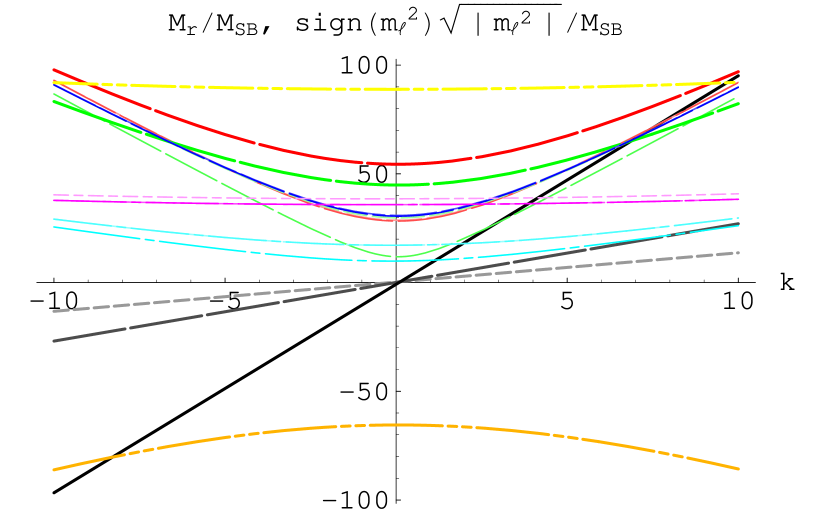
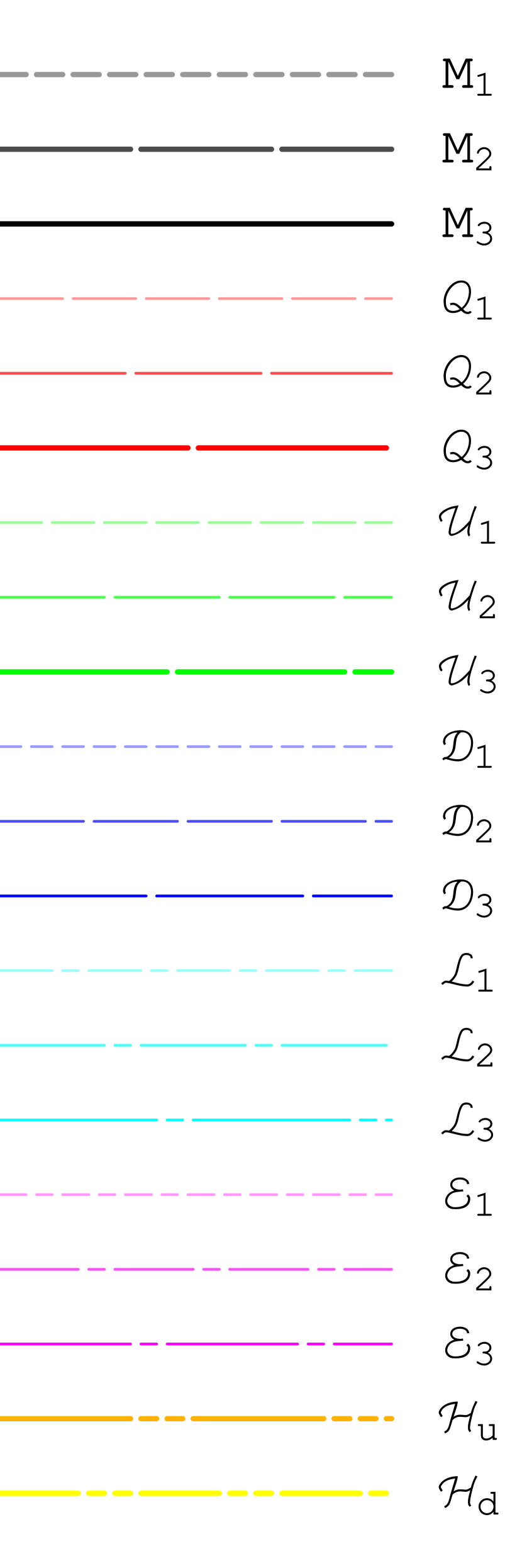
Figure 2: The gaugino masses $M_{r}$ and the scalar masses $m^{2}_{l}$ at $M_{Z}$ as functions of $k\equiv k_{11}=k_{21}=k_{31}$. The parameters are chosen as $c_{X}{\rm Re}\,T^{1}=7.5$.

Rotating scalar masses and A-terms into the super-CKM basis, we can estimate the mass insertion parameters at $M_{Z}$ which are defined by (see, e.g., [30, 22])

$$(\delta^{f}_{LL})_{ij}\!\!\! \equiv\!\!\! \frac{\left((V^{f}_{L})^{\dagger}m_{\tilde{f}_{L}}^{2}V^{f}_{L}\right)_{ij}}{\sqrt{(m_{\tilde{f}_{L}}^{2})_{ii}(m_{\tilde{f}_{L}}^{2})_{jj}}},\qquad(\delta^{f}_{RR})_{ij}\equiv\frac{\left((V^{f}_{R})^{\dagger}m_{\tilde{f}_{R}}^{2}V^{f}_{R}\right)_{ij}}{\sqrt{(m_{\tilde{f}_{R}}^{2})_{ii}(m_{\tilde{f}_{R}}^{2})_{jj}}},$$

$$(\delta^{f}_{LR})_{ij}\!\!\! \equiv\!\!\! \frac{v_{f}\left((V^{f}_{L})^{\dagger}\tilde{A}_{f}V^{f}_{R}\right)_{ij}-\mu_{f}\delta_{ij}(m_{f})_{i}}{\sqrt{(m_{\tilde{f}_{L}}^{2})_{ii}(m_{\tilde{f}_{R}}^{2})_{jj}}},\qquad(\delta^{f}_{RL})_{ij}\equiv(\delta^{f}_{LR})^{\dagger}_{ij},$$ (4.42)

where $m_{\tilde{f}_{L,R}}^{2}$ are the diagonal sfermion mass matrices, and $(\tilde{A}_{f})_{ij}=(y_{f})_{ij}(A_{f})_{ij}$ are the scalar trilinear couplings. The fermion index $f$ and the sfermion indices $\tilde{f}_{L,R}$ represent $f=(u,d,e)$, $\tilde{f}_{R}=(\tilde{u},\tilde{d},\tilde{e})$ and $\tilde{f}_{L}=(\tilde{q},\tilde{q},\tilde{l})$, and then $v_{f}=(\sin\beta,\cos\beta,\cos\beta)v$, $\mu_{f}=(\cot\beta,\tan\beta,\tan\beta)\mu$, respectively, where $v\simeq 174$ GeV and $\mu$ is determined by the minimization condition of the Higgs potential. The unitary matrices $V^{f}_{L,R}$ are defined by $(V^{f}_{L})^{\dagger}y_{f}V^{f}_{R}={\rm diag}\,\left((m_{f})_{i}/v_{f}\right)$.

The mass insertion parameters are severely constrained by the experiments of flavor changing processes. Among these parameters, $(\delta^{e}_{LR})_{21}$ might have the severest constraint from the observations of $\mu\to e\gamma$ processes, and $(\delta^{d}_{LL})_{23}$ from $b\to s\gamma$ processes in our model. Although $b\to s\gamma$ is less restrictive than $\mu\to e\gamma$, the former can be relevant because there are large mass splittings between the third generation squarks and the first two generations with our gauging (4.34) and the charge assignment (4.36). For $M_{SB}=100$ GeV and with ${\cal O}(1)$ values of the holomorphic Yukawa couplings $\lambda^{u,d,e}_{ij}$, we find $|(\delta^{e}_{LR})_{21}|\lesssim{\cal O}(10^{-6})$ and $|(\delta^{d}_{LL})_{23}(\delta^{d}_{LR})_{33}|\lesssim{\cal O}(10^{-3})$ within $|k|\leq 10$. Then, roughly speaking, these parameters are typically within the allowed region [22] for $M_{SB}=100$ GeV. We would study these issues in more detail in a separate work [31].

5 Summary

We have studied 4D effective theory of 5D supergravity with multi moduli, focusing on the contact terms between the hidden and the visible hypermultiplets and a resulting flavor structure of the soft SUSY breaking terms induced at tree-level. The essential difference from the single modulus case appears in the Kähler potential.

In the single modulus case, the induced soft scalar masses by the contact term in the Kähler potential tend to be tachyonic at tree-level. This contribution becomes exponentially small when the visible sector is geometrically sequestered from the SUSY breaking sector. In such a case, quantum effects to the soft scalar masses become dominant, and may save the tachyonic masses at tree-level. However, the hierarchical fermion masses by the localized wave functions along the extra dimension is incompatible with such a sequestering structure [16].

In the multi moduli case, on the other hand, due to the exchange of $Z_{2}$-odd vector multiplets there is an additional contribution to the soft scalar masses that does not suppressed even when the quark, lepton multiplets and the SUSY breaking multiplet are localized around the opposite boundaries. This additional contribution can save the tachyonic scalar mass problem in the single modulus case, and can be even flavor universal. The tree-level contribution to the soft scalar masses always dominate over the quantum effects in the multi moduli case.

Based on these generic features, we constructed a concrete model that stabilizes the moduli at a SUSY breaking Minkowski minimum where hierarchical Yukawa couplings are generated. We have shown the low energy sparticle spectrum of this model and analyzed the mass insertion parameters which are relevant to some observables of flavor changing neutral currents. We should stress that, in our model, all the nontrivial structures at low energies are generated dynamically from the parameters of ${\cal O}(1)$ (in the Planck unit), such as the coefficients of the norm function for the vector multiplets, the charges associated with the hypermultiplet gauging and the boundary induced holomorphic Yukawa couplings.

There are a lot of directions to proceed based on our work. It would be interesting to study models with different parameter choices from those we have chosen in this paper [31]. We may also extend the following models to the case with multi moduli, e.g., the models with two compensator hypermultiplets [14], a twisted $SU(2)_{U}$ gauge fixing [32], an anomalous $U(1)$ symmetry [33], moduli mixing nonperturbative effects [34] and the one in which both the moduli $T^{1}$ and $T^{2}$ remain dynamical at low energies [35], and so on. Another direction is to consider higher dimensional supergravity than 5 dimensional, e.g., magnetised extra dimensions [36], magnetised orbifold models [37] which can realize certain localized wavefunctions for the matter fields with a more fundamental origin of the model, i.e., the string theory.

Although our 5D model has no correspondence with a certain string compactification known until now, the study of our simple model would be helpful to understand some basic nature of all the models where the physics beyond (M)SSM is governed by the dynamics in extra dimensions. Of course, our model itself provides a concrete and dynamical example of the physics beyond the standard model.

Acknowledgements

The authors would like to thank Tatsuo Kobayashi for useful comments. This work was supported in part by the Japan Society for the Promotion of Science for Young Scientists No.182496 (H. A.), and by the Special Postdoctoral Researchers Program at RIKEN (Y. S.).

Appendix A $Z_{2}$-odd part of 5D Weyl multiplet

In supergravity, coordinate derivatives are covariantized for the local SUSY transformation by the gravitino. The 4D derivatives $\partial_{\mu}$ appearing in (2.2) are covariantized by the $Z_{2}$-even gravitino $\psi_{\mu{\rm R}}^{i=1}$ in the $N=1$ Weyl multiplet $E_{W}$ when we promote the $d^{4}\theta$ and $d^{2}\theta$ integrals to the $D$- and $F$-term action formulae of the $N=1$ conformal SUGRA formulation [18]. Here the index $i$ denotes the doublet index for $SU(2)_{\mbox{\scriptsize${\mbox{\boldmath$U$}}$}}$. On the other hand, the derivative $\partial_{y}$ explicitly appearing in the superspace action should be covariantized by an $N=1$ multiplet which contains $\psi_{y{\rm R}}^{i=1}$.

Let us first consider $\partial_{y}$ appearing in the third line in (2.2). As mentioned below Eq.(52) in Ref. [8], it should be promoted to the “covariant derivative” $\hat{\partial}_{y}$ written as

$$\hat{\partial}_{y}\equiv\partial_{y}+\Psi^{\alpha}D_{\alpha}+\Xi^{\mu}\partial_{\mu},$$ (A.1)

where $\Psi^{\alpha}$ and $\Xi^{\mu}$ are $N=1$ superfields with 4D spinor and vector indices. In order for $\hat{\partial}_{y}\Phi^{\hat{a}}$ to be a chiral superfield, $\Psi^{\alpha}$ and $\Xi^{\mu}$ should satisfy the conditions:

$$\bar{D}_{\dot{\alpha}}\Psi^{\alpha}=0,\;\;\;\Psi^{\alpha}=\frac{i}{8}\bar{D}_{\dot{\alpha}}\Xi^{\mu}\bar{\sigma}_{\mu}^{\dot{\alpha}\alpha}.$$ (A.2)

The solution to these conditions is

$$\Psi^{\alpha}=\bar{D}^{2}L^{\alpha},\;\;\;\Xi^{\mu}=-4i\sigma_{\alpha\dot{\alpha}}^{\mu}\bar{D}^{\dot{\alpha}}L^{\alpha},$$ (A.3)

where $L^{\alpha}$ is a complex general multiplet with a spinor index, which contains the $Z_{2}$-odd components of the 5D Weyl multiplet. Since the above solution has an ambiguity of adding a chiral superfield $\Omega^{\mu}$ to $\Xi^{\mu}$, we can devide $\Xi^{\mu}$ into two part as

$$\Xi^{\mu}=\Psi^{\mu}+\Omega^{\mu},$$ (A.4)

so that $\Psi^{\mu}$ contains the same component fields as $\Psi^{\alpha}$. The lowest component of $\Psi^{\alpha}$ is identified with $\psi_{y{\rm R}}^{i=1\,\alpha}$.

In order for the Lagrangian (2.2) to be invariant under the gauge transformation: $\Phi^{\hat{a}}\to(e^{2ig\Lambda^{I}t_{I}})^{\hat{a}}_{\;\;\hat{b}}\Phi^{\hat{b}}$, we have to modify the gauge transformation of $\Sigma^{I}$ as

$$\Sigma^{I}\to\Sigma^{I}+\hat{\partial}_{y}\Lambda^{I},$$ (A.5)

while that of $V^{I}$ remains unchanged as $V^{I}\to V^{I}+\Lambda^{I}+\bar{\Lambda}^{I}$. Thus the gauge invariant quantity ${\cal V}^{I}$ defined below (2.3) should also be modified. The naive modification is

$${\cal V}^{I}\equiv-\hat{\partial}_{y}V^{I}+\Sigma^{I}+\bar{\Sigma}^{I}.$$ (A.6)

However this is not real nor gauge invariant. So we further modify the definition of $\hat{\partial}_{y}$ as

$$\hat{\partial}_{y}\equiv\partial_{y}+\Psi^{\alpha}D_{\alpha}+\bar{\Psi}_{\dot{\alpha}}\bar{D}^{\dot{\alpha}}+\frac{i}{4}\Xi^{\mu}\bar{\sigma}_{\mu}^{\dot{\alpha}\alpha}\bar{D}_{\dot{\alpha}}D_{\alpha}+\frac{i}{4}\bar{\Xi}^{\mu}\sigma_{\mu\alpha\dot{\alpha}}D^{\alpha}\bar{D}^{\dot{\alpha}},$$ (A.7)

which reduces to the previous definition (A.1) when it operates on a chiral superfield. With this definition of $\hat{\partial}_{y}$, the quantity ${\cal V}^{I}$ in (A.6) is now real and gauge invariant.

Now we obtain the couplings of the $Z_{2}$-odd part of the 5D Weyl multiplet to the matter fields by replacing $\partial_{y}$ explicitly appearing in (2.2) with $\hat{\partial}_{y}$ defined in (A.7). In fact, the terms involving $L^{\alpha}$ are necessary for reproducing the correct coefficient functions of the kinetic terms for the gauge fields, $-(1/2)({\cal N}_{IJ}-{\cal N}_{I}{\cal N}_{J}/{\cal N})$, where the arguments of ${\cal N}$’s are the real scalar components of the 5D vector multiplets. If $\partial_{y}$ is not promoted to $\hat{\partial}_{y}$ in the 5D action, the reproduced coefficient functions become incorrect ones, $-(1/2){\cal N}_{IJ}$, as mentioned in Appendix B of Ref. [9]. As a further nontrivial cross-check, we can also see that the couplings of $\Omega_{\mu}$ to the matter multiplets reproduce the correct matter couplings of $V_{\mu}^{(1)}+iV_{\mu}^{(2)}$, which are the $Z_{2}$-odd components of the $SU(2)_{\mbox{\scriptsize${\mbox{\boldmath$U$}}$}}$ (auxiliary) gauge field, if the $F$-term of $\Omega_{\mu}$ is identified as $2i(V_{\mu}^{(1)}+iV_{\mu}^{(2)})$.

As we can see from (A.7) with (A.3), the $Z_{2}$-odd part of the 5D Weyl multiplet couples to the matter multiplets only in the derivative forms. Thus we can neglect their effects on the low-energy effective theory.

Appendix B Derivation of effective Kähler potential

Here we explain the derivation of the Kähler potential in the 4D effective theory shown in (2.14) with (2.15). From (2.10) with (2.12), the effective Kähler potential is written as

$$\Omega\equiv-3e^{-K/3}=-3\int_{0}^{\pi R-\epsilon}\!\!dy\;\hat{{\cal N}}^{1/3}\left(1-\sum_{i}e^{2c_{i}\tilde{V}^{1}}\left|Q_{i}\right|^{2}-\sum_{\alpha}e^{2c_{\alpha}\tilde{V}^{2}}\left|S_{\alpha}\right|^{2}\right)^{2/3},$$ (B.1)

where the arguments of $\hat{{\cal N}}$ is $(-\partial_{y}\tilde{V}^{1},-\partial_{y}\tilde{V}^{2})$. The equation of motion for $\tilde{V}^{1}$ are read off from (2.10) as

$$\hat{{\cal N}}^{1/3}\frac{\sum_{i}4c_{i}e^{2c_{i}\tilde{V}^{1}}\left|Q_{i}\right|^{2}}{\left(1-\sum_{i}e^{2c_{i}\tilde{V}^{1}}\left|Q_{i}\right|^{2}-\sum_{\alpha}e^{2c_{\alpha}\tilde{V}^{2}}\left|S_{\alpha}\right|^{2}\right)^{1/3}}$$

$$-\partial_{y}\left\{\frac{\hat{{\cal N}}_{1}}{\hat{{\cal N}}^{2/3}}\left(1-\sum_{i}e^{2c_{i}\tilde{V}^{1}}\left|Q_{i}\right|^{2}-\sum_{\alpha}e^{2c_{\alpha}\tilde{V}^{2}}\left|S_{\alpha}\right|^{2}\right)^{2/3}\right\}=0.$$ (B.2)

In the absence of the matter multiplets $Q_{i}$ and $S_{\alpha}$, the above equation is reduced to

$$\partial_{y}\left(\frac{\hat{{\cal N}}_{1}}{\hat{{\cal N}}^{2/3}}\right)=0.$$ (B.3)

Note that $\hat{{\cal N}}_{I^{\prime}}/\hat{{\cal N}}^{2/3}$ ($I^{\prime}=1,2$) depends only on the ratio $v\equiv\partial_{y}\tilde{V}^{2}/\partial_{y}\tilde{V}^{1}$, i.e.,

$${\cal F}_{I^{\prime}}(v)\equiv\frac{\hat{{\cal N}}_{I^{\prime}}}{\hat{{\cal N}}^{2/3}}.$$ (B.4)

Thus (B.3) means that $v\equiv\bar{v}$, where $\bar{v}$ is independent of $y$. Then, from the definition of $v$, we obtain a relation:

$$\partial_{y}\tilde{V}^{2}=\bar{v}\partial_{y}\tilde{V}^{1}.$$ (B.5)

By integrating this for $y$ over $[0,\pi R)$, the quantity $\bar{v}$ is determined as

$$\bar{v}=\frac{{\rm Re}\,T^{2}}{{\rm Re}\,T^{1}}.$$ (B.6)

We have used (2.8) and (2.9). In the presence of $Q_{i}$ and $S_{\alpha}$, the ratio $v$ is expanded in terms of them as

$$v\!\!\! =\!\!\! \bar{v}+\sum_{i}A_{i}\left|Q_{i}\right|^{2}+\sum_{\alpha}B_{\alpha}\left|S_{\alpha}\right|^{2}+\sum_{i,j}C_{ij}\left|Q_{i}\right|^{2}\left|Q_{j}\right|^{2}$$ (B.7)

$$+\sum_{i,\alpha}D_{i\alpha}\left|Q_{i}\right|^{2}\left|S_{\alpha}\right|^{2}+\sum_{\alpha,\beta}E_{\alpha\beta}\left|S_{\alpha}\right|^{2}\left|S_{\beta}\right|^{2}+{\cal O}(\hat{\Phi}^{6}),$$

where $\hat{\Phi}=Q_{i},S_{\alpha}$. The coefficients $A_{i}$, $B_{\alpha}$, $C_{ij}$, $D_{i\alpha}$ and $E_{\alpha\beta}$ are independent of $Q_{i}$ and $S_{\alpha}$, which satisfy

$$\int_{0}^{\pi R}\!\!dy\;\left(\sum_{i}A_{i}\left|Q_{i}\right|^{2}+\sum_{\alpha}B_{\alpha}\left|S_{\alpha}\right|^{2}+\sum_{i,j}C_{ij}\left|Q_{i}\right|^{2}\left|Q_{j}\right|^{2}\right.$$

$$\hskip 56.9055pt\left.+\sum_{i,\alpha}D_{i\alpha}\left|Q_{i}\right|^{2}\left|S_{\alpha}\right|^{2}+\sum_{\alpha,\beta}E_{\alpha\beta}\left|S_{\alpha}\right|^{2}\left|S_{\beta}\right|^{2}\right)\partial_{y}\tilde{V}^{1}={\cal O}(\hat{\Phi}^{6}).$$ (B.8)

From (B.1) and (B.7), we obtain

$$\Omega\!\!\! =\!\!\! 3\int_{0}^{\pi R-\epsilon}\!\!dy\;\hat{{\cal N}}^{1/3}(1,v)\partial_{y}\tilde{V}^{1}\left(1-\sum_{i}e^{2c_{i}\tilde{V}^{1}}\left|Q_{i}\right|^{2}-\sum_{\alpha}e^{2c_{\alpha}\tilde{V}^{2}}\left|S_{\alpha}\right|^{2}\right)^{2/3}$$ (B.9)

$$=\!\!\! -3\hat{{\cal N}}^{1/3}(1,\bar{v})\left\{{\rm Re}\,T^{1}-\sum_{i}\frac{1-e^{-2c_{i}{\rm Re}\,T^{1}}}{3c_{i}}\left|Q_{i}\right|^{2}-\sum_{\alpha}\frac{1-e^{-2c_{\alpha}{\rm Re}\,T^{2}}}{3c_{\alpha}\bar{v}}\left|S_{\alpha}\right|^{2}\right.$$

$$\hskip 71.13188pt-\sum_{i,j}\frac{1-e^{-2(c_{i}+c_{j}){\rm Re}\,T^{1}}}{18(c_{i}+c_{j})}\left|Q_{i}\right|^{2}\left|Q_{j}\right|^{2}-\sum_{i,\alpha}\frac{1-e^{-2(c_{i}+c_{\alpha}\bar{v}){\rm Re}\,T^{1}}}{9(c_{i}+c_{\alpha}\bar{v})}\left|Q_{i}\right|^{2}\left|S_{\alpha}\right|^{2}$$

$$\hskip 71.13188pt\left.-\sum_{\alpha,\beta}\frac{1-e^{-2(c_{\alpha}+c_{\beta}){\rm Re}\,T^{2}}}{18(c_{\alpha}+c_{\beta})\bar{v}}\left|S_{\alpha}\right|^{2}\left|S_{\beta}\right|^{2}\right\}$$

$$+\sum_{i,j}\int_{0}^{\pi R}\!\!dy\;\left\{-{\cal F}_{2}(\bar{v})A_{i}\partial_{y}\left(\frac{e^{2c_{j}\tilde{V}^{1}}}{3c_{j}}\right)+\frac{{\cal F}^{\prime}_{2}(\bar{v})}{2}A_{i}A_{j}\partial_{y}\tilde{V}^{1}\right\}\left|Q_{i}\right|^{2}\left|Q_{j}\right|^{2}$$

$$+\sum_{i,\alpha}\int_{0}^{\pi R}\!\!dy\;\left\{{\cal F}_{1}(\bar{v})A_{i}\partial_{y}\left(\frac{e^{2c_{\alpha}\tilde{V}^{2}}}{3c_{\alpha}\bar{v}^{2}}\right)-{\cal F}_{2}(\bar{v})B_{\alpha}\partial_{y}\left(\frac{e^{2c_{i}\tilde{V}^{1}}}{3c_{i}}\right)\right.$$

$$\hskip 71.13188pt\left.+{\cal F}^{\prime}_{2}(\bar{v})A_{i}B_{\alpha}\partial_{y}\tilde{V}^{1}\right\}\left|Q_{i}\right|^{2}\left|S_{\alpha}\right|^{2}$$

$$+\sum_{\alpha,\beta}\int_{0}^{\pi R}\!\!dy\;\left\{{\cal F}_{1}(\bar{v})B_{\alpha}\partial_{y}\left(\frac{e^{2c_{\beta}\tilde{V}^{2}}}{3c_{\beta}\bar{v}^{2}}\right)+\frac{{\cal F}^{\prime}_{2}(\bar{v})}{2}B_{\alpha}B_{\beta}\partial_{y}\tilde{V}^{1}\right\}\left|S_{\alpha}\right|^{2}\left|S_{\beta}\right|^{2}+{\cal O}(\hat{\Phi}^{6}).$$

Here we have used the identity,

$${\cal F}_{1}(v)+v{\cal F}_{2}(v)=3\hat{{\cal N}}^{1/3}(1,v).$$ (B.10)

In order to calculate the remaining integrals in (B.9), we will express $A_{i}$ and $B_{\alpha}$ in terms of $\tilde{V}^{1}$ and $\tilde{V}^{2}$. First, we divide them as

$$A_{i}=A_{i0}+\Delta A_{i},\;\;\;B_{\alpha}=B_{\alpha 0}+\Delta B_{\alpha},$$ (B.11)

where $A_{i0}\equiv A_{i}(y=0)$ and $B_{\alpha 0}\equiv B_{\alpha}(y=0)$. In the absence of $Q_{i}$, (B.2) is reduced to

$$\partial_{y}\left\{{\cal F}_{1}(v)\left(1-\sum_{\alpha}e^{2c_{\alpha}\tilde{V}^{2}}\left|S_{\alpha}\right|^{2}\right)^{2/3}\right\}=0,$$ (B.12)

which means that

$${\cal F}_{1}(v)\left(1-\sum_{\alpha}e^{2c_{\alpha}\tilde{V}^{2}}\left|S_{\alpha}\right|^{2}\right)^{2/3}={\cal F}_{1}(v_{0})\left(1-\sum_{\alpha}\left|S_{\alpha}\right|^{2}\right)^{2/3},$$ (B.13)

where $v_{0}\equiv v(y=0)$. Comparing the coefficients of $\left|S_{\alpha}\right|^{2}$ in both sides, we obtain

$$e^{2c_{\alpha}\tilde{V}^{2}}=1+\frac{3{\cal F}^{\prime}_{1}(\bar{v})}{2{\cal F}_{1}(\bar{v})}\Delta B_{\alpha}+{\cal O}(\left|S_{\alpha}\right|^{2}).$$ (B.14)

Similar relations are derived for $\tilde{V}^{1}$ and $\Delta A_{i}$. In the presence of both $Q_{i}$ and $S_{\alpha}$, they are modified as

$$\Delta A_{i}\!\!\! =\!\!\! \frac{2{\cal F}_{2}(\bar{v})}{3{\cal F}^{\prime}_{2}(\bar{v})}\left(e^{2c_{i}\tilde{V}^{1}}-1\right)+{\cal O}(\left|Q_{i}\right|^{2},\left|S_{\alpha}\right|^{2}),$$

$$\Delta B_{\alpha}\!\!\! =\!\!\! \frac{2{\cal F}_{1}(\bar{v})}{3{\cal F}^{\prime}_{1}(\bar{v})}\left(e^{2c_{\alpha}\tilde{V}^{2}}-1\right)+{\cal O}(\left|Q_{i}\right|^{2},\left|S_{\alpha}\right|^{2}).$$ (B.15)

From (B.8) with these relations, we can determine $A_{i0}$ and $B_{\alpha 0}$ as

$$A_{i0}\!\!\! =\!\!\! \frac{2{\cal F}_{2}(\bar{v})}{3{\cal F}^{\prime}_{2}(\bar{v})}\left(1-\frac{1-e^{-2c_{i}{\rm Re}\,T^{1}}}{2c_{i}{\rm Re}\,T^{1}}\right)+{\cal O}(\left|Q_{i}\right|^{2},\left|S_{\alpha}\right|^{2}),$$

$$B_{\alpha 0}\!\!\! =\!\!\! \frac{2{\cal F}_{1}(\bar{v})}{3{\cal F}^{\prime}_{1}(\bar{v})}\left(1-\frac{1-e^{-2c_{\alpha}{\rm Re}\,T^{2}}}{2c_{\alpha}{\rm Re}\,T^{2}}\right)+{\cal O}(\left|Q_{i}\right|^{2},\left|S_{\alpha}\right|^{2}).$$ (B.16)

Now we can calculate the remaining integrals in (B.9) at the leading order of the $|\hat{\Phi}|^{2}$-expansion by using (B.15) and (B.16). Since we can use a relation $\partial_{y}\tilde{V}^{2}=\bar{v}\partial\tilde{V}^{1}$ in front of the quartic terms in (B.9), the integrands can be rewritten as total derivatives for $y$. After somewhat lengthy calculations, we obtain the expression of $\Omega$ in (2.14) with (2.15). Here we have used the following identities.

$${\cal F}^{\prime}_{1}(v)+v{\cal F}^{\prime}_{2}(v)=0,$$ (B.17)

$${\cal F}^{\prime}_{1}(\bar{v})\!\!\! =\!\!\! {\rm Re}\,T^{1}\partial_{{\rm Re}\,T^{2}}\left(\frac{\hat{{\cal N}}_{1}}{\hat{{\cal N}}^{2/3}}\right)={\rm Re}\,T^{1}\cdot\frac{3\hat{{\cal N}}\hat{{\cal N}}_{12}-2\hat{{\cal N}}_{1}\hat{{\cal N}}_{2}}{3\hat{{\cal N}}^{5/3}},$$ (B.18)

$$3\hat{{\cal N}}\hat{{\cal N}}_{12}-2\hat{{\cal N}}_{1}\hat{{\cal N}}_{2}\!\!\! =\!\!\! -\frac{1}{\bar{v}}\left(3\hat{{\cal N}}\hat{{\cal N}}_{11}-2\hat{{\cal N}}_{1}^{2}\right)$$ (B.19)

$$=\!\!\! -\bar{v}\left(3\hat{{\cal N}}\hat{{\cal N}}_{22}-2\hat{{\cal N}}_{2}^{2}\right).$$

The arguments of $\hat{{\cal N}}$, $\hat{{\cal N}_{I^{\prime}}}$ and $\hat{{\cal N}}_{I^{\prime}J^{\prime}}$ are $({\rm Re}\,T^{1},{\rm Re}\,T^{2})$.

Finally we comment on a special case in which all the gauge couplings $c_{i},c_{\alpha}$ vanish. In this case, $\tilde{V}^{I^{\prime}}$ appear in the action (2.10) only through $\partial_{y}\tilde{V}^{I^{\prime}}$. Then the equation of motion (B.2) is reduced to (B.3), which means that $v=\bar{v}$. Thus the $y$-integral in (B.1) can be easily performed as

$$\Omega\!\!\! =\!\!\! 3\int_{0}^{\pi R}\!\!dy\;\partial_{y}\tilde{V}^{1}\hat{{\cal N}}^{1/3}(1,\bar{v})\left(1-\sum_{i}\left|Q_{i}\right|^{2}-\sum_{\alpha}\left|S_{\alpha}\right|^{2}\right)^{2/3}$$ (B.20)

$$=\!\!\! -3{\rm Re}\,T^{1}\hat{{\cal N}}^{1/3}(1,\bar{v})\left(1-\sum_{i}\left|Q_{i}\right|^{2}-\sum_{\alpha}\left|S_{\alpha}\right|^{2}\right)^{2/3}$$

$$=\!\!\! -3\hat{{\cal N}}^{1/3}({\rm Re}\,T)\left(1-\sum_{i}\left|Q_{i}\right|^{2}-\sum_{\alpha}\left|S_{\alpha}\right|^{2}\right)^{2/3}.$$

Therefore we can obtain the full form of $\Omega$ without expanding by $|\hat{\Phi}|^{2}$ in this case.

References

- [1] I. Antoniadis, N. Arkani-Hamed, S. Dimopoulos and G.R. Divali, Phys. Lett. B436 (1998) 257 [hep-ph/9804398]; N. Arkani-hamed, S. Dimopoulos and G.R Dvali, Phys. Rev. D59 (1999) 086004 [hep-ph/9807344].
- [2] L. Randall and R. Sundrum, Phys. Rev. Lett. 83 (1999) 3370 [hep-ph/9905221].
- [3] N. Arkani-hamed and M. Schmaltz, Phys. Rev. D61 (2000) 033005 [hep-ph/9903417]; D.E. Kaplan and T.M.P. Tait, JHEP 0006 (2000) 020 [hep-ph/0004200].
- [4] M. Zucker, Nucl. Phys. B570 (2000) 267 [hep-th/9907082]; JHEP 0008 (2000) 016 [hep-th/9909144].
- [5] T. Kugo and K. Ohashi, Prog. Theor. Phys. 105 (2001) 323 [hep-ph/0010288]; T. Fujita and K. Ohashi, Prog. Theor. Phys. 106 (2001) 221 [hep-th/0104130]; T. Fujita, T. Kugo and K. Ohashi, Prog. Theor. Phys. 106 (2001) 671 [hep-th/0106051].
- [6] T. Kugo and K. Ohashi, Prog. Theor. Phys. 108 (2002) 203 [hep-th/0203276].
- [7] H. Abe and Y. Sakamura, Phys. Rev. D75 (2007) 025018 [hep-th/0610234].
- [8] F. Paccetti Correia, M. G. Schmidt and Z. Tavartkiladze, Nucl. Phys. B709 (2005) 141 [hep-th/0408138].
- [9] H. Abe and Y. Sakamura, JHEP 0410 (2004) 013 [hep-th/0408224].
- [10] H. Abe and Y. Sakamura, Phys. Rev. D71 (2005) 105010 [hep-th/0501183]; Phys. Rev. D73 (2006) 125013 [hep-th/0511208].
- [11] F. P. Correia, M. G. Schmidt and Z. Tavartkiladze, Nucl. Phys. B751 (2006) 222 [hep-th/0602173].
-
[12]
R. Altendorfer, J. Bagger and D. Nemeschansky,
Phys. Rev. D63 (2001) 125025 [
hep-th/0003117]; A. Falkowski, Z. Lalak and S. Pokorski, Phys. Lett. B491 (2000) 172 [hep-th/0004093]; T. Gherghetta and A. Pomarol, Nucl. Phys. B586 (2000) 141 [hep-ph/0003129]. - [13] A. Lukas, B.A. Ovrut, K.S. Stelle and D. Waldram, Phys. Rev. D59 (1999) 086001 [hep-th/9803235]; Nucl. Phys. B552 (1999) 246 [hep-th/9806051].
- [14] H. Abe and Y. Sakamura, Nucl. Phys. B796 (2008) 224 [arXiv:0709.3791].
- [15] M. Luty and R. Sundrum, Phys. Rev. D62 (2000) 035008 [hep-th/9910202]; Phys. Rev. D64 (2001) 065012 [hep-th/0012158].
- [16] H. Abe, T. Higaki, T. Kobayashi and Y. Omura, JHEP 0804 (2008) 072 [arXiv:0801.0998].
- [17] H. Abe, T. Higaki, T. Kobayashi and Y. Omura, Phys. Rev. D75 (2007) 025019 [hep-th/0611024]; H. Abe, T. Higaki and T. Kobayashi, Phys. Rev. D76 (2007) 105003 [arXiv:0707.2671].
- [18] M. Kaku, P.K. Townsend and P. Van Nieuwenhuizen, Phys. Rev. Lett. 39 (1977) 1109; Phys. Lett. B69 (1977) 304; Phys. Rev. D17 (1978) 3179; T. Kugo and S. Uehara, Nucl. Phys. B226 (1983) 49; Prog. Theor. Phys. 73 (1985) 235.
- [19] K. Choi, A. Falkowski, H.P. Nilles and M. Olechowski, Nucl. Phys. B718 (2005) 113 [hep-th/0503216].
- [20] V.S. Kaplunovsky and J. Louis, Phys. Lett. B306 (1993) 269 [hep-th/9303040].
- [21] K. Choi, D.Y. Kim, I.W. Kim and T. Kobayashi, Eur. Phys. J. C35 (2004) 267 [hep-ph/0305024].
- [22] H. Abe, K. Choi, K.S. Jeong and K. Okumura, JHEP 0409 (2004) 015 [hep-ph/0407005].
- [23] M.A. Luty and R. Sundrum, Phys. Rev. D64 (2001) 065012 [hep-th/0012158].
- [24] N. Maru and N. Okada, Phys. Rev. D70 (2004) 025002 [hep-th/0312148].
- [25] L. O’Raifeartaigh, Nucl. Phys. B96 (1975) 331.
- [26] R. Kallosh and A. Linde, JHEP 0702 (2007) 002 [hep-th/0611183]; R. Kitano, Phys. Lett. B641 (2006) 203 [hep-ph/0607090].
- [27] H. Abe, T. Higaki and T. Kobayashi, Phys. Rev. D74 (2006) 045012 [hep-th/0606095].
- [28] K. Choi, A. Falkowski, H. P. Nilles, M. Olechowski and S. Pokorski, JHEP 0411 (2004) 076 [hep-th/0411066]; K. Choi, A. Falkowski, H. P. Nilles and M. Olechowski, Nucl. Phys. B718 (2005) 113 [hep-th/0503216].
- [29] L. Randall and R. Sundrum, Nucl. Phys. B557 (1999) 79 [hep-th/9810155]; G. F. Giudice, M. A. Luty, H. Murayama and R. Rattazzi, JHEP 9812 (1998) 027 [hep-ph/9810442].
- [30] M. Misiak, S. Pokorski and J. Rosiek, Adv. Ser. Direct. High Energy Phys. 15 (1998) 795 [hep-ph/9703442].
- [31] H. Abe, et al. in progress.
- [32] H. Abe and Y. Sakamura, JHEP 0602 (2006) 014 [hep-th/0512326]; JHEP 0703 (2007) 106 [hep-th/0702097].
- [33] K. Choi and K. S. Jeong, JHEP 0608 (2006) 007 [hep-th/0605108]; E. Dudas, Y. Mambrini, S. Pokorski and A. Romagnoni, JHEP 0804 (2008) 015 [arXiv:0711.4934].
- [34] H. Abe, T. Higaki and T. Kobayashi, Phys. Rev. D 73 (2006) 046005 [hep-th/0511160].
- [35] H. Abe, T. Higaki and T. Kobayashi, Nucl. Phys. B742 (2006) 187 [hep-th/0512232].
- [36] D. Cremades, L. E. Ibanez and F. Marchesano, JHEP 0405 (2004) 079 [hep-th/0404229].
- [37] H. Abe, T. Kobayashi and H. Ohki, arXiv:0806.4748.