Numerical simulation of optimal transport paths

Abstract.

This article provides numerical simulation of an optimal transport path from a single source to an atomic measure of equal total mass. We first construct an initial transport path, and then modify the path as much as possible by using both local and global minimization algorithms.

1. Introduction

This article aims at providing numerical simulations of optimal transport paths studied earlier in [5],[6],[7] [8] etc. The theory of optimal transport paths was motivated by studying a phenomenon in optimal transportation where a transport system with a branching structure may be more cost efficient than the one with a “linear” structure. Trees, railways, lightning, electric power supply, the circulatory system, the river channel networks, and cardiovascular systems are some common examples. We used the concept of optimal transport paths between probability measures to model such transport systems in [5]. Some related works are [1],[2],[3],[4] and others. Also, in [9], we showed that an optimal transport path is exactly a geodesic in the sense of metric geometry on the metric space of probability measures with a suitable metric. As a result, people are interested in knowing what an optimal transport path look like numerically. This is the motivation of this article. Currently, we are using optimal transport paths generated here to model blood vessel structures found in placentas of human babies and also river channel networks. More application of optimal transport paths is expected in modeling systems simulating what we seen in the nature.

This article is organized as follows. After briefly recalling some preliminary definitions about optimal transport paths, we study algorithms for generating optimal transport paths. The idea is as follows. We first consider how to generate an initial transport path, then study how to reduce the cost by modifying the initial transport path as much as possible. We not only use an algorithm of local minimization but also a global one. Topology of transport paths are not preserved during the modification process. These algorithms do not necessarily provide us a perfect optimal transport path, but it approximate an optimal transport path very well. Using eyes of a human being, the author cannot observe a better transport path than the path generated here.

2. Preliminaries

We first recall some concepts about optimal transport paths between measures as studied in [5]. Let $X$ be a convex compact subset in $\mathbb{R}^{d}$. For any $x\in X$, let $\delta_{x}$ be the Dirac measure centered at $x$. An atomic measure in $X$ is in the form of

$$\sum_{i=1}^{k}a_{i}\delta_{x_{i}}$$

with distinct points $x_{i}\in X$, and $a_{i}>0$ for each $i=1,\cdots,k$. Let $\mathbf{a}$ and $\mathbf{b}$ be two fixed atomic measures in the form of

(2.1) $$\mathbf{a}=\sum_{i=1}^{k}a_{i}\delta_{x_{i}}\text{ and }\mathbf{b}=\sum_{j=1}^{l}b_{j}\delta_{y_{j}}$$

of equal total mass

$$\sum_{i=1}^{k}a_{i}=\sum_{j=1}^{l}b_{j}.$$

Definition 2.1.

A transport path from $\mathbf{a}$ to $\mathbf{b}$ is a weighted directed graph $G$ consists of a vertex set $V\left(G\right)$, a directed edge set $E\left(G\right)$ and a weight function

$$w:E\left(G\right)\rightarrow\left(0,+\infty\right)$$

such that $\left\{x_{1,}x_{2,\cdots,}x_{k}\right\}\cup\left\{y_{1},y_{2},\cdots,y_{l}\right\}\subset V\left(G\right)$ and for any vertex $v\in V\left(G\right),$

(2.2) $$\sum_{\begin{subarray}{c}e\in E\left(G\right)\\ e^{-}=v\end{subarray}}w\left(e\right)=\sum_{\begin{subarray}{c}e\in E\left(G\right)\\ e^{+}=v\end{subarray}}w\left(e\right)+\left\{\begin{array}[]{cc}a_{i},&\text{if }v=x_{i}\text{ for some }i=1,\cdots,k\\ -b_{j},&\text{if }v=y_{j}\text{ for some }j=1,\cdots,l\\ 0,&\text{otherwise}\end{array}\right.$$

where $e^{-}$ and $e^{+}$denotes the starting and ending endpoints of each directed edge $e\in E\left(G\right)$.

Remark 2.2.

The balance equation (2.2) simply means that the total mass flows into $v$ equals to the total mass flows out of $v$. When $G$ is viewed as a polyhedral chain or current, (2.2) can be simply expressed as

$$\partial G=\mathbf{b}-\mathbf{a}\text{.}$$

Let $Path(\mathbf{a},\mathbf{b})$ be the space of all transport paths from $\mathbf{a}$ to $\mathbf{b}$.

Definition 2.3.

For any $\alpha\leq 1$, and any $G\in Path(\mathbf{a},\mathbf{b})$, define

$$\mathbf{M}_{\alpha}\left(G\right):=\sum_{e\in E\left(G\right)}\left[w\left(e\right)\right]^{\alpha}length\left(e\right).$$

In [5, Proposition 2.1], we showed that for any transport path $G\in Path\left(\mathbf{a,b}\right)$, there exists another transport path $\tilde{G}\in Path\left(\mathbf{a,b}\right)$ such that

$$\mathbf{M}_{\alpha}\left(\tilde{G}\right)\leq\mathbf{M}_{\alpha}\left(G\right),$$

vertices $V\left(\tilde{G}\right)\subset V\left(G\right)$ and $\tilde{G}$ contains no cycles. Here, a weighted directed graph $G=\left\{V\left(G\right),E\left(G\right),w:E\left(G\right)\rightarrow(0,1]\right\}$ contains a cycle if for some $k\geq 3$, there exists a list of distinct vertices $\left\{v_{1},v_{2},\cdots,v_{k}\right\}$ in $V\left(G\right)$ such that for each $i=1,\cdots,k$, either the segment $\left[v_{i},v_{i+1}\right]$ or $\left[v_{i+1},v_{i}\right]$ is a directed edge in $E(G)$, with the agreement that $v_{k+1}=v_{1}$. When a directed graph $G$ contains no cycles, it becomes a directed tree.

An $\mathbf{M}_{\alpha}$ minimizer in $Path(\mathbf{a},\mathbf{b})$ is called an optimal transport path from $\mathbf{a},\mathbf{b}$.

3. Simulation of optimal transport paths from a single source

Let $X$ be a convex subset in $\mathbb{R}^{d}$. Given two atomic measures in the form of

(3.1) $$\mathbf{a}=m\delta_{O}\text{ and }\mathbf{b}=\sum_{i=1}^{N}m_{i}\delta_{y_{i}}\text{ with }m=\sum_{i=1}^{N}m_{i}$$

in $X$ of equal total mass, we are interested in seeing what an optimal transport path $G$ from the single source $\mathbf{a}$ to $\mathbf{b}$ look like numerically.

If $N=1$, then $G$ is clearly consisting of only one edge $\left[O,y_{1}\right]$ with weight $m$. If $N=2$, then we can calculate the optimal transport path as follows.

3.1. One source to two targets

Suppose there are two atomic measures

(3.2) $$\mu=m_{O}\delta_{O}\text{ and }\nu=m_{P}\delta_{P}+m_{Q}\delta_{Q},$$

with $m_{O}=m_{P}+m_{Q}$ for three points $P,Q,O$ in the space $X$. To find an optimal transport path from $\mu$ to $\nu$, we need to minimize the function

$$f\left(B\right)=\left(m_{O}\right)^{\alpha}\left|\overrightarrow{OB}\right|+\left(m_{P}\right)^{\alpha}\left|\overrightarrow{BP}\right|+\left(m_{Q}\right)^{\alpha}\left|\overrightarrow{BQ}\right|$$

among all points $B$ in the triangle $\triangle POQ$. Here, we use the notation $\overrightarrow{BP}$ etc. to denote the vector $P-B$ in $X$, and let $\left|\overrightarrow{BP}\right|$ be the magnitude of this vector. Since $f\left(B\right)$ is a continuous function on a compact set, $\ f$ must achieve its minimum at some point $B^{\ast}$. Indeed, we can find $B^{\ast}$ as follows. Suppose $B^{\ast}$ is located in the interior of the triangle $\triangle POQ$, then it must satisfy the balance equation

$$\left(m_{O}\right)^{\alpha}\frac{\overrightarrow{OB}}{\left|\overrightarrow{OB}\right|}+\left(m_{P}\right)^{\alpha}\frac{\overrightarrow{BP}}{\left|\overrightarrow{BP}\right|}+\left(m_{Q}\right)^{\alpha}\frac{\overrightarrow{BQ}}{\left|\overrightarrow{BQ}\right|}=\vec{0}$$

at $B=B^{\ast}$. From it, one can easily find the angles

$$\measuredangle OB^{\ast}P=\theta_{1},\measuredangle OB^{\ast}Q=\theta_{2}\text{ and }\measuredangle PB^{\ast}Q=\theta_{3}$$

where

(3.3) $$\theta_{1}=\cos^{-1}\left(\frac{k_{2}-k_{1}-1}{2\sqrt{k_{1}}}\right),\theta_{2}=\cos^{-1}\left(\frac{k_{1}-k_{2}-1}{2\sqrt{k_{2}}}\right),\theta_{3}=\cos^{-1}\left(\frac{1-k_{1}-k_{2}}{2\sqrt{k_{1}k_{2}}}\right)$$

for

$$k_{1}=\left(\frac{m_{P}}{m_{O}}\right)^{2\alpha},k_{2}=\left(\frac{m_{Q}}{m_{O}}\right)^{2\alpha}\text{.}$$

Let $M$ (and $H$) be the projection of the point $Q$ (and $P$, respectively) along the segment $\overrightarrow{OP}$ (and $\overrightarrow{OQ}$ respectively). Then, the centers $R$ (, and $S$) of the circles passing through the triangles $\triangle OB^{\ast}P$ (and $\triangle OB^{\ast}Q$ respectively) is given by

$$R = \frac{O+P}{2}-\frac{\cot\theta_{1}}{2}\frac{\overrightarrow{QM}}{\left|\overrightarrow{QM}\right|}\left|\overrightarrow{OP}\right|$$

$$S = \frac{O+Q}{2}-\frac{\cot\theta_{2}}{2}\frac{\overrightarrow{PH}}{\left|\overrightarrow{PH}\right|}\left|\overrightarrow{OQ}\right|$$

where

$$\overrightarrow{QM}=\frac{\overrightarrow{OP}\cdot\overrightarrow{OQ}}{\left|\overrightarrow{OP}\right|^{2}}\overrightarrow{OP}-\overrightarrow{OQ}\text{ and }\overrightarrow{PH}=\frac{\overrightarrow{OP}\cdot\overrightarrow{OQ}}{\left|\overrightarrow{OQ}\right|^{2}}\overrightarrow{OQ}-\overrightarrow{OP}.$$

By (3.3),

$$\cot\theta_{1}=\frac{k_{2}-k_{1}-1}{\sqrt{4k_{1}-\left(k_{2}-k_{1}-1\right)^{2}}}\text{ and }\cot\theta_{2}=\frac{k_{1}-k_{2}-1}{\sqrt{4k_{2}-\left(k_{1}-k_{2}-1\right)^{2}}}.$$

Now, $B^{\ast}$ is just the reflection of the point $O$ along the segment $RS$. That is,

$$B^{\ast}=2\left[(1-\lambda)R+\lambda S\right]-O\text{ \ with }\lambda=\frac{\overrightarrow{RO}\cdot\overrightarrow{RS}}{\left|\overrightarrow{RS}\right|^{2}}$$

whenever $B^{\ast}$ is located in the interior of the triangle $\triangle POQ$. Note that a necessary condition for $B^{\ast}$ being located in the interior of the triangle $\triangle POQ$ is the angles must satisfy

$$\measuredangle OQP<\theta_{1}\text{,}\measuredangle OPQ<\theta_{2}\text{ and }\measuredangle POQ<\theta_{3}\text{. }$$

In case the condition fails, we have three degenerate cases. If the angle $\measuredangle POQ\geq\theta_{3}$, then take $B^{\ast}$ to be $O$ and we get a “V-shaped” path. If the angle $\measuredangle OQP\geq\theta_{1}$ and $\measuredangle POQ<\theta_{3}$, then take $B^{\ast}$ to be $Q$. If the angle $\measuredangle OPQ\geq\theta_{2}$ and $\measuredangle POQ<\theta_{3}$, then take $B^{\ast}$ to be $P$.

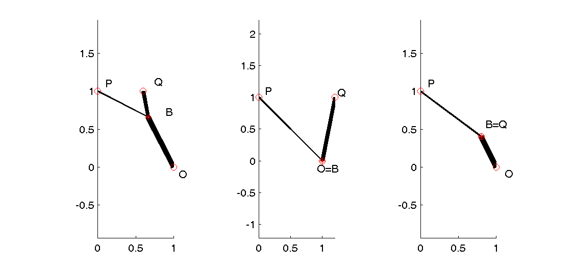
Figure 1. Cases for transporting $\mu$ to $\nu$

As a result, given $\mu$ and $\nu$ in (3.2), we achieved a formula for finding $B^{\ast}$. The optimal transport path $G$ from $\mu$ to $\nu$ has at most three edges: $\left[B^{\ast},P\right]$ with weight $m_{P}$, $\left[B^{\ast},Q\right]$ with weight $m_{Q}$ and $\left[O,B^{\ast}\right]$ with weight $m_{O}$.

We denote the point $B^{\ast}$ by $V\left(\mu,\nu\right)$ and let

(3.4) $$g\left(\mu,\nu\right)=f\left(O\right)-f\left(B^{\ast}\right)$$

which gives the advantage of taking a “Y-shaped” path over taking a “V-shaped” path.

3.2. The construction of an initial transport path

When $N\geq 3$, it is not that easy (or may be impossible) to find an exact solution of an optimal transport path. Instead, we would like to find an approximately optimal transport path. The idea is to construct an initial transport path $G\in Path\left(\mathbf{a,b}\right)$ and then modify $G$ as much as possible until we can not reduce the cost of $G$ any further.

3.2.1. The method of transporting small number of points

If $N\leq 2$, then we have found the optimal transport path $G$ as above. If $2<N\leq K$ for a small given number $K$, then for any pair $1\leq i<j\leq N$, let

$$g_{ij}=g\left(\left(m_{i}+m_{j}\right)\delta_{O},m_{i}\delta_{y_{i}}+m_{j}\delta_{y_{j}}\right)$$

where the function $g$ is defined as in (3.4). Suppose the maximum of $\left\{g_{ij}\right\}$ is achieved at $1\leq i^{\ast}<j^{\ast}\leq N$. Then, the desired path $G$ is given recursively by

$$G=\tilde{G}+m_{i^{\ast}}\left[B^{\ast},y_{i^{\ast}}\right]+m_{j^{\ast}}[B^{\ast},y_{j^{\ast}}],$$

where $B^{\ast}=V\left(\left(m_{i^{\ast}}+m_{j^{\ast}}\right)\delta_{O},m_{i^{\ast}}\delta_{y_{i^{\ast}}}+m_{j^{\ast}}\delta_{y_{j^{\ast}}}\right)$ is the point in $X$ given by (3.4), and $\tilde{G}$ is the path from $\mathbf{a}$ to $\mathbf{\tilde{b}}=\mathbf{b}-m_{i^{\ast}}\delta_{y_{i^{\ast}}}-m_{j^{\ast}}\delta_{y_{j^{\ast}}}+\left(m_{i^{\ast}}+m_{j^{\ast}}\right)\delta_{B^{\ast}}$ achieved by recursively applying this algorithm.

3.2.2. The subdivision method

To construct an initial transport path in $Path\left(\mathbf{a,b}\right)$, one may simply take a trivial transport path

$$\sum_{i=1}^{N}m_{i}\left[O,y_{i}\right].$$

This is an allowable transport path in $Path\left(\mathbf{a,b}\right)$. Nevertheless, the degree of the vertex $O$ (i.e. the total number of edges in $G$ having $O$ as an endpoint) is $N$. Then, it might become time consuming later for modifying the path at the vertex $O$ when $N$ is very large. Instead, we use the following subdivision method to construct an initial transport path $G_{sd}\left(\mathbf{a},\mathbf{b}\right)$, which contains no cycles and has degree at most $K$ at every vertex for some given $K$ defined below.

Let

$$\lambda=\left\{\begin{array}[]{cc}3,&\text{if }d=2\\ 2,&\text{if }d\geq 3\end{array}\right.$$

and $K=\lambda^{d}$ where $d$ is the dimension of the ambient space $\mathbb{R}^{d}$.

Algorithm (subdivision method):

Input: two atomic measures $\mathbf{a},\mathbf{b}$ in the form of (3.1) and a parameter $\alpha\leq 1$;

Output: a transport path $G\in Path\left(\mathbf{a,b}\right)$ with degree$\left(v\right)\leq K$ for each $v\in V(G)$.

If $N\leq K$, then we use the method of transporting small number of points described above to construct a transport path from $\mathbf{a}$ to $\mathbf{b}$.

If $N>K$, then let $Q$ be a cube in $R^{d}$ that contains the supports of both $a$ and $b\,$. We may split the cube $Q$ into totally $K=\lambda^{d}$ smaller cubes $\left\{Q_{i}\right\}_{i=1}^{K}$ of size equal to $\frac{1}{\lambda}$ of the size of $Q$.  For each $i=1,\cdots,K$, let $G_{i}$ be the path $G_{sd}\left(\mathbf{b}\left(Q_{i}\right)\delta_{c\left(Q_{i}\right)},\mathbf{b}\lfloor_{Q_{i}}\right)$ from the center $c\left(Q_{i}\right)$ of the smaller cube $Q_{i}$ to the restriction of $b$ in $Q_{i}$ achieved by recursively applying this algorithm. Also, let $G_{0}$ be the path from $\mathbf{a}$ to $\sum_{i=1}^{K}\mathbf{b}\left(Q_{i}\right)\delta_{c_{\left(Q_{i}\right)}}$ by using the method of transporting small number of points. Then,

$$G=\sum_{i=0}^{K}G_{i}$$

provides the desired path $G_{sd}\left(\mathbf{a},\mathbf{b}\right)$ from $\mathbf{a}$ to $\mathbf{b}$.

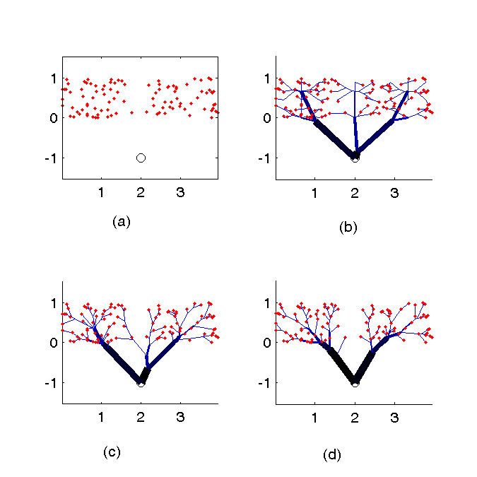
Figure 2. (a) A single source $(2,-1)$ and the targeting measure represented by 100 random points. (b) An initial transport path constructed by the subdivision method. (c)A modified transport path achieved by repeated modifying the initial path in (b) using the local minimization. (d)An optimal transport path achieved by modifying the path in (c) using the global minimization method.

3.3. Modification of an existing transport path

Now, suppose $G$ is an existing transport path from $\mathbf{a}$ to $\mathbf{b}$ that contains no cycles. We want to modify $G$ to reduce the transport cost as much as possible. Before describing algorithms, we first introduce some concepts about vertices of an transport path $G$.

For any two vertices $v,u\in V\left(G\right)$, we say that $v$ is an ancestor of $u$ and $u$ is a descendant of $v$, if there exists a list of vertices $v_{1}=v,v_{2},\cdots,v_{h-1},v_{h}=u$ such that each $\left[v_{i},v_{i+1}\right]$ is a directed edge in $E\left(G\right)$ for $i=1,\cdots,h-1$. Also, if $\left[v,u\right]$ is a directed edge in $E\left(G\right)$, then we say that $v$ is a parent of $u$ and $u$ is a child of $v$.

For each vertex $u\in V\left(G\right)\backslash\left\{O\right\}$, $u$ has exactly one parent $p\left(u\right)\in V\left(G\right)$ because $G$ contains no cycles and has a single source $\mathbf{a}=m\delta_{O}$. Let $m\left(u\right)$ be the associated weight on the directed edge $\left[p\left(u\right),u\right]$ in $E\left(G\right)$ for each $u\in V(G)\setminus\left\{O\right\}$, and also set $m\left(O\right)=m$. Note that $m\left(v\right)\geq m\left(u\right)$ whenever $v$ is an ancestor of $u$. Moreover, the vertex $O$ is always an ancestor of each $u$. That is, there exists a list of vertices $v_{1}$,$v_{2}$,$\cdots,v_{k}$ in $V\left(G\right)$ such that $\left[v_{i},v_{i+1}\right]\in E\left(G\right)$ with $v_{1}=O$ and $v_{k}=u$. Then, for each $t\in\left[-m\left(u\right),m\left(u\right)\right]$, we consider the path

$$R\left(G;t,u\right):=G-\sum_{i=1}^{k-1}t\left[v_{i},v_{i+1}\right]\in Path\left(\mathbf{a}-t\delta_{O}+t\delta_{u},\mathbf{b}\right).$$

When $t>0$, we say that a mass of $t$ is removed from the path $G$ at vertex $u$, When $t<0$, we say that a mass of $t$ is added to the path $G$ at vertex $u$. Moreover, the potential function of $G$ at a vertex $u\in V\left(G\right)$ is defined by

(3.5) $$P_{G}\left(u,t\right)=\left\{\begin{array}[]{cc}P_{G}\left(p\left(u\right),t\right)+\left|p\left(u\right)-u\right|\left[m\left(u\right)^{\alpha}-\left(m\left(u\right)-t\right)^{\alpha}\right],&u\neq O\\ 0,&u=O\end{array}\right.$$

for $t\in\left[-m\left(u\right),m\left(u\right)\right]$. Note that $P_{G}\left(u,t\right)$ has the same sign as $t$.

3.3.1. local minimization

We first use a local minimization method to modify any existing transport path $G$ containing no cycles.

Input: a transport path $G\in Path\left(\mathbf{a,b}\right)$ containing no cycles and $\alpha<1$;

Output: a locally optimized path $\tilde{G}\in Path\left(\mathbf{a,b}\right)$ with $M_{\alpha}\left(\tilde{G}\right)\leq M_{\alpha}\left(G\right)$.

Idea: For each vertex $u$ in $G$, replace $G_{old}\left(u\right)$ by $G_{new}\left(u\right)$ whenever $M_{\alpha}\left(G_{old}\left(u\right)\right)>M_{\alpha}\left(G_{new}\left(u\right)\right)$.

Here, for each vertex $u$ of $G$, two transport paths $G_{old}\left(u\right)$ and $G_{new}\left(u\right)$ are defined as follows. Let

$$\mu_{C}=\sum_{h\in V\left(G\right),p\left(h\right)=u}m\left(h\right)\delta_{h}\text{ and }\mu_{P}=m\left(u\right)\delta_{p\left(u\right)}$$

be two atomic measures corresponding to the children and the parent of $u$. Then,

$$G_{old}\left(u\right)=\sum_{h\in V\left(G\right),p\left(h\right)=u}m\left(h\right)\left[u,h\right]+m\left(u\right)\left[p\left(u\right),u\right]\in Path\left(\mu_{P},\mu_{C}\right)$$

is the union of all weighted edges in $G$ sharing $u$ as their common endpoint. On the other hand, one may generate another path $G_{new}\left(u\right)\in Path\left(\mu_{P},\mu_{C}\right)$ by using the method of transporting small number of points stated in 3.2.1.

If

$$M_{\alpha}\left(G_{old}\left(u\right)\right)>M_{\alpha}\left(G_{new}\left(u\right)\right)\text{,}$$

then by replacing $G_{old}\left(u\right)$ by $G_{new}\left(u\right)$ in $G$, we get a new path

$$\tilde{G}=G-G_{old}\left(u\right)+G_{new}\left(u\right)\in Path\left(\mathbf{a,b}\right)$$

and $M_{\alpha}\left(\tilde{G}\right)\leq M_{\alpha}\left(G\right)-M_{\alpha}\left(G_{old}\left(u\right)\right)+M_{\alpha}\left(G_{new}\left(u\right)\right)<M_{\alpha}\left(G\right)$. So, $\tilde{G}$ is a transport path with less cost. Replace $G$ by this modified path $\tilde{G}$, and continue this process for all vertices of $G$ until one can not reduce the cost any further.

The main drawback of this algorithm is that the result is only local minimization rather than global minimization. For instance, edges may intersect with each other. Sometimes, using eyes of a human being, one can easily observe a better transport path. To overcome these drawbacks, we adopt the following algorithm.

3.3.2. global minimization

Now, we introduce the following algorithm of global minimization:

Input: two probability measures $\mathbf{a}$, $\mathbf{b}$ in the form of (3.1) and a parameter $\alpha\leq 1$;

Output: an approximately $M_{\alpha}$ optimal transport path $G\in Path\left(\mathbf{a,b}\right)$.

step 1: construct a transport path $G$ from $\mathbf{a}$ to $\mathbf{b}$ using the subdivision method;

step 2: modify the existing path $G$ using the local minimization method;

step 3: subdivide long edges of $G$ into shorter edges;

step 4: for each vertex $u$ of $G$, remove a mass of $m\left(u\right)$ at vertex $u$ from the path $G$; change the parent $p(u)$ of $u$ to a better one if possible and then add back a mass of $m\left(u\right)$ at vertex $u$. More precisely,

substep 1: A list of potential parents of $u$ is defined as

$$L\left(u\right)=\left\{v\in V\left(G\right):\left|v-u\right|\leq\sigma\text{, and }v\text{ is not a descendant of }u\right\}\text{,}$$

where

$$\sigma=\frac{P_{G}\left(u,m\left(u\right)\right)}{\left[m\left(u\right)\right]^{\alpha}}$$

and $P_{G}$ is defined in (3.5). Note that the parent $p(u)$ is automatically in $L\left(u\right)$ because

$$\sigma=\frac{P_{G}\left(p(u),m\left(u\right)\right)+\left|p(u)-u\right|m\left(u\right)^{\alpha}}{\left[m\left(u\right)\right]^{\alpha}}\geq\left|p(u)-u\right|.$$

substep 2: By removing a mass of $m\left(u\right)$ at vertex $u$ from the path $G$, we get another path

$$\tilde{G}=R\left(G;m\left(u\right),u\right).$$

substep 3: For each $v\in L\left(u\right)\setminus\left\{p(u)\right\}$, let

$$c\left(v\right)=-P_{\tilde{G}}\left(v,-m\left(u\right)\right),$$

where $P_{\tilde{G}}$ is defined as in (3.5) with $G$ replaced by $\tilde{G}$. The number $c\left(v\right)$ measures the extra cost of transporting a mass of $m\left(u\right)$ on the system $\tilde{G}$ from the source $O$ to the vertex $u$ via the vertex $v$.

substep 4: Find the maximum of $c\left(v\right)$ over all $v\in L\left(u\right)\setminus\left\{p(u)\right\}$. If $\max c\left(v\right)>\sigma\left[m\left(u\right)\right]^{\alpha}$, then we find a better parent for the vertex $u$. In this case, suppose the maximum of $c\left(v\right)$ is achieved at $v^{\ast}$. Then, let

$$G^{\ast}=R\left(\tilde{G};-m\left(u\right),v^{\ast}\right)+m\left(u\right)\left[v^{\ast},u\right].$$

That is, we change the parent of $u$ from $p(u)$ to $v^{\ast}$ and then add a mass $m\left(u\right)$ at the vertex $u$ to the modified path. For convenience, we still denote the final modified transport path $G^{\ast}$ by $G$.

step 5: Repeat steps 2-4 until one can not reduce the cost any further.

4. Examples

Example 4.1.

Let $\left\{y_{i}\right\}$

be 50 random points in the square $\left[0,1\right]\times\left[0,1\right]$. Then, $\left\{y_{i}\right\}$ determines an atomic probability measure

$$\mathbf{b}=\sum_{i=1}^{50}\frac{1}{50}\delta_{y_{i}}.$$

Let $a$$=\delta_{O}$ where $O=\left(0,0\right)$ is the origin. Then an optimal transport path from $\mathbf{a}$ to $\mathbf{b}$ looks like the following figures with $\alpha=1,0.75,0.5$ and $0.25$ respectively:

Example 4.2.

Let $\left\{y_{i}\right\}$ be 100 random points in the rectangle $\left[-2.5,2.5\right]\times\left[0,1\right]$. Then, $\left\{y_{i}\right\}$ determines an atomic probability measure $\mathbf{b}=\sum_{i=1}^{100}\frac{1}{100}\delta_{y_{i}}.$ Let $\mathbf{a}=\delta_{O}$ where $O=\left(0,0\right)$ is the origin, and let $\alpha=0.85$. Then an optimal transport path from $\mathbf{a}$ to $\mathbf{b}$ looks like the following figure.

Example 4.3.

Optimal transport paths from the center to the unit circle. Here, the unit circle is represented by 400 points uniformly distributed on the circle. The parameter $\alpha=0.75$ in the first figure and $\alpha=0.95$ in the second one.

Example 4.4.

Optimal transport paths from the center to the unit disk. The first one is using random generated points in the disk with $\alpha=2/3$ while the second one use uniformly generated points in the disk with $\alpha=0.75$.

Example 4.5.

An optimal transport path from a point on the boundary to the unit square, which is represented by 400 randomly generated points, with $\alpha=0.85$.

Example 4.6.

An optimal transport path modeling blood vessels in a placenta of new baby

References

- [1] A. Brancolini, G. Buttazzo, F. Santambrogio, Path functions over Wasserstein spaces. J. Eur. Math. Soc. Vol. 8, No.3 (2006),415–434.
- [2] Thierry De Pauw and Robert Hardt. Size minimization and approximating problems, Calc. Var. Partial Differential Equations 17 (2003), 405-442.
- [3] E.N. Gilbert, Minimum cost communication networks, Bell System Tech. J. 46, (1967), pp. 2209-2227.
- [4] F. Maddalena, S. Solimini and J.M. Morel. A variational model of irrigation patterns, Interfaces and Free Boundaries, Volume 5, Issue 4, (2003), pp. 391-416.
- [5] Qinglan Xia, Optimal paths related to transport problems. Communications in Contemporary Mathematics. Vol. 5, No. 2 (2003) 251-279.
- [6] Qinglan Xia. Interior regularity of optimal transport paths. Calculus of Variations and Partial Differential Equations. 20 (2004), no. 3, 283–299.
- [7] Qinglan Xia. Boundary regularity of optimal transport paths. Preprint.
- [8] Xia, Qinglan. The formation of tree leaf. ESAIM Control Optim. Calc. Var. 13 (2007), no. 2, 359–377.
- [9] Qinglan Xia. The geodesic problem in nearmetric spaces. Submitted.