Entropy of entanglement and multifractal exponents for random states

Abstract

We relate the entropy of entanglement of ensembles of random vectors to their generalized fractal dimensions. Expanding the von Neumann entropy around its maximum we show that the first order only depends on the participation ratio, while higher orders involve other multifractal exponents. These results can be applied to entanglement behavior near the Anderson transition.

Entanglement is an important characteristics of quantum systems, which has been much studied in the past few years due to its relevance to quantum information and computation. It is a feature that is absent from classical information processing, and a crucial ingredient in many quantum protocols. In the field of quantum computing, it has been shown that a process involving pure states with small enough entanglement can always be simulated efficiently classically jozsa . Thus a quantum algorithm exponentially faster than classical ones requires a minimal amount of entanglement (at least for pure states). Conversely, it is possible to take advantage of the weak entanglement in certain quantum many-body systems to devise efficient classical algorithms to simulate them  cirac . All these reasons make it important to estimate the amount of entanglement present in different types of physical systems, and relate it to other properties of the system. However, in many cases the features specific to a system obscure its generic behavior. One way to circumvent this problem and to extract generic properties is to construct ensembles of systems which after averaging over random realizations can give analytic formulas. Such an approach has proven successful, e.g. in the quantum chaos field, where Random Matrix Theory (RMT) can describe many properties of complex quantum systems.

One of the interesting questions which have been addressed in many studies (see e.g. spins and references therein) is the behavior of entanglement near phase transitions. It has been shown that the entanglement of the ground state changes close to phase transitions. For example, in the XXZ and XY spin chain models, the entanglement between a block of spins and the rest of the system diverges logarithmically with the block size at the transition point kitaev , making classical simulations harder. However, such results cannot be applied directly to systems where the transition concerns one-particle states, for which entanglement has to be suitably defined. A famous example is the Anderson transition of electrons in a disordered potential, which separates localized from extended states, with multifractal states at the transition point. Previous works oneparticle have described the lattice on which the particle evolves as a spin chain and studied entanglement in this framework. However, the lattice can alternatively be described in terms of quantum computation with a much smaller number of two-level systems pom .

In this paper, we study entanglement of random vectors which can be localized, extended or multifractal in Hilbert space. We consider entanglement between blocks of qubits. In the case of the Anderson transition, this amounts to directly relate entanglement to the quantum simulation of the system on a $n_{r}$–qubit system, the number of lattice sites being $2^{n_{r}}$ rather than $n_{r}$ as in oneparticle . Entanglement of random pure states was mainly studied in the case of columns of matrices drawn from the Circular Unitary Ensemble (CUE) CUE . However, such vectors are extended and cannot describe systems with various amounts of localization, from genuine localization to multifractality. Recently it was shown in GirMarGeo ; viola that for localized random vectors, the linear entanglement entropy (first order of the von Neumann entropy) of one qubit with all the others can be related to the localization properties. Here we develop this approach to obtain a general description of bipartite entanglement in terms of certain global properties for random vectors both extended and localized. First we show that for any bipartition, the linear entropy can be written in terms of the participation ratio, a measure of localization. We then show that higher-order terms also depend on higher moments of the wavefunction. In particular, for multifractal systems they are controlled by the multifractal exponents.

Bipartite entanglement of a pure state $|\psi\rangle$ belonging to a Hilbert space ${\mathcal{H}}_{A}\otimes{\mathcal{H}}_{B}$ is measured through the entropy of entanglement, which has been shown to be a unique entanglement measure PopRoh . Let $\rho_{A}$ be the density matrix obtained by tracing subsystem $B$ out of $\rho=|\psi\rangle\langle\psi|$. The entropy of entanglement of the state with respect to the bipartition $(A,B)$ is the von Neumann entropy of $\rho_{A}$, that is $S=-\textrm{tr}(\rho_{A}\log_{2}\rho_{A})$. It is convenient to define the linear entropy as $S_{L}=\frac{d}{d-1}(1-\textrm{tr}\rho_{A}^{2})$, where $d=\dim{\mathcal{H}}_{A}\leq\dim{\mathcal{H}}_{B}$. The scaling factor ensures that $S_{L}$ varies in $[0,1]$. We will show that the average value of $S$ over a set of random states can be expressed only in terms of averages of the moments of the wavefunction

$$p_{q}=\sum_{i=1}^{N}|\psi_{i}|^{2q}$$ (1)

provided some natural assumptions are made. Here we consider ensembles of random vectors of size $N\equiv 2^{n_{r}}$ with the following two properties: i) the phases of the vector components are independent, uniformly distributed random variables, and ii) the joint distribution $P(x_{1},\ldots,x_{N})$ of the modulus squared of the vector components is such that all marginal distributions $P(x_{i})$, $P(x_{i},x_{j})$ for $i\neq j$, $P(x_{i},x_{j},x_{k})$ for $i\neq j\neq k$ and so on, do not depend on the indices. As a consequence, all correlators $\langle|\psi_{i_{1}}|^{2s_{1}}|\psi_{i_{2}}|^{2s_{2}}\ldots\rangle$ of the components of $|\psi\rangle$ are independent of the indices $i_{1}\neq i_{2}\neq\ldots$ involved. Random vectors realized as columns of CUE matrices are instances of vectors having such properties.

Let us first consider the simplest case of entanglement of one qubit with respect to the others. Then $d=2$ and the linear entropy $S_{L}$ is simply the tangle $\tau$, or the square of the generalized concurrence RunCav . It is given by $\tau=4\det\rho_{A}$. If we consider a vector $|\psi\rangle$ of size $N$, the bipartition with respect to qubit $i$ splits the components $\psi_{j}$ of $|\psi\rangle$ into two sets, according to the value of the $i$th bit of the binary decomposition of $j$. If $|\psi^{(0)}\rangle$ and $|\psi^{(1)}\rangle$ are the two corresponding vectors, the linear entropy is

$$\tau=4\left(\langle\psi^{(0)}|\psi^{(0)}\rangle\langle\psi^{(1)}|\psi^{(1)}\rangle-|\langle\psi^{(0)}|\psi^{(1)}\rangle|^{2}\right).$$ (2)

After averaging $\tau$ over random phases, only the diagonal terms survive in the scalar product $|\langle\psi^{(0)}|\psi^{(1)}\rangle|^{2}$. Since it is assumed that two-point correlators of the vector $|\psi\rangle$ do not depend on indices, their average can be expressed solely in terms of the mean moments, as $\langle|\psi_{i}|^{2}|\psi_{j}|^{2}\rangle=\frac{\langle p_{1}^{2}\rangle-\langle p_{2}\rangle}{N(N-1)}$ for $i\neq j$. Normalization of $|\psi\rangle$ implies $p_{1}=1$. As vectors $|\psi^{(0)}\rangle$ and $|\psi^{(1)}\rangle$ always contain components of $|\psi\rangle$ with different indices, we get

$$\langle\tau\rangle=\frac{N-2}{N-1}(1-\langle p_{2}\rangle).$$ (3)

Since $p_{2}=1/\xi$ where $\xi$ is the inverse participation ratio (IPR), Eq. (3) is exactly the Eq. (3) of Ref. GirMarGeo . Let us now turn to the general case, and consider the entropy of entanglement of $\nu$ qubits with $n_{r}-\nu$ others ($(\nu,n_{r}-\nu)$ bipartition). The vector $|\psi\rangle$ is now split into vectors $|\psi^{(j)}\rangle$, $0\leq j\leq 2^{\nu}-1$, depending on the values of the $\nu$ qubits. The reduced density matrix $\rho_{A}$ then appears as the Gram matrix of the $|\psi^{(j)}\rangle$, and the linear entropy is

$$S_{L}=\frac{2^{\nu}}{2^{\nu}-1}\left(1-\sum_{i,j=0}^{2^{\nu}-1}|\langle\psi^{(i)}|\psi^{(j)}\rangle|^{2}\right).$$ (4)

When averaging over random vectors, each term in Eq. (4) with $i\neq j$ yields $2^{n_{r}-\nu}$ two-point correlators, while each term with $i=j$ yields $2^{n_{r}-\nu}(2^{n_{r}-\nu}-1)$ two-point correlators and $2^{n_{r}-\nu}$ terms of the form $\langle|\psi_{i}|^{4}\rangle$. Inserting these expressions into (4) gives $\langle S_{L}\rangle=(N-2^{\nu})(1-\langle p_{2}\rangle)/(N-1)$, which generalizes Eq. (3). The first-order series expansion of the mean von Neumann entropy around its maximum can be expressed as

$$\langle S\rangle\simeq\nu-\frac{2^{\nu}-1}{2\ln 2}\left(1-\frac{N-2^{\nu}}{N-1}\left(1-\langle p_{2}\rangle\right)\right),$$ (5)

with $p_{2}=1/\xi$. Equation (5) shows that for any partition of the system into two subsystems, the average bipartite entanglement of random states only depends at first order on the localization properties of the states, through the mean participation ratio. For CUE vectors, formula (5) reduces to the expression for the mean entanglement derived earlier in Sco . More interestingly, this formula also applies to multifractal quantum states. There, the asymptotic behavior of the IPR is governed by the fractal exponent $D_{2}$, where one defines generalized fractal dimensions $D_{q}$ through the scaling of the moments $p_{q}\propto N^{-D_{q}(q-1)}$. Thus the linear entropy is only sensitive to a single fractal dimension. These results imply that entanglement grows more slowly with the system size for multifractal systems.

To test the relevance of Eq. (5) for describing entanglement in realistic settings, we consider eigenvectors of $N\times N$ unitary matrices of the form

$$U_{kl}=\frac{e^{i\phi_{k}}}{N}\frac{1-e^{2i\pi N\gamma}}{1-e^{2i\pi(k-l+N\gamma)/N}},$$ (6)

where $\phi_{k}$ are independent random variables uniformly distributed in $[0,2\pi[$. These random matrices display intermediate statistical properties bogomolny , and possess eigenvectors that are multifractal MarGirGeo , both features being tuned through the value of the real parameter $\gamma$. We also illustrate Eq. (5) with eigenstates of a many-body Hamiltonian with disorder and interaction $H=\sum_{i}\Gamma_{i}\sigma_{i}^{z}+\sum_{i<j}J_{ij}\sigma_{i}^{x}\sigma_{j}^{x}$. This system can describe a quantum computer in presence of static disorder qchaos . Here the $\sigma_{i}$ are the Pauli matrices for qubit $i$, energy spacing between the two states of qubit $i$ is given by $\Gamma_{i}$ randomly and uniformly distributed in the interval $[\Delta_{0}-\delta/2,\Delta_{0}+\delta/2]$, and the $J_{ij}$ uniformly distributed in the interval $[-J,J]$ represent a random static interaction. For large $J$ and $\delta\approx\Delta_{0}$, eigenstates are delocalized in the basis of register states, but without multifractality. They display properties of quantum chaos, with eigenvalues statistics close to the ones of RMT qchaos . For both systems (unitary matrices and many-body Hamiltonian), components of the eigenvectors have been shuffled in order to reduce correlations, but leaving the peculiarities of the distribution itself unaltered. Figure 1 plots the first-order expansion (5) as a function of the mean IPR for three different bipartitions, showing remarkable agreement with the exact $\langle S\rangle$, both for multifractal (Fig. 1, left panel) and non fractal (right) states, and even for moderately entangled states. The agreement is better for the non-fractal system than for the multifractal one. This can be understood from the study of higher order terms in the entropy.

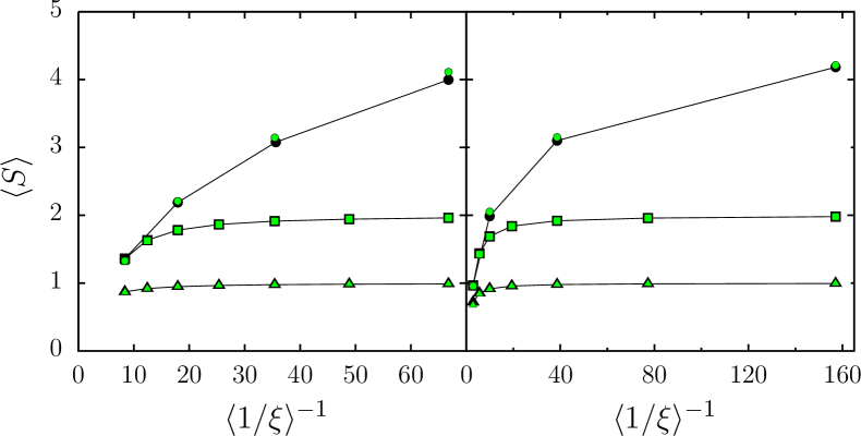
Figure 1: (Color online) Mean entropy of entanglement as a function of the mean IPR. Left: eigenvectors of (6) with $\gamma=1/3$; the average is taken over $10^{6}$ eigenvectors. Right: eigenvectors of the Hamiltonian $H$ (see text) with $\delta=\Delta_{0}$ and $J/\delta=1.5$; average over $N/16$ central eigenstates, with a total number of vectors $\approx 3\times 10^{5}$. Triangles correspond to $\nu=1$, squares to $\nu=2$ and circles to $\nu=n_{r}/2$, with $n_{r}=4-10$ (bipartition of the $\nu$ first qubits with the $n_{r}-\nu$ others). Black symbols are the theoretical predictions for $\langle S\rangle$ at first order (Eq. (5)) and green (grey) symbols are the computed mean values of the exact $\langle S\rangle$.

Indeed, while the linear entropy does not depend on other fractal dimensions than $D_{2}$, the entropy of entanglement does. If we go back to the case of a $(1,n_{r}-1)$ bipartition of the system, the entropy of entanglement can be expressed in a simple way as a function of $\tau$ as

$$S(\tau)=h\left(\frac{1+\sqrt{1-\tau}}{2}\right),$$ (7)

where $h(x)=-x\log_{2}x-(1-x)\log_{2}(1-x)$. The series expansion of $S(\tau)$ up to order $m$ in $(1-\tau)$ reads

$$S_{m}(\tau)=1-\frac{1}{\ln 2}\sum_{n=1}^{m}\frac{(1-\tau)^{n}}{2n(2n-1)}.$$ (8)

The tangle $\tau$ corresponds, up to a linear transformation, to $S_{1}(\tau)$. Let us now calculate the average of higher orders in this expansion. The second-order expansion of $S(\tau)$ involves calculating the mean value of

$$|\langle\psi^{(0)}|\psi^{(1)}\rangle|^{4}=\sum_{i,j,k,l=1}^{N/2}u_{i}^{*}u_{j}u_{k}^{*}u_{l}v_{i}v_{j}^{*}v_{k}v_{l}^{*},$$ (9)

where the star denotes complex conjugation and $u_{i}$, $v_{i}$ are the components of $|\psi^{(0)}\rangle$, $|\psi^{(1)}\rangle$ respectively. Under the assumption of random phases, only terms whose phases cancel survive in (9). Since the phases of all components of $|\psi\rangle$ are independent, cancelation of the phase can only occur if the sets $\{i,k\}$ and $\{j,l\}$ are equal. Thus

$$\langle|\langle\psi^{(0)}|\psi^{(1)}\rangle|^{4}\rangle=2\sum_{\genfrac{}{}{0.0pt}{}{i,k=1}{i\neq k}}^{N/2}\langle|u_{i}u_{k}v_{i}v_{k}|^{2}\rangle+\sum_{i=1}^{N/2}\langle|u_{i}v_{i}|^{4}\rangle.$$ (10)

The correlators in Eq. (10) can be expressed as a function of the moments as follows. Using standard notations MacDo , we will denote by $\lambda\vdash n$ a partition $\lambda=(\lambda_{1},\lambda_{2},\ldots)$ of $n$, with $\lambda_{1}\geq\lambda_{2}\geq\ldots$. For any partition $\lambda\vdash n$, we define $p_{\lambda}=p_{\lambda_{1}}p_{\lambda_{2}}\ldots$, where $p_{\lambda_{i}}$ are given by (1). The monomial symmetric polynomials are defined as $m_{\lambda}=\sum\langle|\psi_{1}|^{2\lambda_{1}}|\psi_{2}|^{2\lambda_{2}}\ldots\rangle$ (the sum runs over all $\mathcal{P}_{\lambda}$ permutations of the $\lambda_{i}$), and we set $c_{\lambda}=m_{\lambda}/\mathcal{P}_{\lambda}$. The $p_{\lambda}$ and $m_{\lambda}$ are related by the simple linear relation $p_{\lambda}=\sum_{\mu}L_{\lambda\mu}m_{\mu}$, where $L_{\lambda\mu}$ is an invertible integer lower-triangular matrix (MacDo , p.103). Upon our assumption ii), any correlator of the form $\langle|\psi_{i_{1}}|^{2s_{1}}|\psi_{i_{2}}|^{2s_{2}}\ldots\rangle$ is equal to a $c_{\lambda}$ for some partition $\lambda$ of $n$, and thus can be expressed as a function of the moments. For instance the two correlators in Eq. (10) are respectively equal to $c_{1111}$ and $c_{22}$. Treating similarly all terms involved in $\tau^{2}$ gives

$$\langle\tau^{2}\rangle = N(N-2)(N^{2}-6N+16)c_{1111}$$

$$+ 4N(N-2)(N-4)c_{211}+4N(N-2)c_{22}.$$

This term involves the calculation of three correlators. Using the relation between the $c_{\lambda}$ and $p_{\lambda}$ and the fact that the vectors are normalized to one we get

$$c_{22} = \frac{\langle p_{2}^{2}\rangle-\langle p_{4}\rangle}{N(N-1)},\ c_{211}=\frac{\langle p_{2}\rangle-\langle p_{2}^{2}\rangle-2\langle p_{3}\rangle+2\langle p_{4}\rangle}{N(N-1)(N-2)},$$

$$c_{1111} = \frac{1-6\langle p_{2}\rangle+8\langle p_{3}\rangle+3\langle p_{2}^{2}\rangle-6\langle p_{4}\rangle}{N(N-1)(N-2)(N-3)}.$$ (12)

The calculation of the general term $\langle\tau^{n}\rangle$ can be performed along the same lines. Expanding (2) we get

$$\tau^{n} = 4^{n}\sum_{k=0}^{n}\binom{n}{k}(-1)^{n-k}$$

$$\times \left(\sum_{i=1}^{N/2}|u_{i}|^{2}\right)^{k}\left(\sum_{i=1}^{N/2}|v_{i}|^{2}\right)^{k}\left(\sum_{i,j}u_{i}^{*}v_{i}u_{j}v_{j}^{*}\right)^{n-k}.$$

The expansion of $\left(\sum_{i,j}u_{i}^{*}v_{i}u_{j}v_{j}^{*}\right)^{t}$ contains products of the form $(u_{i_{1}}\ldots u_{i_{t}})^{*}u_{j_{1}}\ldots u_{j_{t}}$. Only terms where the phases coming from the $u_{i_{k}}^{*}$ compensate those coming from the $u_{j_{k}}$ survive when averaging over random phases. Thus we keep only terms where $\{j_{1},\ldots,j_{t}\}$ is a permutation of $\{i_{1},\ldots,i_{t}\}$. If ${\mathcal{P}}_{K}$ is the number of permutations of a set $K$, the average of (Entropy of entanglement and multifractal exponents for random states) over random vectors reads

$$\langle\tau^{n}\rangle=\Big{\langle}4^{n}\sum_{k=0}^{n}\binom{n}{k}(-1)^{n-k}\sum_{\genfrac{}{}{0.0pt}{}{p_{1},\ldots,p_{k}}{q_{1},\ldots,q_{k}}}\prod_{j=1}^{k}|u_{p_{j}}|^{2}|v_{q_{j}}|^{2}$$

$$\times\sum_{i_{1},\ldots,i_{n-k}}{\mathcal{P}}_{\{i_{1},\ldots,i_{n-k}\}}|u_{i_{1}}v_{i_{1}}|^{2}\ldots|u_{i_{n-k}}v_{i_{n-k}}|^{2}\Big{\rangle}.$$ (14)

Terms with the same correlator can be grouped together. Each correlator in (Entropy of entanglement and multifractal exponents for random states) is some $c_{\lambda\cup\lambda^{\prime}}$, with $\lambda,\lambda^{\prime}$ partitions of $n$. For $\lambda\vdash n$ and $\mu\vdash k$ we define the coefficient $A_{\lambda\mu}=\frac{k!}{\mu!}\sum\frac{(n-k)!}{({\bf s-k})!}$, where the sum runs over all vectors ${\bf s}=(s_{1},\ldots,s_{N/2})$ which are permutations of $\lambda$, and ${\bf k}=(\mu_{1},\ldots,\mu_{N/2})$. We have used the notations $\mathbf{a}=(a_{1},a_{2},\ldots)$ and ${\bf a}!=a_{1}!a_{2}!\ldots$. Finally we get

$$\langle\tau^{n}\rangle=4^{n}\sum_{\lambda,\lambda^{\prime}\vdash n}\bigg{(}\sum_{k=0}^{n}\binom{n}{k}(-1)^{k}\sum_{\mu\vdash k}{\mathcal{P}}_{\mu}A_{\lambda\mu}A_{\lambda^{\prime}\mu}\bigg{)}c_{\lambda\cup\lambda^{\prime}},$$ (15)

which provides an expression for the $n$th order for $\langle S\rangle$ as a function of the $\langle p_{\lambda}\rangle$. In the special case of CUE random vectors, by resumming the whole series we recover after some algebra the well-known result  Pag $\langle S(\tau)\rangle=\frac{1}{\ln 2}\sum_{k=N/2+1}^{N-1}\frac{1}{k}$. Note that similar expressions can be derived for a general $(\nu,n_{r}-\nu)$ bipartition. In this case, the entropy $S=-\textrm{tr}(\rho_{A}\log_{2}\rho_{A})$ can be expanded around the maximally mixed state $\rho_{0}=\mathbf{1}/2^{\nu}$, as

$$S=\nu+\frac{1}{\ln 2}\sum_{n=1}^{\infty}\frac{(-2^{\nu})^{n}}{n(n+1)}\textrm{tr}((\rho_{A}-\rho_{0})^{n+1}).$$ (16)

After averaging over random vectors, one can check that the traces in (16) can be written as $\langle\textrm{tr}\rho_{A}^{k}\rangle=\sum_{\lambda\vdash k}a^{(k)}_{\lambda}c_{\lambda}$, with $a^{(k)}_{\lambda}$ some integer combinatorial coefficient. The entropy can thus be written as a linear combination of $c_{\lambda}$ with rational coefficients that can be expressed in terms of the $a^{(k)}_{\lambda}$.

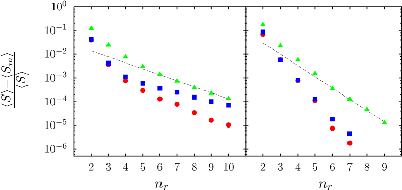
Figure 2: (Color online) Relative difference of the entropy of entanglement (7) and its successive approximations $S_{m}$ ($m=1,2$) with respect to the number of qubits for eigenvectors of (6) for (left) $\gamma=1/3$ and (right) $\gamma=1/7$. The average is taken over $10^{7}$ eigenvectors, yielding an accuracy $\lesssim 10^{-6}$ on the computed mean values. Green triangles correspond to the first-order expansion $S_{1}$, blue squares and red circles to the second-order expansion $S_{2}$. The difference between the latter two is that for blue squares $\langle p_{2}^{2}\rangle$ appearing in Eq. (Entropy of entanglement and multifractal exponents for random states) has been replaced by $\langle p_{2}\rangle^{2}$ yielding a less accurate approximation. Dashed line is a linear fit yielding $1-\langle S_{1}\rangle/\langle S\rangle$ $\sim N^{-0.84}$ for $\gamma=1/3$ and $N^{-1.58}$ for $\gamma=1/7$.

In Fig. 2 we illustrate the accuracy of higher-order terms in the series expansion of $S$ for multifractal random vectors by comparing the first and second-order expansion for eigenvectors of the matrices (6). As expected, the second-order expansion is much more accurate than the first order one and gives a much better estimate of the mean entropy of entanglement already for small system sizes. For large $N$, the dominant term in $S_{2}$ is $\propto\langle p_{2}^{2}\rangle$. Numerically we obtained $\langle p_{2}^{2}\rangle\sim N^{-0.81}$ for $\gamma=1/3$, and $\langle p_{2}^{2}\rangle\sim N^{-1.53}$ for $\gamma=1/7$, which is indeed consistent with the slopes of the linear fit of $\log_{2}(1-\langle S_{1}\rangle/\langle S\rangle)$ (see Fig. 2). If one replaces $\langle p_{2}^{2}\rangle$ appearing in Eq. (Entropy of entanglement and multifractal exponents for random states) by $\langle p_{2}\rangle^{2}$ (squares in Fig. 2), the second-order expansion is now governed only by three multifractal dimensions $D_{2}$, $D_{3}$, $D_{4}$. Although it becomes less and less accurate with the system size because of the increase of the variance of $p_{2}$, it remains a very good improvement over the first order in the case of moderate multifractality (Fig. 2, right).

Our results show that the entanglement of random vectors directly depends on whether they are localized, multifractal or extended. The numerical simulations for different physical examples show that our theory describes well individual systems whose correlations are averaged out. Previous results GirMarGeo have shown that Anderson-localized states have entanglement going to zero for large system size. The present work shows that multifractal states, such as those appearing at the Anderson transition, approach the maximal value of entanglement in a way controlled by the multifractal exponents. Although extended and multifractal states are both close to maximal entanglement, the way multifractal states approach the maximal value for large system size is slower.

The authors thank CalMiP in Toulouse for access to their supercomputers. This work was supported by the Agence Nationale de la Recherche (ANR project INFOSYSQQ, contract number ANR-05-JCJC-0072) and the European program EC IST FP6-015708 EuroSQIP.

References

- (1) R. Jozsa and N. Linden, Proc. R. Soc. London Ser. A 459, 2011 (2003).
- (2) G. Vidal, Phys. Rev. Lett. 91, 147902 (2003); F. Verstraete, D. Porras, and J. I. Cirac, Phys. Rev. Lett. 93, 227205 (2004).
- (3) L. Amico, R. Fazio, A. Osterloh, and V. Vedral, Rev. Mod. Phys. 80, 517 (2008).
- (4) G. Vidal, J. I. Latorre, E. Rico, and A. Kitaev, Phys. Rev. Lett. 90, 227902 (2003).
- (5) L. Gong and P. Tong, Phys. Rev. E 74, 056103 (2006); X. Jia, A. R. Subramaniam, I. A. Gruzberg, and S. Chakravarty, Phys. Rev. B 77, 014208 (2008); I. Varga, J. A. Mendez-Bermudez, Phys. Stat. Sol. (c) 5, 867 (2008).
- (6) A. A. Pomeransky and D. L. Shepelyansky, Phys. Rev. A 69, 014302 (2004).
- (7) H.-J. Sommers and K. Zyczkowski, J. Phys. A 37, 8457 (2004); O. Giraud, ibid. 40, 2793 (2007); M. Znidaric, ibid. 40, F105 (2007).
- (8) L. Viola and W. G. Brown, J. Phys. A 40, 8109 (2007); W. G. Brown, L. F. Santos, D. J. Starling and L. Viola, Phys. Rev. E 77, 021106 (2008).
- (9) O. Giraud, J. Martin, and B. Georgeot, Phys. Rev. A 76, 042333 (2007).
- (10) S. Popescu and D. Rohrlich, Phys. Rev. A 56, R3319 (1997).
- (11) P. Rungta and C. M. Caves, Phys. Rev. A 67, 012307 (2003).
- (12) A. J. Scott, Phys. Rev. A 69, 052330 (2004).
- (13) E. Bogomolny and C. Schmit, Phys. Rev. Lett. 93, 254102 (2004).
- (14) J. Martin, O. Giraud, and B. Georgeot, Phys. Rev. E 77, R035201 (2008).
- (15) B. Georgeot and D. L. Shepelyansky, Phys. Rev. E 62, 3504 (2000); Phys. Rev. E 62, 6366 (2000).
- (16) I. G. Macdonald, Symmetric functions and Hall polynomials, 2nd ed., Oxford University Press (1995).
- (17) D. N. Page, Phys. Rev. Lett. 71, 1291 (1993).