Full-Sky Weak-Lensing Simulation with 70 Billion Particles

We have performed a 70 billion dark-matter particles N–body simulation in a 2 $h^{-1}$ Gpc periodic box, using the concordance, cosmological model as favored by the latest WMAP3 results. We have computed a full-sky convergence map with a resolution of $\Delta\theta\simeq 0.74$ arcmin², spanning 4 orders of magnitude in angular dynamical range. Using various high-order statistics on a realistic cut sky, we have characterized the transition from the linear to the nonlinear regime at $\ell\simeq 1000$ and shown that realistic galactic masking affects high–order moments only below $\ell<200$. Each domain (Gaussian and non–Gaussian) spans 2 decades in angular scale. This map is therefore an ideal tool for testing map–making algorithms on the sphere. As a first step in addressing the full map reconstruction problem, we have benchmarked in this paper two denoising methods: 1) Wiener filtering applied to the Spherical Harmonics decomposition of the map and 2) a new method, called MRLens, based on the modification of the Maximum Entropy Method on a Wavelet decomposition. While the latter is optimal on large spatial scales, where the signal is Gaussian, MRLens outperforms the Wiener method on small spatial scales, where the signal is highly non–Gaussian. The simulated full-sky convergence map is freely available to the community to help the development of new map–making algorithms dedicated to the next generation of weak–lensing surveys.

1 Introduction

Weak gravitational lensing, or “cosmic shear”, provides a unique tool for mapping the matter density distribution in the Universe (for reviews, see Refregier (2003), Hoekstra (2003) and Munshi et al. (2006)). Current weak-lensing surveys cover altogether about 100 square degrees and have been used to measure the amplitude of the matter power spectrum and other cosmological parameters (see Benjamin et al. (2007), Fu et al. (2008) and references therein). A number of new instruments are being planned to carry out these surveys over wider sky areas (PanSTARRS, DES, SNAP and LSST) or even over the full extragalactic sky (DUNE). These wide-field surveys will yield cosmic-shear measurements on both large scales, where gravitational dynamics is in the linear regime, and small scales, where the dynamics is highly nonlinear. The comparison of these measurements with theoretical predictions of the density field evolution will place strong constraints on cosmological parameters, including dark energy parameters (e.g. Hu & Tegmark (1999), Huterer (2002), Amara & Refregier (2006) and Albrecht & Bernstein (2007)). On small scales, the highly nonlinear nature of the density field ensures that predictions based on analytic calculations are prohibitively difficult and requires the use of numerical simulations. N-body simulations have thus been used to simulate weak-lensing maps across small patches of the sky, using the flat sky approximation (e.g. Jain et al. (2000), Hamana et al. (2001) and White & Vale (2004)). The simulation of full-sky maps in preparation for future surveys involve a wide range of both mass and length scales and is challenging for current N-body simulations. The range of scales involved also requires the development of efficient algorithms for deriving a mass map from true noisy data sets. These algorithms need to be well–suited to both the large–scale signal, which is essentially a Gaussian random field, and those on small–scales, where it is highly non–Gaussian and exhibits localized features.

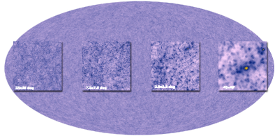
Figure 1: Full-sky simulated convergence map derived from the Horizon Simulation. Its resolution of 200 million pixels has been downgraded to fit the page. The various inserts display a zoom sequence into smaller and smaller areas of the sky. The pixel size is 0.74 arcmin².

In this paper, we used a high resolution N-body simulation to construct a full-sky weak-lensing map and test a new map-reconstruction method based on a multi-resolution technique. For this purpose, we use the Horizon simulation, a 70 billion particle N–body simulation, featuring more than $140$ billion cell in the AMR grid of the RAMSES code (Teyssier 2002). The simulation covers a sufficiently large volume ($L_{box}=2h^{-1}$Gpc) to compute a full-sky convergence map, while resolving Milky-Way size halos with more than 100 particles, and exploring small scales into the nonlinear regime (see Sect. 2). This unprecedented computational effort allows us, for the first time, to close the gap between scales close to the cosmological horizon and scales deep inside virialized dark-matter haloes. A similar effort at lower resolution was presented by Fosalba et al. (2008).

The dark-matter distribution in the simulation was integrated in a light cone to a redshift of 1, around an observer located at the centre of the simulation box (see Sect. 3). This light cone was then used to calculate the corresponding full-sky lensing convergence field, which we mapped using the Healpix pixelisation scheme (Górski et al. 2005) with a pixel resolution of $\Delta\theta\simeq 0.74$ arcmin² ($n_{\rm side}=4096$), and added “instrumental” noise for a typical all–sky survey with 40 galaxies per arcmin², as expected for example for the DUNE mission (Réfrégier et al. 2006). Using an Undecimated Isotropic Wavelet Decomposition of this realistic simulated weak-lensing map on the sphere, we analyzed the statistics of each wavelet plane using second, third and fourth order moments estimator (Sect. 4). We then applied, in Sect. 5, a multi-resolution algorithm to filter a fictitious simulated $\kappa$ data set based on an extension of the wavelet filtering technique of Starck et al. (2006b). We characterised the quality of the reconstruction using the power spectrum of the error map and compare this to the result of standard Wiener filtering on the sphere. Our results, summarised in Sect. 6, illustrate the virtue of high resolution simulations such as the one reported here to prepare for future weak-lensing surveys and to design new map–making techniques.

2 The Horizon N-Body simulation

This large N-body simulation was carried out using the RAMSES code (Teyssier 2002) for two months on the 6144 Itanium2 processors of the CEA supercomputer BULL Novascale 3045 hosted in France by CCRT. RAMSES is a parallel hydro and N-body code based on the Adaptive Mesh Refinement (AMR) techniques. Using a parallel version of the grafic package (Bertschinger 2001), we generated the initial displacement field on a $4096^{3}$ grid for the cosmological parameters from the WMAP 3rd year results (Spergel et al. 2007), namely $\Omega_{m}=0.24$, $\Omega_{\Lambda}=0.76$, $\Omega_{b}=0.042$, $n=0.958$, $H_{0}=73$ km/s/Mpc and $\sigma_{8}=0.77$. We used the Eisenstein & Hu (1999) transfer function, which includes baryon oscillations. The box size was set to 2 Gpc/h, which corresponds roughly to the comoving distance to an object at $z\simeq 0.8$. We used 68.7 billion particles to simuate the dark-matter density field, yielding a particle mass of $7.7\times 10^{9}$ $M_{\odot}$ and 130 particles per Milky Way halo. This large particle distribution was split across 6144 individual files, one for each processor, according to the RAMSES code domain decomposition strategy (Prunet et al. 2008). Starting with a base (or coarse) grid of $4096^{3}$ grid points, AMR cells are recursively refined if the number of particles in the cell exceeds 40. In this way, the number of particles per cell varied between 5 and 40, so that the particle shot noise remained at an acceptable level. At the end of the simulation, we had reached 6 levels of refinement with a total of 140 billion AMR cells. This corresponds to a formal resolution of $262\leavevmode\nobreak\ 144^{3}$ or 7.6 $h^{-1}$ kpc comoving spatial resolution. Parallel computing is perfomed using the MPI message–passing library, with a domain decomposition based on the Peano–Hilbert space–filling curve. The work and memory load was adjusted dynamically by reshuffling particles and grid points from each processor to its neighbors. The simulation required 737 main (or coarse) time steps and more than $10^{4}$ fine time steps for completion.

3 Light cone and convergence map

Born’s unperturbed-trajectory assumption for all neighboring light rays is a good approximation in the linear regime of structure formation, but is inaccurate in the nonlinear regime. Consequently, distortion effects of lensing beyond the first order cannot be simulated reliably. As shown by Van Waerbeke et al. (2001), the Born approximation also introduces a relative error in the skewness of the signal of aproximately 10% on large scales where the convergence is Gaussian, and about 1% on small scales in the nonlinear regime. We therefore implemented a multiple-lens ray-tracing method that can be applied more generally than Born’s approximation.

We constructed a light cone by recording, at each main time step, the positions of particles within the boundaries of a photon plane: this plane moved at the speed of light towards an observer, who was located at the centre of the box. Our method was developed from the one presented by Hamana et al. (2001). This method produced 348 slices in the light cone, spanning the redshift range [0,1]. Due to the large size of the simulated volume, the effect of periodic replications of the computational box are minimized. Each slice was then transformed into a full-sky Healpix map ($nside=4096$) of the average overdensity using a simple “Nearest Grid Point” (NGP) mass projection scheme. The density slices thus represented our physical model of the lens screens used in the ray-tracing procedure. We note that there is no unique procedure for generating a band-limited harmonic representation of each slice of particles. We chooe to use an NGP interpolation because it is a good compromise between filtering and aliasing, and remains localised in configuration space. More sophisticated interpolation schemes have been developed in the context of either 3D particle distributions (Colombi et al. 2008) or 2D continuous fields (Basak et al. 2008), which, however, remain impractical in significantly large simulations.

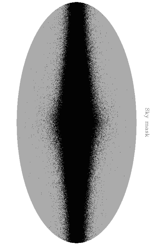
Figure 2: Map of the cut-sky used in Sect. 4 to compute high-order moments.

After an interpolation kernel has been chosen, all fields (lensing potentials and displacement fields) are computed from the NGP interpolation mass slices at each redshift using a spherical harmonic decomposition. The resampling of the displacement fields outside the pixel centres (as required in a multi-lens method) is completed using a local linear-interpolation scheme (using covariant, second derivatives of the potential); this last interpolation has the same spectral behavior (and thus the same aliasing contamination) as the NGP-interpolated mass slices, and we therefore do not need to use a higher-order resampling scheme (since the calculation of the potential requires two sets of integration over the mass distribution, while the interpolation of the displacement field corresponds to a second-order derivative). We provide more details in Appendix A (see Jain et al. (2000), Hamana et al. (2001) and White & Vale (2004) for alternative approaches). We assumed that the background galaxies are within a single source plane located at redshift $z_{s}=1$. The final convergence map was computed using our multiple-lens ray-tracing scheme, for which spherical geometry precludes the use of small angle approximations (as in Das & Bode (2008)) especially in the neighborhood of the poles; full rotation matrices for each light ray must therefore be computed from the displacement fields at each redshift.

The resulting full-sky Healpix map with a pixel size of $\Delta\theta\simeq 0.74$ arcmin is shown in Fig. 1, with small inserts to highlight the large dynamical range achieved. The particle shot noise corresponding to our 70 billion particle run has a small impact on the map. As shown in Fig. 4, the particle shot noise is well below the expected instrumental noise, and even sufficiently low to be ignored in the spectral analysis of the signal.

4 High–order moments and realistic sky cut

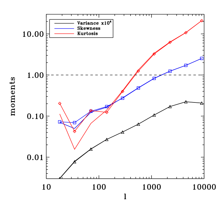
Figure 3: Moments of the convergence as a function of the average multipole moment on each wavelet scale. The variance, skewness, and kurtosis are shown as black, blue, and red lines, respectively. Solid lines with error bars corresponds ro a full-sky analysis, while dotted lines correspond to our cut-sky analysis.

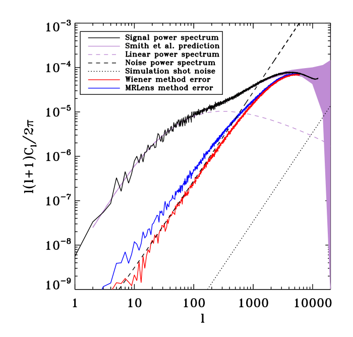
Figure 4: Angular power spectrum of the simulated convergence map (black solid line), compared to a fit based on the Smith et al. (2001) analytical model with error bars corresponding to our noise model (pink area). Also shown is the prediction from linear theory (pink dashed curve). The noise power spectrum is plotted as the dashed black line. The green solid line is the power spectrum of the error map obtained with the Wiener filter method, while the blue solid line are that for the MRLens method.

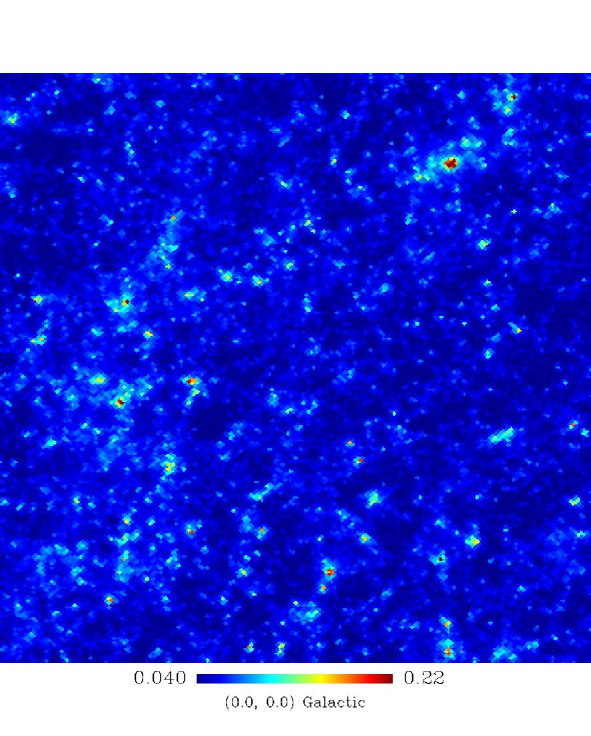
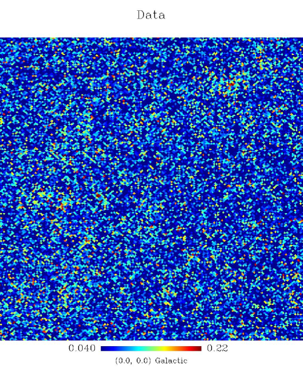
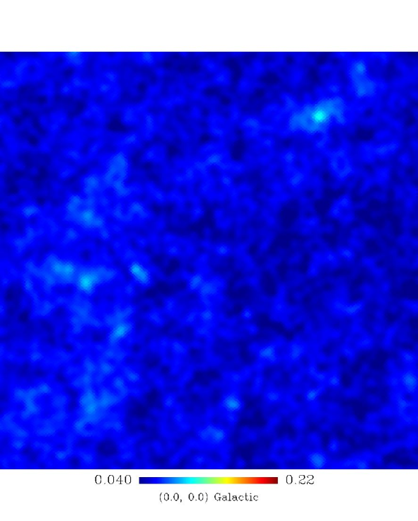
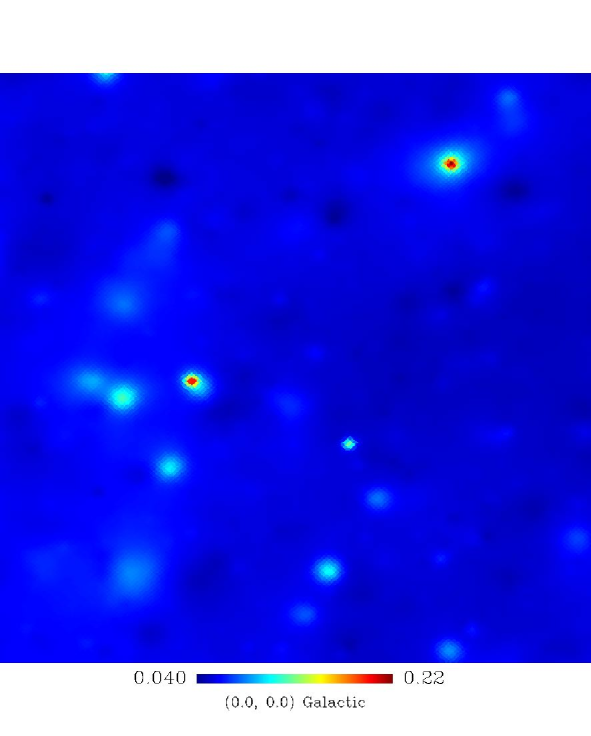
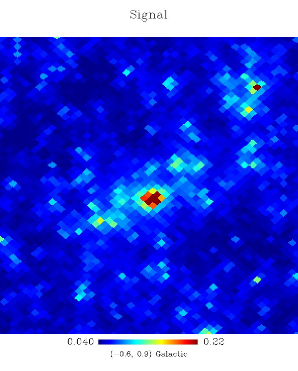
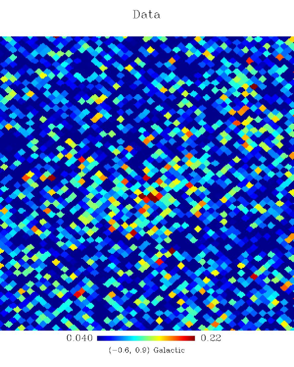
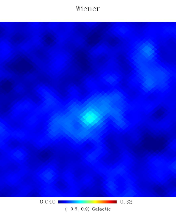
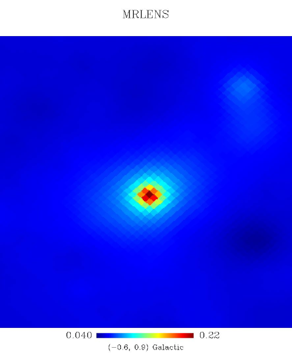
Figure 5: Reconstruction of convergence maps with our 2 filtering techniques. The top panels show the $2.5^{o}\times 2.5^{o}$ square map corresponding to first zoom sequence of Fig. 1. The bottom panels are subset of the corresponding top images with linear size 45${}^{{}^{\prime}}$. From left to right, we show the original signal, the noisy image, the Wiener-filtered image and the the MRLens-filtered image.

In Fig. 1, the signal appears as a typical Gaussian random field on large scales, similar to the Cosmic Microwave Background map seen by the WMAP satellite (Spergel et al. 2007). On small scales, the signal is clearly dominated by clumpy structures (dark matter halos) and is therefore highly non-Gaussian. To characterize this quantitatively, we performed a wavelet decomposition of our map using the Undecimated Isotropic Wavelet Transform on the sphere (Starck et al. 2006a), and, for each wavelet scale, we have computed its second-, third- and fourth-order moment. We used 11 scales with central multipole values of $\ell_{0}=9000$, 4500, 2250, 1125, 562, 282, 141, 71, 35, 18. For each of these maps, we computed the variance $\sigma^{2}=\langle\kappa^{2}\rangle$, the normalized skewness $S=\langle\kappa^{3}\rangle/\sigma^{3}$, and the normalized kurtosis $K=\langle\kappa^{4}\rangle/\sigma^{4}$. Results are plotted in Fig. 3 as solid lines of various colors. Error bars were estimated approximately by computing each moment on the 12 Healpix base pixels independently and evaluating the variance in the 12 results. A more appropriate strategy would have been to perform several, independent, 70 billion particle runs, which is currently impossible for us to do. We can see that the variance in the signal steadily increases for higher and higher multipoles, and saturates at a fraction of $10^{-4}$, corresponding to the value predicted from nonlinear gravitational clustering for $\ell\geq 6000$. The variance for each wavelet plane can be considered to be a band power estimate of the angular power spectrum, as can be verified using Fig. 4. In the same figure, we have also plotted for comparison the linear power spectrum, to highlight the scale below which nonlinear clustering contributes significantly, i.e., for $\ell>750$ or equivalently $\theta<15^{{}^{\prime}}$, as first pointed out by Jain & Seljak (1997). Skewness and kurtosis are more direct estimators of the signal non–Gaussianity. Departures from Gaussianity occur around $\ell\simeq 750-1500$, where both statistics cross unity. Due to the large dynamical range of the Horizon simulation, we computed a map spanning two decades in angular scales in the linear, Gaussian regime and two additional decades in angular scales into the nonlinear, non–Gaussian regime.

It is clear from Fig. 3 that at small $\ell$, the skewness and the kurtosis of the map are strongly affected by cosmic variance. The statistics of the convergence field cannot be measured in practice over the whole sky because of sky cuts imposed by the presence of saturated stars and by absorption in the Galactic plane. We estimated the impact of this sky cut on the accuracy of our multi-resolution statistical analysis. We computed the expected number of bright stars that would saturate CCD cameras typically employed in wide-field survey (B-magnitude$<20$). We then removed from our analysis each pixel contaminated by at least 3 bright stars, based on a random Poissonian realization of bright stars in our Galaxy (according to the model presented in Bahcall & Soneira (1980), Appendix B). We obtain a mask with 40% of the sky removed, corresponding roughly to a $\pm 20^{o}$ cut around the Galactic plane (see Fig. 2). The resulting statistics are overplotted as dotted lines in Fig. 3. The transition scale, for which the departure from Gaussianity is significant, can still be estimated reliabily around $\ell\simeq 750-1500$. We concluded that the cosmic variance of the cut sky affects high–order moments only below $\ell\simeq 200$.

5 Map–making using multi–resolution filtering

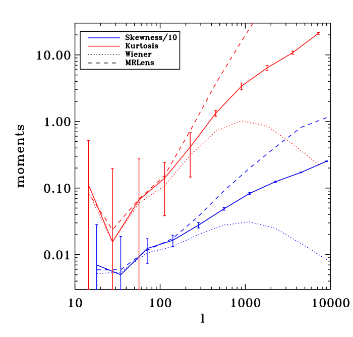
Figure 6: Skewness (blue lines) and kurtosis (red lines) for the original convergence map (solid lines with error bars), compared to the same high-order statistics for the Wiener reconstructed map (dotted lines) and the MRLens reconstructed map (dashed lines).

The full-sky simulated convergence maps described above can be used to analyze and compare de-noising (or map–making) methods on the sphere. For this purpose, we considered a purely white instrumental noise, typical of the next generation all–sky surveys, and a root mean square per pixel of area $A_{p}$ given by $\sigma_{N}=0.3/\sqrt{n_{gal}A_{p}}$ for $n_{gal}=40$ background galaxies per arcmin². Recovering the most accurate convergence map from noisy data will be an important step in future surveys. This reconstructed map can be used to construct a mass selected halo catalog, measure its statistical properties and constrain cosmological parameters, and be compared directly with other cluster catalogues compiled with other techniques (X-ray, galaxy counts or SZ). We restrict ourselves to the full-sky denoising of a convergence map already reconstructed from the shear derived from galaxy ellipticities. In the present work, we do not address filtering in the presence of a cut–sky, such as the one shown in Fig. 2. Promising methods based on “impainting” have been developed in the CMB context (Abrial et al. 2008), and also weak-lensing applications (Pires et al. 2008); these replace missing data with an artificial signal and allow us to optimize the results we obtained with filtering methods for a full-sky analysis.

A straightforward filtering method is the Wiener filtering scheme, which is optimal for Gaussian random fields, and is expected to operate here effectively on large scales. Defining $S_{\ell}$ as the power spectrum of the input signal (see Fig. 4) and $N_{\ell}$ the power spectrum of the noise, this method involves convolving the noisy map by the Wiener filter defined as $W_{\ell}=S_{\ell}/(S_{\ell}+N_{\ell})$. The results of the Wiener filtering approach are shown in Fig. 5. Comparing with the input signal map, we conclude that, although the agreement is satisfactory on large scales, the dense clumps clearly visible in the image are poorly recovered because they have been convolved too significantly.

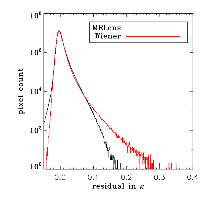
Figure 7: Histogram of the residual maps for Wiener and MRLens filtering.

A dedicated weak-lensing wavelet-restoration method, called MRLens, has been developed (Starck et al. 2006b). It can be considered to be an extension of the Maximum Entropy Method (MEM) that provides different types of information. In MRLens, the entropy constraint is not applied to the pixels of the solution, but rather its wavelet coefficients. This allows us to take into account more efficiently the multi-scale behavior of the information. MRLens was, however, designed for weak-lensing maps of smaller surface area on the sky, for which the non–Gaussian signal is stronger. MRLens was extended here to the sphere by considering independently each of the 12 Healpix base pixels covering the sphere as 12 independent Cartesian maps, on which we applied the MRLens algorithm of Starck et al. (2006b). Full-sky denoising performed with MRLens is shown in Fig. 5. It performs more efficiently than the Wiener methods on small scales, with dense clumps more accurately estimated, but less efficient than the Wiener method on large scale when recovering low frequency waves in the map. We also computed the angular power spectrum of the error map (see Fig. 4) in both cases (Wiener and MRLens). We can see that Wiener filtering outperforms MRLens on large scales. Interestingly, the MRLens errors decrease significantly above the transition scale we identified in the last section around $\ell\simeq 1000$ (see Fig. 4).

To compare both methods more quantitatively, we computed the skewness and kurtosis of both reconstructed maps. Results are shown in Fig. 6. We note that using map-making algorithms to recover the skewness and kurtosis of the true signal is not at all the optimal strategy: maximum likelihood estimators are more appropriate. We used high-order statistics here only to compare the relative merits of each method. It is striking to observe in Fig. 6 that the Wiener reconstructed map strongly underestimate the skewness and the kurtosis at small scale. This confirms quantitatively what was already visible in the maps (Fig. 5), namely that the Wiener method strongly suppresses high peaks in the map, affecting the tail of the probability distribution function. On the other hand, the MRLens reconstructed map has a significantly higher skewness and kurtosis than the original map: this wavelet–based method is only efficient in recovering high peaks in the signal, affecting the reconstructed probability density function in the opposite direction.

We now use the Probability Density Function (PDF) of the residual maps to compare each method (see Fig. 7). We confirm our visual impression from Fig. 5 that MRLens performs more efficiently than the Wiener method in recovering the high convergence, nonlinear features in the map. The positive high residual tail is reduced significantly by MRLens, as well as the dozen of strongly outlying pixels in the Wiener filterer map around $\kappa\simeq 0.35$ (see Fig. 7). MRLens, however, performs poorly for small values of the convergence ($\kappa\simeq\pm 0.05$), for which the PDF is well approximated by a Gaussian, an optimal situation for Wiener filtering.

The present analysis, based on using both the power spectrum of the residual maps and the high–order moments of the recovered map, strongly suggests that new methods should be developed using an hybrid, multi-resolution formulation; for instance, using spherical harmonics on large scales, while utilizing wavelets coefficients on small scales. The methodology of this combined approach could be based on the idea of Combined Filtering introduced by Starck et al. (2006a).

6 Conclusion

Using the 70 billion particles of the Horizon N–body Simulation, we have computed for the first time a realistic full-sky convergence map with a pixel resolution of $\Delta\theta\simeq 0.74$ arcmin². We have analyzed the resulting map using multi-resolution statistics (variance, skewness, and kurtosis) and angular power-spectrum analysis. We have shown that this simulated map spans 4 decades of useful signal in angular scale, with 2 decades within the linear, Gaussian regime and 2 decades well into the nonlinear, non–Gaussian regime. We have shown that, when considering a realistic sky cut, we can reliabily estimate high–order moments of the map above $\ell\simeq 200$. Using even higher resolution maps, angular scales smaller than $\theta\simeq 1^{{}^{\prime}}$ could be explored in future works, although the mass ditribution on these scales might be affected by baryons physics (Jing et al. 2006), so that the present map might already cover all cosmologically relevant scales.

As a first step towards a realistic map–making procedure, we have tested two de-noising schemes on a simplified fictitious dataset derived from the full-sky map, namely Wiener filtering and the MRLens method (Starck et al. 2006b). We have shown quantitatively that Wiener filtering is the most effective method on large scales, although some signal is lost on small scales. MRLens performs more effectively on small scales and recovers the dense clumps associated with dark matter halos, but deals less accurately with low frequency waves in the map. Hence, this work demonstrates the need for hybrid multi-resolution approach, e.g., by combining spherical harmonics and wavelet coefficients. The present analysis will be extended in future work to map–making algorithms dealing directly with galaxy shears. The simulated convergence map may prove to be an effective tool for the design of new map–making methods and for the preparation of the next generation weak–lensing surveys.

Appendix A Computing the convergence maps from simulations

We first recall how to compute the convergence in the Born approximation, and then present our new ray-tracing scheme.

A.1 Born approximation

We start by the formula relating the convergence to the density contrast:

$$\kappa(\hat{n})=\frac{3}{2}\Omega_{m}\int_{0}^{z_{s}}\frac{dz}{E(z)}\frac{\mathcal{D}(z)\mathcal{D}(z,z_{s})}{\mathcal{D}(z_{s})}\frac{1}{a(z)}\delta(\frac{c}{H_{0}}\mathcal{D}(z)\hat{n},z)\,,$$

which is valid for sources at a single redshift $z_{s}$, and $\mathcal{D}(z)=\frac{H_{0}}{c}\chi(z)$ is the dimensionless, comoving, radial coordinate ($d\mathcal{D}=dz/E(z)$). We now rewrite this formula in a form that is more suited to integration over redshift slices in a simulation:

$$\kappa(\theta_{pix})\approx\frac{3}{2}\Omega_{m}\sum_{b}W_{b}\frac{H_{0}}{c}\int_{\Delta z_{b}}\frac{cdz}{H_{0}E(z)}\delta(\frac{c}{H_{0}}\mathcal{D}(z)\hat{n}_{pix},z)\,,$$

where

$$W_{b}=\left(\int_{\Delta z_{b}}\frac{dz}{E(z)}\frac{\mathcal{D}(z)\mathcal{D}(z,z_{s})}{\mathcal{D}(z_{s})}\frac{1}{a(z)}\right)/\left(\int_{\Delta z_{b}}\frac{dz}{E(z)}\right)$$

is a slice-related weight, and the integral over the density contrast reads

$$I = \int_{\Delta z_{b}}\frac{cdz}{H_{0}E(z)}\delta(\frac{c}{H_{0}}\mathcal{D}(z)\hat{n}_{pix},z)\,,$$

$$= \int_{\Delta\chi_{b}}d\chi\delta(\chi\hat{n}_{pix},\chi)\,,$$

$$\approx \frac{V({\rm sim})}{N_{part}({\rm sim})}\left(\frac{N_{part}(\theta_{pix},z_{b})}{S_{pix}(z_{b})}-\Delta\chi_{b}\right)\,,$$

where

$$S_{pix}(z_{b})=\frac{4\pi}{N_{pix}}\frac{c^{2}}{H_{0}^{2}}\mathcal{D}^{2}(z_{b})$$

is the comoving surface of the spherical pixel. Interpreting all together, we obtain the following formula for the convergence map (omitting the $\Delta\chi_{b}$ term that corresponds to a constant term):

$$\kappa(\theta_{pix})=\frac{3\Omega_{m}}{2}\frac{N_{pix}}{4\pi}\left(\frac{H_{0}}{c}\right)^{3}\frac{V({\rm sim})}{N_{part}({\rm sim})}\sum_{b}W_{b}\frac{N_{part}(\theta_{pix},z_{b})}{\mathcal{D}^{2}(z_{b})}\,.$$ (1)

This is the equation used to derive the convergence map in the Born approximation.

A.2 Ray–tracig using multiple planes

We discuss here the formulae needed for the multi-plane computations, where we consider the lensing by a number of thin lenses located at $\{z_{b}\}$. We define

$$\kappa_{fac}=\frac{3}{2}\Omega_{m}\frac{N_{pix}}{4\pi}\left(\frac{H_{0}}{c}\right)^{3}\frac{V({\rm sim})}{N_{part}({\rm sim})}\,,$$

and

$$\zeta(z_{b},\theta)=\kappa_{fac}\omega(z_{b})\frac{N_{part}(\theta,z_{b})}{\mathcal{D}^{2}(z_{b})}\,,$$ (2)

with

$$\omega(z_{b})=\left(\int_{\Delta z_{b}}\frac{dz}{E(z)}\frac{\mathcal{D}(z)}{a(z)}\right)/\left(\int_{\Delta z_{b}}\frac{dz}{E(z)}\right)\,.$$

To follow the light rays, we are interested in computing the angular displacement field for each ray $i$ due to a slice at $z_{b}$. We then define

$$\alpha_{i}^{b}=\left(-2\nabla\Delta^{-1}\left(\zeta(z_{b})\right)\right)(\theta_{i})\,,$$ (3)

where the gradient and Laplacien are computed using angular covariant derivatives on the (unit) sphere, and $\theta_{i}$ is the current direction of light ray $i$ when it is incident on the slice $b$. Now, we start from light rays that are back-propagated from the observer at z=0 towards the source (here at z=1). We denote by $\{\theta^{1}\}$ the location of the Healpix centres, which corresponds to the initial directions of the back-propagated rays emanating from the observer. The tangent vectors to each light ray will be modified by the deflection field at each lens plane, defined by Eq.  3. Then, computing the displacement of the rays at slice $b$ reads

$$\@vec{\alpha}_{i}^{b}=\left(-2\nabla\Delta^{-1}(\zeta(z_{b})\right)(\theta_{i}^{b})\,.$$

We then update the direction $\@vec{\beta}_{i}^{b}$ of the rays according to the following rotation, $\cal R$:

$$\@vec{\beta}_{i}^{b}={\cal R}(\@vec{n}_{i}^{b}\times\@vec{\alpha}_{i}^{b},\|\@vec{\alpha}_{i}^{b}\|)\@vec{\beta}_{i}^{b-1}\,.$$ (4)

where $\@vec{\beta}_{i}^{0}=\@vec{n}_{i}^{1}$ (light rays emanate from the observer, thus in a direction perpendicular to the first slice), and $\@vec{n}_{i}^{b}$is the vector normal to slice $b$ at the intersection of light-ray $i$ on slice $b$. Equation (4) can be simplified by noting that $\@vec{\alpha}$ is expressed naturally in the local $(\@vec{e}_{\theta,}\@vec{e}_{\phi})$ basis of the tangent plane at position $(\theta,\phi)$:

$$\@vec{\alpha}=\|\@vec{\alpha}\|(\cos\delta\@vec{e}_{\theta}+\sin\delta\@vec{e}_{\phi})\,.$$

After calculating the new value of $\@vec{\beta}$, one needs to compute the intersection of the light rays with the next shell. We call $\@vec{x}_{i}^{b}$ the Cartesian position of the intersection of light ray $i$ with slice $b$, then the next intersection will be given by the solution for $\lambda$ of the system:

$$\@vec{x}_{i}^{b+1} = \@vec{x}_{i}^{b}+\lambda\@vec{\beta}_{i}^{b}$$

$$\lambda^{2}+2\lambda(\@vec{x}_{i}^{b}\cdot\@vec{\beta}_{i}^{b})+R_{b}^{2}-R_{b+1}^{2} = 0\,,\quad\lambda>0\,,$$

assuming that $\@vec{\beta}$ remains strictly unitary, and $R_{b}$ is the comoving radius of slice $b$. Once $\@vec{x}_{i}^{b+1}$ is known, it is easy to compute the new $\theta_{i}^{b+1}$ positions. The contributions to $\kappa$ are then calculated following Eq. 1, but where the slice contributions are interpolated at the displaced positions:

$$\kappa(\theta_{i=pix})=\frac{3}{2}\Omega_{m}\frac{N_{pix}}{4\pi}\left(\frac{H_{0}}{c}\right)^{3}\frac{V({\rm sim})}{N_{part}({\rm sim})}\sum_{b}W_{b}\frac{N_{part}(\theta_{i}^{b},z_{b})}{\mathcal{D}^{2}(z_{b})}\,.$$

We note that $\theta_{i}^{b}$ may fall into different pixels as a function of the slice $b$.

References

- Abrial et al. (2008) Abrial, P., Moudden, Y., Starck, J.-L., et al. 2008, Statistical Methodology, 5, 289
- Albrecht & Bernstein (2007) Albrecht, A. & Bernstein, G. 2007, Phys. Rev. D, 75, 103003
- Amara & Refregier (2006) Amara, A. & Refregier, A. 2006, ArXiv Astrophysics e-prints
- Bahcall & Soneira (1980) Bahcall, J. N. & Soneira, R. M. 1980, ApJS, 44, 73
- Basak et al. (2008) Basak, S., Prunet, S., & Benabed, K. 2008, Phys. Rev. D, 00, 00
- Benjamin et al. (2007) Benjamin, J., Heymans, C., Semboloni, E., et al. 2007, ArXiv Astrophysics e-prints
- Bertschinger (2001) Bertschinger, E. 2001, ApJS, 137, 1
- Colombi et al. (2008) Colombi, S., Novikov, D., Jaffe, A., & Pichon, C. 2008, MNRAS, 00, 00
- Das & Bode (2008) Das, S. & Bode, P. 2008, ApJ, 682, 1
- Eisenstein & Hu (1999) Eisenstein, D. J. & Hu, W. 1999, ApJ, 511, 5
- Fosalba et al. (2008) Fosalba, P., Gaztanaga, E., Castander, F., & Manera, M. 2008, MNRAS, 391, 435
- Fu et al. (2008) Fu, L., Semboloni, E., Hoekstra, H., et al. 2008, A&A, 479, 9
- Górski et al. (2005) Górski, K. M., Hivon, E., Banday, A. J., et al. 2005, ApJ, 622, 759
- Hamana et al. (2001) Hamana, T., Colombi, S., & Suto, Y. 2001, A&A, 367, 18
- Hoekstra (2003) Hoekstra, H. 2003, ArXiv Astrophysics e-prints
- Hu & Tegmark (1999) Hu, W. & Tegmark, M. 1999, ApJ, 514, L65
- Huterer (2002) Huterer, D. 2002, Phys. Rev. D, 65, 063001
- Jain & Seljak (1997) Jain, B. & Seljak, U. 1997, ApJ, 484, 560
- Jain et al. (2000) Jain, B., Seljak, U., & White, S. 2000, ApJ, 530, 547
- Jing et al. (2006) Jing, Y. P., Zhang, P., Lin, W. P., Gao, L., & Springel, V. 2006, ApJ, 640, L119
- Munshi et al. (2006) Munshi, D., Valageas, P., Van Waerbeke, L., & Heavens, A. 2006, ArXiv Astrophysics e-prints
- Pires et al. (2008) Pires, S., Starck, J. ., Amara, A., et al. 2008, ArXiv e-prints
- Prunet et al. (2008) Prunet, S., Pichon, C., Aubert, D., et al. 2008, ApJS, 178, 179
- Refregier (2003) Refregier, A. 2003, ARA&A, 41, 645
- Réfrégier et al. (2006) Réfrégier, A., Boulade, O., Mellier, Y., et al. 2006, in Presented at the Society of Photo-Optical Instrumentation Engineers (SPIE) Conference, Vol. 6265, Space Telescopes and Instrumentation I: Optical, Infrared, and Millimeter. Edited by Mather, John C.; MacEwen, Howard A.; de Graauw, Mattheus W. M.. Proceedings of the SPIE, Volume 6265, pp. 62651Y (2006).
- Spergel et al. (2007) Spergel, D. N., Bean, R., Doré, O., et al. 2007, ApJS, 170, 377
- Starck et al. (2006a) Starck, J.-L., Moudden, Y., Abrial, P., & Nguyen, M. 2006a, A&A, 446, 1191
- Starck et al. (2006b) Starck, J.-L., Pires, S., & Réfrégier, A. 2006b, A&A, 451, 1139
- Teyssier (2002) Teyssier, R. 2002, A&A, 385, 337
- Van Waerbeke et al. (2001) Van Waerbeke, L., Hamana, T., Scoccimarro, R., Colombi, S., & Bernardeau, F. 2001, MNRAS, 322, 918
- White & Vale (2004) White, M. & Vale, C. 2004, Astroparticle Physics, 22, 19