Magnetocapacitance in non-magnetic inhomogeneous media

Abstract

The dielectric response in a magnetic field is routinely used to probe the existence of coupled magnetic and elastic order in the multiferroics. However, here we demonstrate that magnetism is not necessary to produce a magnetocapacitance when the material is inhomogeneous. By considering a two-dimensional, two-component composite medium, we find a characteristic dielectric resonance that depends on magnetic field. We propose this as a possible signature of inhomogeneities and we argue that this behavior has already been observed in nanoporous silicon and some manganites.

The behavior of a material’s dielectric constant under an applied, alternating electric field provides a powerful probe of its microscopic properties. For example, dielectric relaxation (characterized by a delay in the electrical polarization with respect to the changing electric field) can signify the presence of non-interacting, freely-rotating dipoles Jonscher (1983). More recently, the dielectric response as a function of an applied static magnetic field has been used to determine whether or not a material is a multiferroic Hemberger et al. (2003); Kimura et al. (2003); Hur et al. (2004); Singh et al. (2005). In multiferroic systems, magnetic order and electrical polarization are coupled, thus giving rise to a magnetocapacitance. This magneto-electric coupling makes multiferroics a topic of interest owing to its potential application Eerenstein et al. (2005).

It is well known that Maxwell-Wagner extrinsic effects, such as inhomogeneities and contact effects, can enhance the dielectric constant and yield dielectric relaxation in the absence of intrinsic dipolar relaxation Maxwell (1991); Wagner (1913); Lunkenheimer et al. (2002). However, it was only recently appreciated that the Maxwell-Wagner effect can also yield a magnetocapacitance without multiferroicity and its associated magnetoelectric coupling, provided the material exhibits an intrinsic magnetoresistance Catalan (2006). Such effects clearly demonstrate that a magnetocapacitance is not sufficient to establish multiferroicity. On the other hand, having a magnetocapacitance without magnetoelectric coupling may be more practical for technological applications.

In this letter, we show that in an inhomogeneous medium one does not require even an intrinsic magnetoresistance to produce a magnetic-field-dependent dielectric constant. Thus, there is the possibility of a sizable magnetocapacitance without any magnetic order.

As far as we are aware, our work is the first to address the dielectric response of composite media in the presence of a magnetic field, in a regime relevant to semiconductors. While the dc magnetotransport in classical, disordered media has been studied extensively Isichenko (1992); Herring (1960); Dreizin and Dykhne (1973); Stroud and Pan (1976); Balagurov (1986); Parish and Littlewood (2003, 2005), there are very few works on the ac dielectric response. Moreover, the latter are restricted to metal-insulator composites which are either in the absence of a magnetic field Murtanto et al. (2006) or they have an electric-field frequency $\omega$ that is close to the plasma resonance frequency Bergman and Strelniker (1998). Such a regime is only applicable to highly metallic materials rather then the semiconducting compounds we are interested in here.

We find that the dielectric function of a composite medium exhibits unexpected behavior in a magnetic field and, as such, could be used as a probe for inhomogeneities. Specifically, we find a strong dielectric resonance as a function of frequency, where the position of the dissipation peak sensitively depends on magnetic field. Furthermore, the real part of the dielectric response even switches sign in the vicinity of the resonance at finite field. Using these results, we argue that inhomogeneities are a probable cause of the magnetic-field-dependent ‘dielectric relaxation’ observed in nanoporous silicon Vasic et al. (2007) and in some manganite compounds Rivas et al. (2006); Rairigh et al. (2007).

To focus our investigation, we restrict ourselves to a two-component, two-dimensional (2D) composite medium. This should be sufficient to describe the salient features of a disordered material, but simple enough for us to derive analytical expressions. We assume that the length scale of the inhomogeneities is much larger than all the microscopic length scales of the system, e.g. the mean free path. Thus, the local current density ${\mathbf{j}}(\omega,{\mathbf{r}})$ is related to the local electric field ${\mathbf{E}}(\omega,{\mathbf{r}})$ via Ohm’s law: ${\mathbf{j}}(\omega,{\mathbf{r}})=\hat{\sigma}(\omega,{\mathbf{r}}){\mathbf{E}}(\omega,{\mathbf{r}})\equiv i\omega\hat{\varepsilon}(\omega,{\mathbf{r}}){\mathbf{E}}(\omega,{\mathbf{r}})$, where $\hat{\sigma}(\omega,{\mathbf{r}})$ is the local conductivity tensor and $\hat{\varepsilon}(\omega,{\mathbf{r}})$ is the local dielectric function. Furthermore, we take the regime where (i) $1/\omega$ is much larger than the scattering time, and (ii) the intrinsic conductivity and dielectric constant of each component are frequency independent. Then, the conductivity tensor in a transverse magnetic field ${\mathbf{H}}=H\hat{z}$ is given by

$$\hat{\sigma}(\omega)=\frac{\sigma}{1+\beta^{2}}\left(\begin{array}[]{ccc}1&\beta&\\ -\beta&1&\end{array}\right)+i\omega\varepsilon\mathbf{1}$$ (3)

Here, $\sigma$ is the dc scalar conductivity, $\varepsilon$ is the bare dielectric constant and $\beta=\mu H$, where $\mu$ is the carrier mobility. In general, the quantities $\sigma$, $\varepsilon$ and $\mu$ will be random functions of space, but here we will only allow them to take on two different values.

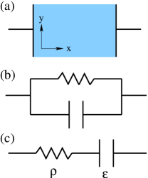
Figure 1: Simple circuits of resistors $\hat{\rho}\equiv\hat{\sigma}^{-1}$ and capacitors $\varepsilon$ that illustrate the basics of dielectric response. Diagram (a) depicts the measuring set-up, where a rectangular sample is confined between metallic plates and subjected to an applied electric field $E_{x}\hat{x}$, (b) represents a simple homogeneous medium, and (c) represents the simplest metal-insulator composite that exhibits the Maxwell-Wagner effect.

By taking volume averages over the composite medium, we can define an effective conductivity such that $\langle{\mathbf{j}}(\omega)\rangle=\hat{\sigma}_{e}(\omega)\langle{\mathbf{E}}(\omega)\rangle$. However, for the typical measuring set-up depicted in Fig. 1(a), we clearly have the boundary condition $j_{y}=0$, and so it is more natural to use the effective resistivity $\hat{\rho}_{e}(\omega)\equiv\hat{\sigma}_{e}(\omega)^{-1}$. Thus, the components of the dielectric function that are actually probed in experiment are given by $\varepsilon_{xx}(\omega)=(i\omega\rho_{e,xx}(\omega))^{-1}$ and $\varepsilon_{xy}(\omega)=(i\omega\rho_{e,xy}(\omega))^{-1}$. The longitudinal response $\varepsilon_{xx}(\omega)$ is simply the capacitance of the configuration in Fig. 1(a), while the transverse response $\varepsilon_{xy}(\omega)$ can be extracted from a measurement of the transverse electric field $E_{y}(\omega)=(\varepsilon_{xx}(\omega)/\varepsilon_{xy}(\omega))E_{x}(\omega)$. Note that in the limit $\beta\rightarrow 0$, we must have $E_{y}(\omega)\rightarrow 0$ and thus $\varepsilon_{xy}(\omega)\rightarrow\infty$.

First, it is instructive to consider a homogeneous medium described by the conductivity tensor in Eq. (3). One can represent this as a capacitor in parallel with a resistor (see Fig. 1(b)), where both circuit elements are frequency-independent. For this simple case, we find the real part of the longitudinal dielectric response to be

$$\Re[\varepsilon_{xx}(\omega)]=\frac{\varepsilon(1-\beta^{2}+(\omega\tau)^{2}(1+\beta^{2})^{2})}{1+(\omega\tau)^{2}(1+\beta^{2})^{2}}$$ (4)

where $\tau=\varepsilon/\sigma\equiv\rho\varepsilon$. Thus, we see that $\Re[\varepsilon_{xx}(\omega)]$ can be negative at sufficiently low frequencies when $\beta>1$. Usually, in the absence of a magnetic field, $\Re[\varepsilon_{xx}(\omega)]$ only goes negative at a dielectric resonance, and this signifies the presence of an inductive element in the system. However, for our simple resistor-capacitor circuit in a strong magnetic field, the boundary condition $j_{y}=0$ causes the Hall component of the resistive element to be mixed into the longitudinal dielectric response, resulting in a negative real part.

Now lets switch off the magnetic field and consider the simplest realization of an inhomogeneous medium: a resistor and capacitor in series (Fig. 1(c)). Here, we have dielectric function:

$$\varepsilon_{xx}(\omega) =\frac{\varepsilon(1-i\omega\tau)}{1+(\omega\tau)^{2}}$$ (5)

For low frequencies $\omega\tau<1$, the capacitor dominates the response, while at high frequencies $\omega\tau>1$, the voltage drop falls primarily over the resistor instead since there is insufficient time for the capacitor to build up charge. Thus, at the characteristic frequency $\omega\tau=1$, we have a rapid change in $\Re[\varepsilon_{xx}(\omega)]$ and an associated peak in $\Im[\varepsilon_{xx}(\omega)]$. This is a basic illustration of the Maxwell-Wagner effect, where the inhomogeneity mixes the real and imaginary modes of the response to create an apparent dielectric relaxation.

From these simple circuits, we see that geometric effects and macroscopic inhomogeneities can mix the different ‘modes’ (longitudinal, transverse, real and imaginary) of the system, and thus generate unexpectedly rich behavior, such as the dielectric resonance we will describe below. Inhomogeneities play a similar role in the dc magnetotransport of heavily disordered media, since they can mix the Hall resistivity into the longitudinal component to produce a linear magnetoresistance Parish and Littlewood (2003).

We now address the full problem of 2D isotropic inhomogeneous media. We suppose that the material is composed of two phases $\hat{\sigma}_{1}(\omega)$ and $\hat{\sigma}_{2}(\omega)$ in proportions $p_{1}=p$ and $p_{2}=1-p$, respectively. To model the dielectric response of a strongly inhomogeneous medium, we take the extreme case $\sigma_{1}=0$, $\varepsilon_{1}=\varepsilon$ and $\sigma_{2}=\sigma$, $\varepsilon_{2}=0$, i.e. we consider purely capacitive and purely resistive regions. When the proportions of each phase are equal ($p=1/2$), we can use a symmetry transformation for the current density and electric field Dykhne (1971); Balagurov (1978); Dykhne and Ruzin (1994) to derive the exact result for the components of the effective dielectric function:

$$\varepsilon_{xx}(\omega) =\varepsilon\frac{(1+i\omega\tau)}{\sqrt{i\omega\tau}\sqrt{(1+i\omega\tau)^{2}-(\omega\tau\beta)^{2}}}$$ (6)

$$\varepsilon_{xy}(\omega) =\frac{\varepsilon}{\beta}\left(1-\frac{i}{\omega\tau}\right)$$ (7)

We immediately see that the Hall component $\varepsilon_{xy}(\omega)$ is equivalent to the longitudinal dielectric response of a homogeneous material (Fig. 1(b)) in the absence of a magnetic field, with bare dielectric constant $\varepsilon/\beta$ and resistivity $\beta\rho$ (which is just the Hall resistivity for dc magnetotransport). As we will see below, this is unique to the case where the proportions are equal.

The longitudinal dielectric response $\varepsilon_{xx}(\omega)$, on the other hand, involves a non-trivial mixture of dielectric and resistive components in both the real and imaginary parts. The behavior is plotted in Fig. 2 and represents the key result of this paper. For large magnetic fields $\beta>1$, or, equivalently, for small frequencies $\omega\tau<1$, a dielectric resonance occurs at $\beta\omega\tau=1$, where $\Im[\varepsilon_{xx}(\omega)]$ has a pronounced peak and $\Re[\varepsilon_{xx}(\omega)]$ varies rapidly. In particular, we see that the resonant frequency is determined by the Hall resistivity $\beta\rho$, instead of $\rho$ like in the usual Maxwell-Wagner effect. Thus, the position of the peak in frequency space is inversely proportional to $\beta$. By substituting $\beta\omega\tau=1$ into Eq. (6), we see that the peak height $\Im[\varepsilon^{p}_{xx}]\simeq\varepsilon\beta/\sqrt{2}$. However, the actual dissipation at the peak remains constant because here we always have $\Re[\rho_{e,xx}]\simeq\sqrt{2}\rho$. In addition, the real part $\Re[\varepsilon_{xx}(\omega)]$ becomes negative for $\beta\omega\tau\gtrsim 1$ and $\beta>1$, but it exhibits ordinary Maxwell-Wagner dielectric relaxation at zero magnetic field. Surprisingly, there is no corresponding peak in $\Im[\varepsilon_{xx}(\omega)]$ when $\beta=0$, and this holds for arbitrary insulator fraction $p$ according to results obtained from the effective medium approximation and numerical resistor network studies Murtanto et al. (2006). This is particularly unexpected given that we obtain a dielectric relaxation peak from the simplest metal-insulator composite in Fig. 1(c). However, we speculate that one may recover the peak when the disorder is anisotropic since Fig. 1(c) is obviously highly anisotropic.

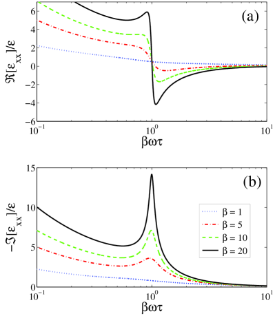
Figure 2: Dielectric response versus frequency over a range of magnetic fields $\beta$ for a 2D two-component medium with equal proportions ($p=1/2$). When $\beta>1$, there is a resonance at normalized frequency $\beta\omega\tau=1$, where the real part (a) varies rapidly, eventually changing sign, while the imaginary part (b) exhibits a peak.

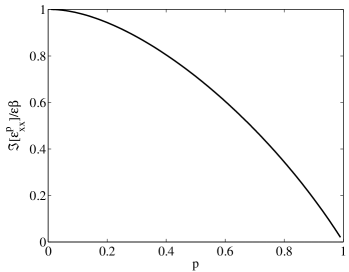
Figure 3: Behavior of the resonance peak $\Im[\varepsilon^{p}_{xx}]$ at $\beta\omega\tau=1$ as a function of the fraction $p$ of the insulating phase. This holds for all $\beta>1$.

To determine whether or not this dielectric resonance is a generic feature of 2D conductor-insulator composites, we use the effective medium approximation Stroud (1975); Guttal and Stroud (2005) to examine the case where $p\neq 1/2$. This amounts to numerically solving the coupled equations:

$$\sum_{i}p_{i}(\hat{\sigma}_{i}-\hat{\sigma}_{e})\left(\mathbf{1}-\frac{\hat{\sigma}_{i}-\hat{\sigma}_{e}}{2\sigma_{e,xx}}\right)^{-1} =0$$ (8)

When $\beta>1$, we find that there is always a resonance at $\beta\omega\tau=1$ for arbitrary $p$, but that the height of the dissipation peak $\Im[\varepsilon^{p}_{xx}(\omega)]$ decreases with increasing $p$ (decreasing conductor fraction) as shown in Fig. 3. Also, the behavior of $\Re[\varepsilon_{xx}(\omega)]$ is qualitatively unchanged at the resonance, apart from the fact that the point at which it switches sign occurs at a higher field for increasing $p$. This makes sense given that it is the Hall component of the conducting region that is responsible for the negative part of $\Re[\varepsilon_{xx}(\omega)]$.

The largest variation with respect to $p$ occurs in the Hall component $\Im[\varepsilon_{xy}(\omega)]$. As shown in Fig. 4, while $\Re[\rho/\rho_{e,xy}]$ is relatively insensitive to frequency for $p\leq 1/2$, it goes negative beyond a critical value of $\beta\omega\tau>1$ when $p>1/2$. Indeed, in the limit $p\rightarrow 1$, we have $\Re[\rho/\rho_{e,xy}]\rightarrow\infty$ for $\beta\omega\tau<1$ and $\Re[\rho/\rho_{e,xy}]\rightarrow-\infty$ for $\beta\omega\tau>1$, with $\Re[\rho/\rho_{e,xy}]=1/\beta$ always at $\beta\omega\tau=1$. Thus, we see there is some symmetry to the ‘mode-mixing’: the dielectric region reverses the sign of the Hall component at high frequencies in the same way that the Hall resistivity forces the dielectric constant to become negative at low frequencies. In principle, one could exploit this property to estimate the insulator fraction $p$ of a composite medium.

Figure 4: Hall component $\Re[\rho/\rho_{e,xy}]\equiv-\omega\tau\Im[\varepsilon_{xy}]/\varepsilon$ at $\beta=5$ as a function of frequency for different fractions $p$ of the insulating phase. Similar curves are obtained for other $\beta>1$. At $\beta\omega\tau=1$, $\Im[\varepsilon_{xy}]/\varepsilon=1$ for all $p$ and $\beta$.

Finally, we emphasize that the existence of the dielectric resonance is not conditional on there being a magnetoresistance at $\omega=0$. One clearly sees this from the fact that there is always a resonance at $\beta\omega\tau=1$ when $\beta>1$, even though the magnetoresistance is zero for $p<1/2$ and undefined for $p\geq 1/2$. One can obtain a non-zero magnetoresistance when the dielectric region has a non-zero conductivity $\sigma_{1}\neq\sigma_{2}$, but this saturates with magnetic field unless the proportions are equal ($p=1/2$) Guttal and Stroud (2005); Magier and Bergman (2006).

The magnetic-field-dependent dielectric resonance described above has already been observed experimentally in nanoporous silicon Vasic et al. (2007), a material which clearly resembles a conductor-insulator composite. Specifically, the dielectric response was measured as a function of temperature $T=25-40$K at fixed frequency $\omega=$ 100kHz and magnetic field $H=0-32$T, but this is equivalent to varying $\omega\tau$ if we assume that $\varepsilon$ is temperature-independent and that the electrical transport in the semiconductor is activated: $\rho=\rho_{0}e^{\Delta/k_{B}T}$, where $\Delta$ is the band gap. Then the temperature at which the resonance occurs is $k_{B}T=\Delta/\log(1/\beta\omega\varepsilon\rho_{0})$, so that we expect the dielectric resonance to shift to higher $T$ with increasing $H$, as indeed was observed. Assuming that $H=$ 1T corresponds to $\beta\simeq 1$, we can fit the data with $\Delta\simeq 30$meV and $\omega_{0}\equiv 1/\rho_{0}\varepsilon\simeq 8\times 10^{10}$Hz. Our results should be contrasted with an alternative proposal Brooks et al. which interprets the data with a model of Debye relaxation, requiring that charge carriers are pinned to a distribution of sites, but which does not explicitly introduce inhomogeneous fields.

In principle, one can exploit the dielectric resonance to construct a magnetic sensor that is sensitive to fields in the neighborhood of $\beta\sim 1/\omega\tau$. However, the challenge is to make it operational within the ideal frequency range $\omega=1$kHz$-1$MHz at room temperature and for $H<1$T, since this requires a semiconductor that has both a large band gap $\Delta>0.5$eV and a high mobility $\mu>1$T^-1.

A dielectric resonance has also been observed in the manganite La_2/3Ca_1/3MnO₃ at zero magnetic field, just above the ferromagnetic transition temperature Rivas et al. (2006). Moreover, Rairigh et al. Rairigh et al. (2007) observed a “colossal magnetocapacitance” coinciding with a regime of phase separation between magnetic metal and charge-ordered insulator. Magnetic materials have, of course, an intrinsic magneto-capacitive coupling, but we suggest that the magnetodielectric response is strongly enhanced in such a phase-separated composite, where the magnetized domains combine to produce a large internal magnetic field which acts on the transport currents.

To conclude, we have shown that a unique magnetic-field-dependent dielectric resonance is produced by a strongly inhomogeneous media and, as such, may be used as a probe of inhomogeneities or as a magnetic sensor.