Protecting Quantum Information with Entanglement and Noisy Optical Modes

Abstract

We incorporate active and passive quantum error-correcting techniques to protect a set of optical information modes of a continuous-variable quantum information system. Our method uses ancilla modes, entangled modes, and gauge modes (modes in a mixed state) to help correct errors on a set of information modes. A linear-optical encoding circuit consisting of offline squeezers, passive optical devices, feedforward control, conditional modulation, and homodyne measurements performs the encoding. The result is that we extend the entanglement-assisted operator stabilizer formalism for discrete variables to continuous-variable quantum information processing.

2007

LABEL:FirstPage1 LABEL:LastPage#1

I Introduction

Quantum computers and quantum communication systems will employ a variety of techniques to protect quantum information from the negative effects of decoherence Shor (1995); Steane (1996); Calderbank and Shor (1996); Gottesman (1997); Calderbank et al. (1997, 1998). Active quantum error-correcting techniques use multi-qubit measurements to learn about quantum errors and correct for these errors Zanardi and Rasetti (1997a, b); Lidar et al. (1998). Passive techniques exploit the symmetry of noisy quantum processes so that the quantum information we wish to protect remains invariant under the action of the noise Kribs et al. (2005, 2006); Poulin (2005); Brun et al. (2007); Hsieh et al. (2007).

We can classify the techniques according to the resources they employ for quantum redundancy: ancilla qubits, entangled qubits (ebits), or gauge qubits (qubits allowed to be noisy). A general technique for additive quantum error correction is the entanglement-assisted operator stabilizer formalism Brun et al. (2007); Hsieh et al. (2007)—it employs ancilla qubits, ebits, and gauge qubits for quantum redundancy. Figure 1 highlights the operation of an entanglement-assisted operator code.

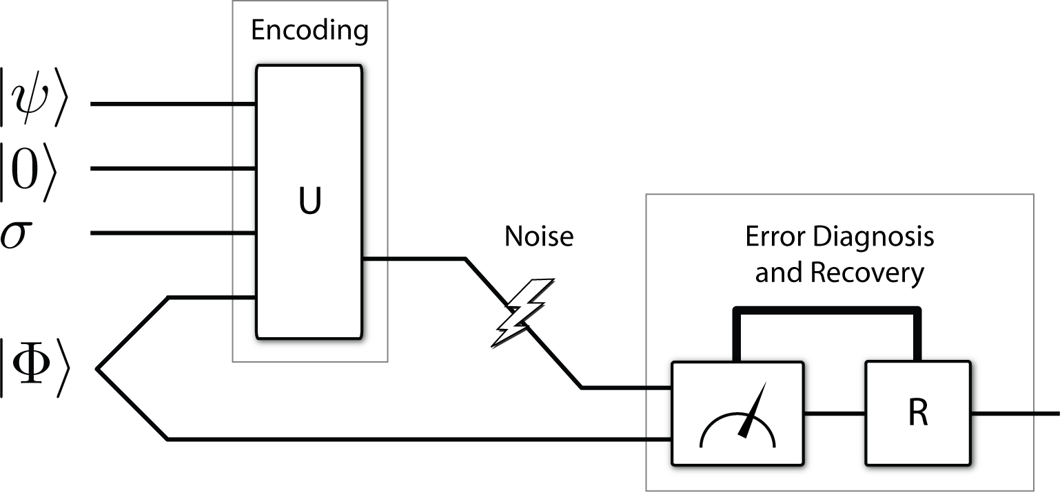
Figure 1: The operation of an $\left[\left[n,k;r,c\right]\right]$ entanglement-assisted operator quantum error-correcting code. The sender begins with a set of $k$ information qubits in state $\left|\psi\right\rangle$, $n-k-r-c$ ancilla qubits in state $\left|0\right\rangle$, $r$ gauge qubits in a mixed state $\sigma$, and $c$ ebits in state $\left|\Phi\right\rangle$. She encodes her information qubits with the help of the ancilla qubits, gauge qubits, and her half of the ebits. The receiver performs $n-k-r$ measurements on all of the qubits to diagnose errors. The $n-k-r$ measurements correspond to the $n-k-r$ ancilla qubits and ebits. The code also has passive error-correcting capability due to the use of ancilla qubits and gauge qubits.

Continuous-variable quantum information is an alternative to discrete-variable quantum information and has become increasingly popular for quantum computing and quantum communication Braunstein and Pati (2003); Braunstein and van Loock (2005). Experimentalists have performed many “proof-of-concept” experiments Furusawa et al. (1998); Mizuno et al. (2005); Li et al. (2002) that implement most of the basic protocols in continuous-variable quantum information theory Vaidman (1994); Braunstein and Kimble (1998); Ban (1999); Braunstein and Kimble (2000). Continuous-variable experiments are less difficult to perform than discrete-variable ones because they do not require single-photon sources and detectors and usually require linear optical devices only—offline squeezers, passive optical devices, feedforward control, conditional modulation, and homodyne measurements. An offline squeezer is a device that prepares a standard squeezed state for use in an optical circuit and an online squeezer is a nonlinear optical device used in an optical circuit. It is possible to simulate an online squeezer using a linear-optical circuit Filip et al. (2005). The recent proposal Filip et al. (2005) and experimental implementation of an online squeezer Yoshikawa et al. (2007a) and a quantum nondemolition interaction Yoshikawa et al. (2007b) using linear optics should further increase the popularity of continuous-variable quantum information processing. Several continuous-variable quantum protocols use this scheme Wilde et al. (2007b, c, a) and many more protocols should benefit from this technique.

Error correction is necessary for a continuous-variable quantum device to operate properly. Several authors have suggested methods for error correction of continuous-variable quantum information Braunstein (1998a); Lloyd and Slotine (1998); Braunstein (1998b); Wilde et al. (2007a); Niset et al. (2007). Some of these schemes Braunstein (1998a); Lloyd and Slotine (1998); Braunstein (1998b); Wilde et al. (2007a) are vulnerable to small displacement errors that occur in a continuous-variable quantum system Gottesman et al. (2001). They operate well only when the squeezing of optical parametric oscillators is high and the homodyne detectors are high efficiency. Experimentalists thus have a difficult technological challenge to overcome if continuous-variable quantum devices are to be practical. Nevertheless, these continuous-variable error correction schemes should prove useful as a testbed for theoretical ideas even if the final form of a quantum computer is not a continuous-variable optical device.

In this paper, we develop the entanglement-assisted operator stabilizer formalism for continuous-variable quantum systems. Our continuous-variable error correction scheme incorporates several forms of quantum redundancy: ancilla modes, entangled modes, and gauge modes. The benefit of our theory is that we can incorporate passive error-correction capability with a subsystem structure while still have the benefits of an entanglement-assisted code. Incorporating this subsystem structure may help in passively mitigating the effects of the small displacement errors that plague continuous-variable quantum systems.

We first briefly review the known techniques for discrete-variable quantum error correction. The next section discusses a canonical entanglement-assisted operator continuous-variable code and illustrate it with a quantum parity check matrix. We show how a local unitary relates an arbitrary entanglement-assisted operator code to the canonical one. Finally, we remark how a linear-optical circuit can perform the encoding operations using the techniques in Ref. Braunstein (2005) or Ref. Wilde et al. (2007a).

II Discrete-Variable Quantum Error Correction Techniques

We first review the different techniques for protecting discrete-variable quantum information. Each of the techniques falls into a class based on the resources it employs for quantum redundancy. Ancilla qubits provide both active and passive error-correcting capability, ebits provide active error-correcting capability, and gauge qubits provide passive error-correcting capability. A code is a subspace code if it uses only ancilla qubits or ebits, and it is a subsystem or operator code Knill et al. (2000) if it uses gauge qubits in addition to ancilla qubits or ebits. Stabilizer codes employ ancilla qubits only, operator codes employ ancilla qubits and gauge qubits, entanglement-assisted codes employ ancilla qubits and ebits, and entanglement-assisted operator codes employ ancilla qubits, ebits, and gauge qubits. We review each of the above methods in more detail below.

An $\left[\left[n,k\right]\right]$ stabilizer code corrects errors actively and passively by encoding $k$ information qubits with the help of $n-k$ ancilla qubits Gottesman (1997). The formalism operates in the Heisenberg picture by tracking a set of $n-k$ operators that stabilize the $k$ encoded information qubits. These $n-k$ operators equivalently correspond to logical Pauli $Z$ operators for the $n-k$ ancilla qubits. The receiver measures the $n-k$ operators corresponding to the encoded ancilla qubits to diagnose errors. These $n-k$ measurements learn only about quantum errors that occur and do not learn anything about the state of the $k$ information qubits. Stabilizer codes are active because they employ measurements to learn about the error and correct the encoded information qubits based on the result of the measurements. They are also passive because the $n-k$ operators corresponding to the ancilla qubits form a basis for errors that the code corrects passively.

Operator quantum error correction unifies active/passive stabilizer subspace coding techniques and passive subsystem techniques by respectively employing ancilla qubits and gauge qubits for quantum redundancy Kribs et al. (2005, 2006); Kribs and Spekkens (2006); Nielsen and Poulin (2007); Poulin (2005); Aly and Klappenecker (2008). An $\left[\left[n,k;r\right]\right]$ operator code encodes a set of $k$ information qubits with the help of $n-k-r$ ancilla qubits and $r$ gauge qubits. It operates similarly to a stabilizer code because the receiver measures the logical Pauli $\bar{Z}$ operators corresponding to the $n-k-r$ ancilla qubits to diagnose and correct some of the errors. The logical Pauli $\bar{X}$ and $\bar{Z}$ operators corresponding to the $r$ encoded gauge qubits form a basis for the errors that the code passively corrects. Operator codes have advantages over stabilizer codes to the degree that they might allow us reduce the number of measurements and corrections we have to perform to diagnose the error.

Entanglement-assisted codes correct errors both actively and passively by employing ancilla qubits and ebits for quantum redundancy Brun et al. (2006a, b, 2007); Hsieh et al. (2007); Wilde et al. (2007a). The technique assumes that a sender and receiver share pure noiseless entanglement (a set of ebits) prior to communication. An $\left[\left[n,k;c\right]\right]$ entanglement-assisted code encodes $k$ information qubits with the help of $n-k-c$ ancilla qubits and $c$ ebits. Methods exists to determine the optimal number of ebits that a given code requires Wilde and Brun (2008). The crucial assumption in the entanglement-assisted paradigm is that noise does not act on the receiver’s half of the ebits. The receiver measures the logical Pauli $\bar{Z}$ operators corresponding to the $n-k-c$ encoded ancilla qubits and the logical Pauli $\bar{X}^{A}X^{B}$ and $\bar{Z}^{A}Z^{B}$ operators corresponding to the $c$ encoded ebits to diagnose errors. Operators with an $A$ superscript correspond to Paulis acting on the sender’s side and those with a $B$ superscript correspond to a Pauli acting on the receiver’s side. A benefit of entanglement-assisted coding is that we can import any classical block or convolutional code for use in quantum error correction Brun et al. (2006b); Wilde et al. (2007d); Wilde and Brun (2007). Additionally, a source of pre-established entanglement boosts the rate of an entanglement-assisted code. We can produce an $\left[\left[n,k;c\right]\right]$ entanglement-assisted stabilizer code from an $\left[\left[n,k\right]\right]$ stabilizer code by replacing $c$ of the unencoded ancillas of the stabilizer code with $c$ ebits. The resulting entanglement-assisted code is more powerful than the original stabilizer code because it corrects a larger set of errors.

Entanglement-assisted operator quantum error correction combines the benefits of all of the above techniques by employing ancilla qubits, ebits, and gauge qubits for quantum redundancy Brun et al. (2007); Hsieh et al. (2007). An $\left[\left[n,k;c,r\right]\right]$ entanglement-assisted operator quantum error-correcting code encodes a set of $k$ information qubits with the help of $n-k-r-c$ ancilla qubits, $r$ gauge qubits, and $c$ ebits. This technique is the one of the most powerful known techniques for quantum error correction because it employs a large variety of resources for encoding.

III Continuous-Variable Mathematical Preliminaries

We review a few mathematical preliminaries that are necessary for continuous-variable quantum information processing before proceeding with our theory of error correction (See Ref. Wilde et al. (2007a) for a more detailed review.)

The displacement operators are the most important for continuous-variable quantum information processing. Let $X\left(x\right)$ denote a single-mode position-quadrature displacement by $x$ and let $Z\left(p\right)$ denote a single-mode momentum-quadrature “kick” by $p$ where

$$X\left(x\right) \equiv\exp\left\{-i\pi x\hat{p}\right\},$$

$$Z\left(p\right) \equiv\exp\left\{i\pi p\ \hat{x}\right\}.$$ (1)

Operators $\hat{x}$ and $\hat{p}$ are the position-quadrature and momentum-quadrature operators respectively with canonical commutation relations $\left[\hat{x},\hat{p}\right]=i$. We can extend the above definitions to multimode displacement operators with a map $\mathbf{D}$ as follows

$$\mathbf{D}\left(\mathbf{u}\right)\equiv\exp\left\{i\sqrt{\pi}{\textstyle\sum\limits_{i=1}^{n}}\left(p_{i}\hat{x}_{i}-x_{i}\hat{p}_{i}\right)\right\},$$ (2)

where $\mathbf{u}=\left(p_{1},\ldots,p_{n},x_{1},\ldots,x_{n}\right)\in\mathbb{R}^{2n}$ and the set of canonical operators $\hat{x}_{i},\hat{p}_{i}$ for all $i\in\left\{1,\ldots,n\right\}$ have the canonical commutation relations (in units where $\hbar=1$):

$$\left[\hat{x}_{i},\hat{x}_{j}\right] =0,$$

$$\left[\hat{p}_{i},\hat{p}_{j}\right] =0,$$

$$\left[\hat{x}_{i},\hat{p}_{j}\right] =i\delta_{ij}.$$

We also write $\mathbf{u}=\left(p_{1},\ldots,p_{n}\ |\ x_{1},\ldots,x_{n}\right)$ where the vertical bar separates the momentum-quadrature “kick” parameters from the position-quadrature displacement parameters. Let

$$\mathbf{X}\left(\mathbf{x}\right) \equiv X\left(x_{1}\right)\otimes\cdots\otimes X\left(x_{n}\right),$$

$$\mathbf{Z}\left(\mathbf{p}\right) \equiv Z\left(p_{1}\right)\otimes\cdots\otimes Z\left(p_{n}\right),$$ (3)

so that $\mathbf{D}\left(\mathbf{u}\right)$ and $\mathbf{Z}\left(\mathbf{p}\right)\mathbf{X}\left(\mathbf{x}\right)$ are equivalent up to a global phase. Another map $\mathbf{M}$ proves to be useful in our theory, where

$$\mathbf{M}\left(\mathbf{u}\right)\equiv\mathbf{u\cdot\hat{R}}^{n},$$ (4)

where $\mathbf{u}\in\mathbb{R}^{2n}$,

$$\mathbf{\hat{R}}^{n}=\left[\left.\begin{array}[c]{ccc}\hat{x}_{1}&\cdots&\hat{x}_{n}\end{array}\right|\begin{array}[c]{ccc}\hat{p}_{1}&\cdots&\hat{p}_{n}\end{array}\right]^{T},$$ (5)

and $\cdot$ is the inner product.

We can phrase continuous-variable quantum error correction theory in terms of the operators resulting from the maps $\mathbf{D}$ and $\mathbf{M}$ or in terms of the real vectors that result from the inverse maps $\mathbf{D}^{-1}$ and $\mathbf{M}^{-1}$. Both ways prove to be useful.

IV Canonical Entanglement-Assisted Operator Continuous-Variable Code

We begin our development of continuous-variable entanglement-assisted operator coding by introducing a canonical code. This canonical code actively and passively corrects for errors $\mathbf{D}\left(\mathbf{u}\right)$ in a canonical error set $S_{0}$ where $\mathbf{u}\in S_{0}\subset\mathbb{R}^{2n}$.

Suppose Alice wishes to protect a $k$-mode quantum state $\left|\psi\right\rangle$:

$$\left|\psi\right\rangle={\textstyle\idotsint}dx_{1}\cdots dx_{k}\ \psi\left(x_{1},\ldots,x_{k}\right)\ \left|x_{1}\right\rangle\cdots\left|x_{k}\right\rangle.$$ (6)

Alice and Bob possess $c$ sets of infinitely-squeezed, perfectly entangled states $\left|\Phi\right\rangle^{\otimes c}$ where

$$\left|\Phi\right\rangle\equiv\left(\int\ dx\ \left|x\right\rangle^{A}\left|x\right\rangle^{B}\right)/\sqrt{\pi}.$$ (7)

The state $\left|\Phi\right\rangle$ is a zero-valued eigenstate of the relative position observable $\hat{x}_{A}-\hat{x}_{B}$ and total momentum observable $\hat{p}_{A}+\hat{p}_{B}$. Alice possesses $l=n-k-c-r$ ancilla modes initialized to infinitely-squeezed zero-position eigenstates of the position observables $\hat{x}_{k+1},\ldots,\hat{x}_{k+l}$: $\left|\mathbf{0}\right\rangle=\left|0\right\rangle^{\otimes l}$. Alice also possesses an arbitrary mixed quantum state $\sigma$ over $r$ modes. These $r$ modes are the gauge modes. She encodes the state $\left|\psi\right\rangle$ with the canonical isometric encoder as follows:

$$U_{0}:\left|\psi\right\rangle\left\langle\psi\right|\rightarrow\left|\psi\right\rangle\left\langle\psi\right|\otimes\left|\mathbf{0}\right\rangle\left\langle\mathbf{0}\right|\otimes\sigma\otimes\left|\Phi\right\rangle\left\langle\Phi\right|.$$ (8)

The canonical encoder merely appends the $l$ ancilla modes, $r$ gauge modes, and $c$ entangled modes to the $k$ information modes.

Continuous-variable errors are equivalent to translations in position and kicks in momentum Braunstein (1998a); Gottesman et al. (2001). The canonical code corrects the error set

$$S_{0}=\left\{\begin{array}[c]{c}\left(\alpha\left(\mathbf{a},\mathbf{a}_{1},\mathbf{a}_{2}\right),\mathbf{b,\mathbf{c},a}_{2}|\beta\left(\mathbf{a},\mathbf{a}_{1},\mathbf{a}_{2}\right),\mathbf{a},\mathbf{d},\mathbf{a}_{1}\right)\\ :\mathbf{b,a}\in\mathbb{R}^{l},\ \ \mathbf{c,d}\in\mathbb{R}^{r},\ \ \mathbf{a}_{1}\mathbf{,a}_{2}\in\mathbb{R}^{c}\end{array}\right\},$$ (9)

for any known functions $\alpha,\beta:\mathbb{R}^{l}\times\mathbb{R}^{c}\times\mathbb{R}^{c}\rightarrow\mathbb{R}^{k}$. Consider an arbitrary error $\mathbf{D}\left(\mathbf{u}\right)$ where

$$\mathbf{u}=\left(\alpha\left(\mathbf{a},\mathbf{a}_{1},\mathbf{a}_{2}\right),\mathbf{b,\mathbf{c},a}_{2}|\beta\left(\mathbf{a},\mathbf{a}_{1},\mathbf{a}_{2}\right),\mathbf{a},\mathbf{d},\mathbf{a}_{1}\right).$$ (10)

Suppose an error $\mathbf{D}\left(\mathbf{u}\right)$ occurs. State $\left|\psi\right\rangle\left\langle\psi\right|\otimes\left|\mathbf{0}\right\rangle\left\langle\mathbf{0}\right|\otimes\sigma\otimes\left|\Phi\right\rangle\left\langle\Phi\right|$ becomes as follows (up to a global phase)

$$\mathbf{Z}\left(\alpha\right)\mathbf{X}\left(\beta\right)\left|\psi\right\rangle\left\langle\psi\right|\mathbf{X}\left(-\beta\right)\mathbf{Z}\left(-\alpha\right)\otimes\left|\mathbf{a}\right\rangle\left\langle\mathbf{a}\right|\otimes\sigma^{\prime}\otimes\\ \left|\mathbf{a}_{1},\mathbf{a}_{2}\right\rangle\left\langle\mathbf{a}_{1},\mathbf{a}_{2}\right|,$$ (11)

where $\left|\mathbf{a}\right\rangle=\mathbf{X}\left(\mathbf{a}\right)\left|\mathbf{0}\right\rangle$, $\left|\mathbf{a}_{1},\mathbf{a}_{2}\right\rangle=\mathbf{X}\left(\mathbf{a}_{1}\right)\mathbf{Z}\left(\mathbf{a}_{2}\right)\left|\Phi\right\rangle^{\otimes c}$, and

$$\sigma^{\prime}=\mathbf{Z}\left(\mathbf{c}\right)\mathbf{X}\left(\mathbf{d}\right)\sigma\mathbf{X}\left(-\mathbf{d}\right)\mathbf{Z}\left(-\mathbf{c}\right).$$ (12)

Bob measures the position observables of the ancillas $\left|\mathbf{a}\right\rangle$ and the relative position and total momentum observables of the state $\left|\mathbf{a}_{1},\mathbf{a}_{2}\right\rangle$. He obtains a reduced error syndrome $\mathbf{r}=\left(\mathbf{a,a}_{1},\mathbf{a}_{2}\right)$. The reduced error syndrome specifies the error up to an irrelevant value of $\mathbf{b}$, $\mathbf{c}$, and $\mathbf{d}$ in (10). The $\mathbf{b}$ errors are irrelevant because the ancilla modes absorb these errors (the ancillas are eigenstates of these error operators, and hence are unaffected by them.) The $\mathbf{c}$ and $\mathbf{d}$ errors are irrelevant because they affect the gauge modes only. Bob reverses the error $\mathbf{D}\left(\mathbf{u}\right)$ by applying the map $\mathbf{D}\left(-\mathbf{u}^{\prime}\right)$ where

$$\mathbf{u}^{\prime}=\left(\alpha\left(\mathbf{a},\mathbf{a}_{1},\mathbf{a}_{2}\right),\mathbf{0},\mathbf{0,a}_{2}|\beta\left(\mathbf{a},\mathbf{a}_{1},\mathbf{a}_{2}\right),\mathbf{a},\mathbf{0},\mathbf{a}_{1}\right).$$ (13)

This operation reverses the error because the states $\left|\psi\right\rangle\left\langle\psi\right|\otimes\sigma$ and $\left|\psi\right\rangle\left\langle\psi\right|\otimes\sigma^{\prime}$ differ by a gauge operation only and thus possess the same quantum information.

The canonical code is a simple example of a continuous-variable entanglement-assisted operator code, but it illustrates all of the principles that are at work in the operation of an entanglement-assisted operator code.

V Parity-Check Matrix for the Canonical Code

We now illustrate how the code operates in the Heisenberg picture by using a parity check matrix. A parity check matrix $F_{0}$ characterizes the operators that Bob measures:

$$F_{0} =\left[\left.\begin{array}[c]{ccccc}0&I&0&0&0\\ 0&0&0&I&-I\\ 0&0&0&0&0\end{array}\right|\begin{array}[c]{ccccc}0&0&0&0&0\\ 0&0&0&0&0\\ 0&0&0&I&I\end{array}\right]\begin{array}[c]{l}\}\ \ l\\ \}\ \ c\\ \}\ \ c\end{array}$$ (23)

$$=\left[\left.F_{Z0}\ \ \ \begin{array}[c]{c}0\\ -I\\ 0\end{array}\right|F_{X0}\ \ \ \begin{array}[c]{c}0\\ 0\\ I\end{array}\right]\begin{array}[c]{l}\}\ \ l\\ \}\ \ c\\ \}\ \ c\end{array},$$ (33)

where

$$F_{Z0}=\left[\begin{array}[c]{cccc}0&I&0&0\\ 0&0&0&I\\ 0&0&0&0\end{array}\right],\ \ F_{X0}=\left[\begin{array}[c]{cccc}0&0&0&0\\ 0&0&0&0\\ 0&0&0&I\end{array}\right].$$ (34)

These measurements diagnose errors on the modes that Alice sends over the noisy channel. The first column of zeros in $F_{Z0}$ and $F_{X0}$ has $k$ entries and corresponds to the $k$ information modes. The third column of zeros in $F_{Z0}$ and $F_{X0}$ has $r$ entries and corresponds to the $r$ gauge modes. The entries in $F_{Z0}$ and $F_{X0}$ correspond to the modes that Alice initially possesses and the last $c$ columns in $F_{0}$ to the right of $F_{Z0}$ and $F_{X0}$ correspond to the modes that Bob initially possesses. Noise does not affect these $c$ modes on Bob’s side because they are on the receiving end of the channel. The map $\mathbf{M}$ determines the observables that Bob measures to learn about the errors. Each row $\mathbf{f}$ of $F_{0}$ corresponds to an element of the set

$$\mathcal{M}_{0}\equiv\left\{\mathbf{M}\left(\mathbf{f}\right):\mathbf{f}\text{ is a row of }F_{0}\right\}.$$ (35)

Therefore, the first $l$ rows of $F_{0}$ correspond to the $l$ position observables and the last $2c$ rows of $F_{0}$ correspond to the relative position and total momentum observables. Matrix $F_{0}$ thus gives another way of describing the measurements performed in the canonical code. Bob measures the observables in $\mathcal{M}_{0}$ to learn about the error without disturbing the encoded state.

The following gauge matrix $G_{0}$ characterizes the errors that the code passively corrects due to the presence of gauge modes:

$$G_{0} =\left[\left.\begin{array}[c]{ccccc}0&0&I&0&0\\ 0&0&0&0&0\end{array}\right|\begin{array}[c]{ccccc}0&0&0&0&0\\ 0&0&I&0&0\end{array}\right]\begin{array}[c]{l}\}\ \ r\\ \}\ \ r\end{array}$$ (42)

$$=\left[\left.G_{Z0}\ \ \ \begin{array}[c]{c}0\\ 0\end{array}\right|G_{X0}\ \ \ \begin{array}[c]{c}0\\ 0\end{array}\right]\begin{array}[c]{l}\}\ \ r\\ \}\ \ r\end{array}.$$ (49)

The entries in $G_{0}$ form a basis for passively correctable errors. Therefore, the code passively corrects errors in the following set:

$$\mathcal{G}_{0}\equiv\left\{\mathbf{D}\left(\mathbf{g}\right):\mathbf{g}\in\text{rowspace}\left(G_{0}\right)\right\}.$$ (50)

This passive correction of errors is the additional benefit of including gauge modes in our codes. This incorporation of gauge modes may be able to help in correcting the small errors that plague continuous-variable quantum information systems.

The canonical code can correct an error set $\mathcal{E}_{0}$ that consists of all pairs of errors obeying the following condition: $\forall\ \mathbf{D}\left(\mathbf{e}\right),\mathbf{D}\left(\mathbf{e}^{\prime}\right)\in\mathcal{E}_{0}$ with $\mathbf{e}\neq\mathbf{e}^{\prime}$ either

$$\mathbf{e}-\mathbf{e}^{\prime}\notin\ \left(\text{rowspace}\left(F_{0,I}\right)\oplus\text{rowspace}\left(F_{0,E}\right)\right)^{\perp},$$ (51)

or

$$\mathbf{e}-\mathbf{e}^{\prime}\in\text{rowspace}\left(F_{0,I}\right)\oplus\text{rowspace}\left(G_{0}\right),$$ (52)

where

$$F_{0,I} =\left[\left.\begin{array}[c]{cccc}0&I&0&0\end{array}\right|\begin{array}[c]{cccc}0&0&0&0\end{array}\right],$$ (55)

$$F_{0,E} =\left[\left.\begin{array}[c]{cccc}0&0&0&I\\ 0&0&0&0\end{array}\right|\begin{array}[c]{cccc}0&0&0&0\\ 0&0&0&I\end{array}\right],$$ (60)

and $\perp$ denotes the symplectic dual Wilde et al. (2007a).

VI General Entanglement-Assisted Operator Codes

The relation between the canonical entanglement-assisted operator code and an arbitrary one is similar to the relation found in Ref. Wilde et al. (2007a). Alice can perform the encoding of an arbitrary code with a local unitary $U$. This local unitary $U$ preserves operators in the phase-free Heisenberg-Weyl group under conjugation Wilde et al. (2007a) and relates the canonical code to an arbitrary one. An equivalent representation of $U$ is with a symplectic matrix $\Upsilon$ that operates on the real vectors that result from the inverse maps $\mathbf{D}^{-1}$ and $\mathbf{M}^{-1}$. The former statement is equivalent to Theorem 2 from Ref. Wilde et al. (2007a).

A local unitary $U$ operating on the first $n$ modes relates the canonical code to a general one. In the Heisenberg picture, the symplectic matrix $\Upsilon$ is a $\left(2n\times 2n\right)$-dimensional matrix that takes the canonical parity check matrix $F_{0}$ to a general check matrix $F$ and the gauge matrix $G_{0}$ to a general gauge matrix $G$. The symplectic matrix $\Upsilon$ then performs the following transformation:

$$\left[\begin{array}[c]{cc}F_{Z0}&F_{X0}\end{array}\right]\Upsilon^{T} =\left[\begin{array}[c]{cc}F_{Z}&F_{X}\end{array}\right],$$ (63)

$$\left[\begin{array}[c]{cc}G_{Z0}&G_{X0}\end{array}\right]\Upsilon^{T} =\left[\begin{array}[c]{cc}G_{Z}&G_{X}\end{array}\right].$$ (66)

The parity check matrix $F$ for a general code has the following form:

$$F=\left[\left.F_{Z}\ \ \ \begin{array}[c]{c}0\\ -I\\ 0\end{array}\right|F_{X}\ \ \ \begin{array}[c]{c}0\\ 0\\ I\end{array}\right]\begin{array}[c]{l}\}\ \ l\\ \}\ \ c\\ \}\ \ c\end{array},$$ (67)

and the gauge matrix $G$ has the following form:

$$G=\left[\left.G_{Z}\ \ \ \begin{array}[c]{c}0\\ 0\end{array}\right|G_{X}\ \ \ \begin{array}[c]{c}0\\ 0\end{array}\right]\begin{array}[c]{l}\}\ \ r\\ \}\ \ r\end{array}.$$ (68)

Bob measures the observables in the set

$$\mathcal{M}\equiv\left\{\mathbf{M}\left(\mathbf{f}\right):\mathbf{f}\text{ is a row of }F\right\},$$ (69)

to diagnose and correct for errors. The code has passive protection against errors in the following set:

$$\mathcal{G}\equiv\left\{\mathbf{D}\left(\mathbf{g}\right):\mathbf{g}\in\text{rowspace}\left(G\right)\right\}.$$ (70)

The error-correcting conditions for our continuous-variable entanglement-assisted operator codes include those given in Ref. Wilde et al. (2007a). These codes also have some additional passive error-correcting capability due to the inclusion of gauge modes. Our codes can correct for all errors satisfying the conditions in Ref. Wilde et al. (2007a) and all errors $\mathbf{D}\left(\mathbf{u}\right)\in\mathcal{G}$. A general code can correct an error set $\mathcal{E}$ that consists of all pairs of errors obeying the following condition: $\forall\ \mathbf{D}\left(\mathbf{e}\right),\mathbf{D}\left(\mathbf{e}\right)^{\prime}\in\mathcal{E}$ with $\mathbf{e}\neq\mathbf{e}^{\prime}$ either

$$\mathbf{e}-\mathbf{e}^{\prime}\notin\ \left(\text{rowspace}\left(F_{I}\right)\oplus\text{rowspace}\left(F_{E}\right)\right)^{\perp},$$ (71)

or

$$\mathbf{e}-\mathbf{e}^{\prime}\in\text{rowspace}\left(F_{I}\right)\oplus\text{rowspace}\left(G\right),$$ (72)

where $F_{I}$ consists of the first $l$ rows of the matrix on the RHS of (63) and $F_{E}$ consists of the last $2c$ rows of the matrix on the RHS of (63) and $\perp$ denotes the symplectic dual Wilde et al. (2007a).

VII Example

We present an example of a continuous-variable entanglement-assisted operator code. This code is a straightforward extension of the entanglement-assisted Bacon-Shor code from Ref. Hsieh et al. (2007). We employ the method that Barnes suggested in Ref. Barnes (2004) that takes the stabilizer matrix for a discrete code and replaces “1” entries with a “1” or “–1” to make the symplectic product between rows be equal to one or zero. Our example encodes one information mode with the help of one set of entangled modes, four ancilla modes, and two gauge modes.

Its initial unencoded check matrix is as follows:

$$F_{0}=\left[\left.\begin{array}[c]{cccccccc}1&0&0&0&0&0&0&0\\ 0&1&0&0&0&0&0&0\\ 0&0&1&0&0&0&0&0\\ 0&0&0&1&0&0&0&0\\ 0&0&0&0&0&0&0&0\\ 0&0&0&0&1&0&0&0\end{array}\right|\begin{array}[c]{cccccccc}0&0&0&0&0&0&0&0\\ 0&0&0&0&0&0&0&0\\ 0&0&0&0&0&0&0&0\\ 0&0&0&0&0&0&0&0\\ 0&0&0&1&0&0&0&0\\ 0&0&0&0&0&0&0&0\end{array}\right].$$

Rows four and five of the above matrix correspond to half of an entangled mode and the other rows correspond to ancilla modes. The initial matrix for the gauge operators is as follows:

$$G_{0}=\left[\left.\begin{array}[c]{cccccccc}0&0&0&0&0&1&0&0\\ 0&0&0&0&0&0&0&0\\ 0&0&0&0&0&0&1&0\\ 0&0&0&0&0&0&0&0\end{array}\right|\begin{array}[c]{cccccccc}0&0&0&0&0&0&0&0\\ 0&0&0&0&0&1&0&0\\ 0&0&0&0&0&0&0&0\\ 0&0&0&0&0&0&1&0\end{array}\right].$$

The information mode corresponds to the last column of each of the above submatrices.

A linear-optical encoding operation (described in the next section) transforms the unencoded state to the encoded state. The check matrix corresponding to the encoded state is as follows:

$$F=\left[\begin{array}[c]{c}F_{Z}\end{array}\left|\begin{array}[c]{c}F_{X}\end{array}\right.\right],$$

where

$$F_{Z} =\left[\begin{array}[c]{cccccccc}1&-1&0&1&-1&0&0&0\\ 1&0&-1&1&0&-1&0&0\\ 0&0&0&0&0&0&1&-1\\ 0&0&0&0&0&0&0&0\\ 0&0&0&0&0&0&0&1\\ 0&0&0&0&0&0&0&0\end{array}\right],$$

$$F_{X} =\left[\begin{array}[c]{cccccccc}0&0&0&0&0&0&0&0\\ 0&0&0&0&0&0&0&0\\ 0&0&0&0&0&0&0&0\\ 1&1&1&0&0&0&-1&-1\\ 0&0&0&0&0&0&0&0\\ 1&1&1&-1&-1&-1&0&0\end{array}\right].$$

The matrix corresponding to the gauge operators is as follows:

$$G=\left[\left.\begin{array}[c]{cccccccc}0&0&0&0&0&0&0&0\\ 1&-1&0&0&0&0&0&0\\ 0&0&0&1&0&-1&0&0\\ 0&0&0&0&0&0&0&0\end{array}\right|\begin{array}[c]{cccccccc}0&1&0&0&-1&0&0&0\\ 0&0&0&0&0&0&0&0\\ 0&0&0&0&0&0&0&0\\ 0&0&1&0&0&-1&0&0\end{array}\right].$$

The code passively corrects error in the above gauge group. The receiver Bob measures the operators corresponding to rows one, two, three, and six in the matrix $F$. Bob combines his half of the entangled mode and measures operators corresponding to the following augmented version of rows four and five of $F$:

$$F_{\text{aug}}=\left[\left.\begin{array}[c]{cccccccc}0&0&0&0&0&0&0&0\\ 0&0&0&0&0&0&0&1\end{array}\begin{array}[c]{c}0\\ 1\end{array}\right|\begin{array}[c]{cccccccc}1&1&1&0&0&0&-1&-1\\ 0&0&0&0&0&0&0&0\end{array}\begin{array}[c]{c}1\\ 0\end{array}\right].$$

The code corrects an arbitrary single-mode error. This error-correcting capability follows directly from the discrete-variable code’s error-correcting properties.

VIII Encoding Circuit

Two different algorithms exist for constructing a linear-optical encoding circuit corresponding to the encoding unitary $U$ Braunstein (2005); Wilde et al. (2007a). The algorithm in Ref. Braunstein (2005) uses the Bloch-Messiah transformation to decompose a symplectic matrix into a sequence of passive optical transformations, online squeezers, and passive optical transformations. One can use the technique of Filip et al. for implementing the online squeezers. It is also possible to use the algorithm in Ref. Wilde et al. (2007a) for a linear-optical encoding circuit, but this technique uses quantum nondemolition interactions and may be more difficult to implement experimentally.

IX Concluding Remarks

Our EAQECCs are vulnerable to finite squeezing effects and inefficient photodetectors for the same reasons as those in Refs. Braunstein (1998a); Wilde et al. (2007a). Our scheme works well if the errors due to finite squeezing and inefficiencies in beamsplitters and photodetectors are smaller than the actual errors.

M.M.W. acknowledges support from NSF Grants CCF-0545845 and CCF-0448658, and T.A.B. acknowledges support from NSF Grant CCF-0448658.

References

- Shor (1995) P. W. Shor, Phys. Rev. A 52, R2493 (1995).
- Steane (1996) A. M. Steane, Phys. Rev. Lett. 77, 793 (1996).
- Calderbank and Shor (1996) A. R. Calderbank and P. W. Shor, Phys. Rev. A 54, 1098 (1996).
- Gottesman (1997) D. Gottesman, Ph.D. thesis, California Institue of Technology (1997).
- Calderbank et al. (1997) A. R. Calderbank, E. M. Rains, P. W. Shor, and N. J. A. Sloane, Phys. Rev. Lett. 78, 405 (1997).
- Calderbank et al. (1998) A. Calderbank, E. Rains, P. Shor, and N. Sloane, IEEE Trans. Inf. Theory 44, 1369 (1998).
- Zanardi and Rasetti (1997a) P. Zanardi and M. Rasetti, Phys. Rev. Lett. 79, 3306 (1997a).
- Zanardi and Rasetti (1997b) P. Zanardi and M. Rasetti, Mod. Phys. Lett. B 11, 1085 (1997b).
- Lidar et al. (1998) D. A. Lidar, I. L. Chuang, and K. B. Whaley, Phys. Rev. Lett. 81, 2594 (1998).
- Kribs et al. (2005) D. Kribs, R. Laflamme, and D. Poulin, Phys. Rev. Lett. 94, 180501 (2005).
- Kribs et al. (2006) D. W. Kribs, R. Laflamme, D. Poulin, and M. Lesosky, Quant. Inf. & Comp. 6, 383 (2006).
- Poulin (2005) D. Poulin, Phys. Rev. Lett. 95, 230504 (2005).
- Brun et al. (2007) T. Brun, I. Devetak, and M.-H. Hsieh, in IEEE International Symposium on Information Theory (2007), pp. 2101–2105.
- Hsieh et al. (2007) M.-H. Hsieh, I. Devetak, and T. Brun, Phys. Rev. A 76, 062313 (2007).
- Braunstein and Pati (2003) S. L. Braunstein and A. Pati, eds., Quantum Information with Continuous Variables (Springer, 2003).
- Braunstein and van Loock (2005) S. L. Braunstein and P. van Loock, Rev. Mod. Phys. 77, 513 (2005).
- Furusawa et al. (1998) A. Furusawa, J. L. S rensen, S. L. Braunstein, C. A. Fuchs, H. J. Kimble, and E. S. Polzik, Science 282, 706 (1998).
- Mizuno et al. (2005) J. Mizuno, K. Wakui, A. Furusawa, and M. Sasaki, Phys. Rev. A 71, 012304 (2005).
- Li et al. (2002) X. Li, Q. Pan, J. Jing, J. Zhang, C. Xie, and K. Peng, Phys. Rev. Lett. 88, 047904 (2002).
- Vaidman (1994) L. Vaidman, Phys. Rev. A 49, 1473 (1994).
- Braunstein and Kimble (1998) S. L. Braunstein and H. J. Kimble, Phys. Rev. Lett. 80, 869 (1998).
- Ban (1999) M. Ban, J. Opt. B: Quantum Semiclass. Opt. 1, L1 (1999).
- Braunstein and Kimble (2000) S. L. Braunstein and H. J. Kimble, Phys. Rev. A 61, 042302 (2000).
- Filip et al. (2005) R. Filip, P. Marek, and U. L. Andersen, Phys. Rev. A 71, 042308 (2005).
- Yoshikawa et al. (2007a) J.-I. Yoshikawa, T. Hayashi, T. Akiyama, N. Takei, A. Huck, U. L. Andersen, and A. Furusawa, arXiv:quant-ph/0702049 (2007a).
- Yoshikawa et al. (2007b) J. Yoshikawa, A. Huck, U. L. Andersen, and A. Furusawa, in Spring meeting of Physical Society of Japan, 19aXG-2 (2007b).
- Wilde et al. (2007a) M. M. Wilde, H. Krovi, and T. A. Brun, Phys. Rev. A 76, 052308 (2007a).
- Wilde et al. (2007b) M. M. Wilde, H. Krovi, and T. A. Brun, Phys. Rev. A 75, 060303 (2007b).
- Wilde et al. (2007c) M. M. Wilde, T. A. Brun, J. P. Dowling, and H. Lee, Phys. Rev. A 77, 022321 (2007c).
- Braunstein (1998a) S. L. Braunstein, Phys. Rev. Lett. 80, 4084 (1998a).
- Lloyd and Slotine (1998) S. Lloyd and J.-J. E. Slotine, Phys. Rev. Lett. 80, 4088 (1998).
- Braunstein (1998b) S. L. Braunstein, Nature 394, 47 (1998b).
- Niset et al. (2007) J. Niset, U. L. Andersen, and N. J. Cerf, arXiv:0710.4858 (2007).
- Gottesman et al. (2001) D. Gottesman, A. Kitaev, and J. Preskill, Phys. Rev. A 64, 012310 (2001).
- Braunstein (2005) S. L. Braunstein, Phys. Rev. A 71, 055801 (2005).
- Knill et al. (2000) E. Knill, R. Laflamme, and L. Viola, Phys. Rev. Lett. 84, 2525 (2000).
- Kribs and Spekkens (2006) D. W. Kribs and R. W. Spekkens, Phys. Rev. A 74, 042329 (2006).
- Nielsen and Poulin (2007) M. A. Nielsen and D. Poulin, Phys. Rev. A 75, 064304 (2007).
- Aly and Klappenecker (2008) S. A. Aly and A. Klappenecker, in Proceedings of the IEEE International Symposium on Information Theory (arXiv:0712.4321) (2008), pp. 369–373.
- Brun et al. (2006a) T. A. Brun, I. Devetak, and M.-H. Hsieh, arXiv:quant-ph/0608027 (2006a).
- Brun et al. (2006b) T. A. Brun, I. Devetak, and M.-H. Hsieh, Science 314, pp. 436 (2006b).
- Wilde and Brun (2008) M. M. Wilde and T. A. Brun, Phys. Rev. A 77, 064302 (2008).
- Wilde et al. (2007d) M. M. Wilde, H. Krovi, and T. A. Brun, arXiv:0708.3699 (2007d).
- Wilde and Brun (2007) M. M. Wilde and T. A. Brun, arXiv:0712.2223 (2007).
- Barnes (2004) R. Barnes, arXiv:quant-ph/0405064 (2004).