A note on artificial deformation in object shapes due to the pixelization

Abstract

We qualitatively examine properties of artificial deformation in shapes of objects (galaxies and stars) induced by the pixelization effects (also called as the aliasing effects) using toy mock simulation images. Two causes of the effects have been recognized: One is a consequence of observing the continuous sky with discrete pixels which is called as the first pixelization. And the other, called the second pixelization, is a consequence of resampling a pixelized image onto an another pixel grid whose coordinates are not perfectly adjusted to the input grid. We pay a special attention to the latter because it might be a potential source of a systematic noise in a weak lensing analysis. In particular, it is found that resampling with rotation induces artificial ellipticities in object shapes having a periodic concentric-circle-shaped pattern. Our major findings are as follows. (1) Root-mean-square (RMS) of artificial ellipticities in object shapes induced by the first pixelization effect can be as large as RMS$\gtrsim 10^{-2}$ if a characteristic size of objects (e.g., the FWHM) is smaller than twice of the pixel size. While for larger objects, it quickly becomes very small (RMS$\lesssim 10^{-5}$). (2) The amplitude of the shape deformation induced by the second pixelization effect depends on the object size. It also depends strongly on an interpolation scheme adopted to carry out resampling and on the grid size of the output pixels. The RMS of ellipticities in object shapes induced by the second pixelization effect can be suppressed to well below $10^{-2~{}}$ if one adopts a proper interpolation scheme (implemented in popular image processing softwares). We also discuss an impact of the pixelization effects on a weak lensing analysis.

1 Introduction

A precise shape measurement is of fundamental importance in astronomical research, not only because the morphology of celestial bodies provides us with their physical information, but also because tiny deformation in shapes of distant galaxies caused by gravitational lensing effect allows us to explore foreground mass distribution (see Fort & Mellier 1994; Mellier 1999; Bartelmann & Schneider 2001 for reviews). Analyses of weak gravitational lensing effect (e.g., the cosmic shear correlation) especially require very precise shape measurement, since its amplitude is of a few percents level (Refregier 2003 and references therein). Therefore, any artificial shape deformation which may arise during an observation as well as data reduction must be properly understood and must be controlled down to a sufficiently small level.

One known artificial shape deformation is caused by the pixelization of images, known as pixelization effects (also called as the aliasing effect). As pointed out by Rhodes et al. (2007), there are two causes of the pixelization effect (see Fig. 6 of Rhodes et al. 2007 for an illustration): One is a consequence of observing the continuous sky with discrete pixels, called as the first pixelization, which is an unavoidable effect. And the other, called as the second pixelization, occurs when resampling a pixelized image onto an another pixel grid whose coordinate is not perfectly adjusted to the input grid. During resampling, one input pixel may be resampled onto several output pixels, obviously resulting in deformation in object shapes (see Figure 2 for an illustration). The second pixelization occurs several stages of image processing processes involving resampling, for example, the correction for a geometric distortion, mosaicking images from multiple CCD chips to generate a combined image, and stacking multiple dithered images.

In this paper, we are concerned with the second pixelization effect taking two examples of resampling; rotation and correction for an axially symmetric optical distortion. We especially pay an attention to rotation which must be involved in the mosaic-stacking process of a mosaic CCD camera if multiple CCDs are not installed in perfectly parallel with each other. In the case of the Subaru Prime Focus Camera (Suprime-Cam), rotations of $0.025-0.17$ degrees are necessary for generating a properly mosaicked image. An important point to notice is that resampling with rotation induces artificial ellipticities in object shapes having a concentric-circle-shaped pattern (explained in detail in the following sections and see Figures 2 and 4 for demonstrations). Therefore it give rise to artificial shear correlations which can potentially act as a systematic noise in the measurement of cosmic shear correlation functions.

We notice that the artificial shape deformation induced by the second pixelization effect cannot be generally corrected by the anisotropic point spread function (PSF) correction (which is one of the important procedures in weak lensing analyses [Kaiser et al. 1995]) simply because they originate from different causes. The shape deformation by the anisotropic PSF arises during an observation with a real (thus non-perfect) instrument, thus it is an unavoidable effect and one has to develop a reliable correction scheme (e.g., Heymans et al. 2006; Massaey et al. 2007). Whereas the second pixelization effect occurs during image processing, and can be minimized by adopting an optimal resampling scheme. In fact, Rhodes et al (2007) developed such a resampling scheme for the HST ACS data in an empirical manner by searching for optimal parameters (the interpolation kernel and output pixel size) of the image processing software MultiDrizzle.

The purpose of this paper is two-fold: The first is to quantitatively examine the effect of the second pixelization effect to understand its properties. The second is to explore an optimum way to minimizing it. To do these, we use simple image simulations which is described in §2. Then in §3, we give some illustrative examples for a visual impression and for demonstrating the origin of the concentric-circle-shaped pattern induced by resampling with rotation. Results are presented in §4. Finally, §5 is devoted to a summary and discussion.

2 Simple image simulation

Since a very realistic mock simulation is not necessary for our purpose, we use a toy image simulation described below. We adopt two-dimensional Gaussian as a shape of “object”. The full-width-half-maximums (FWHM denoted by $\theta_{G}$) of the Gaussian object we consider are $\theta_{G}=0.4$, 0.6, 0.8, 1.2 and 2.0 arcsec. These object sizes are chosen because (i) the median seeing size (FWHM) of the Subaru telescope is about 0.6 arcsec and the best seeing is $\sim 0.35$ arcsec (Miyazaki et al. 2002), and (ii) most of objects used for weak lensing analyses are galaxies (and reference stars) with the FWHMs being smaller than 2 arcsec (Hamana et al. 2003).

We take the same pixel size as the Suprime-Cam, namely $\l_{\rm pixel}=0.2$ arcsec, as our primary science target is the weak lensing, especially using the Suprime-Cam or similar instruments. We create mock CCD images having $N_{x}\times N_{y}$ pixels on which Gaussian objects (having the equivalent FWHM and intensity) are located on a regular interval of $3\pi$ arcsec. Note that the separation between objects are more than 10 times of the $\sigma$ of the Gaussian ($\theta_{G}\simeq 2.35\times\sigma$), thus overlapping of isophotes of neighbour objects does not make any problem in the shape measurement. Note that results in this paper can be applied to any camera that uses a pixel array imaging device by properly translating the scaling ratio between $\theta_{G}$ and $l_{\rm pixel}$.

Figure 1: The RMSs of the ellipticities in object shapes caused by the first pixelization effect is plotted as a function of the FWHM of the Gaussian objects. Note that the RMS ellipticities of stars before the PSF correction is typically a few percents, and the RMS of intrinsic galaxy ellipticities is about 40 percents (e.g., Hamana et al. 2003).

Following the, so-called, KSB formalism (Kaiser, Squires & Broadhurst 1995), we quantify the image shapes by the ellipticity parameter defined by

$$\mbox{\boldmath$e$}=\left({{I_{11}-I_{22}}\over{I_{11}+I_{22}}},{{I_{12}}\over{I_{11}+I_{22}}}\right),$$ (1)

$$I_{ij}=\int d^{2}\theta~{}W_{G}(\theta)\theta_{i}\theta_{j}f(\mbox{\boldmath$\theta$}),$$ (2)

where $W_{G}(\theta)$ is the Gaussian window function. Notice that the $e_{1}$ ($e_{2}$) component represents the elongation in directions parallel (45 degrees rotated) to the coordinate system. The object detection and shape measurement are done with hfindpeaks and getshapes of IMCAT software suite developed by Nick Kaiser, respectively.

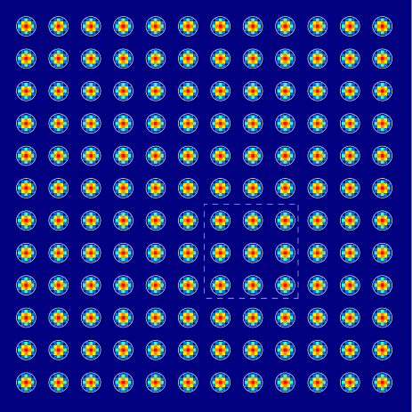
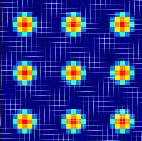
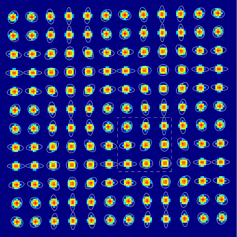
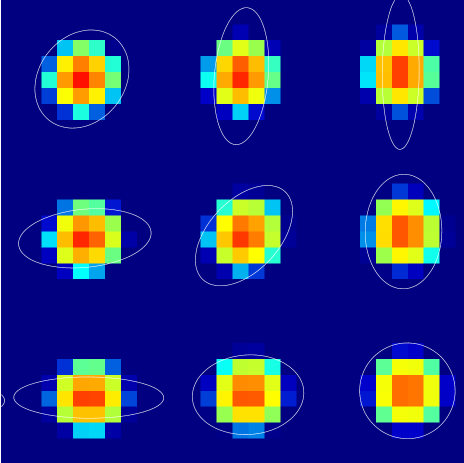
Figure 2: An illustrative example of the object shape deformations caused by the second pixelization. Top-left panel shows the simulation data of Gaussian objects with $\theta_{G}/l_{\rm pixel}=2$ located on a regular interval of 10 pixels. Note that the objects are placed just at the center of pixels to minimize the shape deformation caused by the first pixelization effect. The top-right panel shows the zoom-in on the section enclosed by the dashed line in the top-left panel. In this plot, a new grid (rotated by 1.15 degrees relative to the original grid) on which the image is resampled is over-plotted. The bottom two panels show the image after resampling onto the new grid. The resampling is done with the 1st order bilinear polynomial interpolation scheme. The over-plotted ellipses show the ellipticity of the objects. Note that the ellipticities are enlarged 10 times for clarify.

Before investigating the second pixelization effect, here we examine the first pixelization effect. The Gaussian has, of course, no ellipticity, but its pixelized image may have a finite ellipticity if the center of an object does not fall onto special positions such like the center of a pixel or an intersection of grid. We compute the root-mean-square (RMS) of the ellipticities among Gaussian objects in the simulation data of $2048\times 2048$ pixels. The RMS is defined by

$$\langle e^{2}\rangle^{1\over 2}=\left[\sum_{i=1}^{N_{obj}}(e_{i,1}^{2}+e_{i,2}^{2})/N_{obj}\right]^{1\over 2}.$$ (3)

Results are plotted in Figure 1. As expected, the RMS decreases with the object size. It quickly becomes large for smaller objects of $\theta_{G}<0.6$ arcsec and is $\sim 0.01$ for the case of $\theta_{G}=0.4$ arcsec ($\theta_{G}/l_{\rm pixel}=2$). This should be compared with the RMS ellipticities of stars (before the anisotropic PSF correction) which is typically a few percents. Thus if the seeing FWHM is less than twice of the pixel size, the first pixelization effect can be one of major sources of artificial shape deformation in small objects. An important finding here is that for objects with FWHM larger than three times the pixel size, the first pixelization effect is very small, but for smaller objects, the first pixelization effect can be a non-negligible source of the artificial ellipticities. Another point to be noticed here is that the pixelization effect does not necessarily generate the RMSs of $e_{1}$ and that of $e_{2}$ equally, because the pixels are square shaped and so the pixelization effect is, in general, not axially symmetric but has some special directions. This is the reason why the RMSs of two components are, in general, not equal as shown in Figure 1.

3 Visual impressions

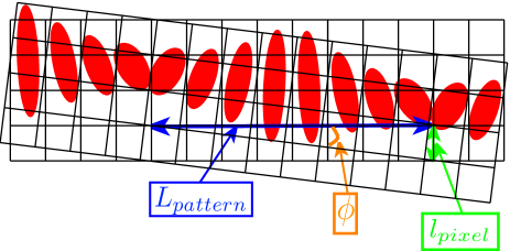
Figure 3: A sketch explaining the relation between the scale of the pattern ($L_{pattern}$), the pixel size ($l_{pixel}$) and the rotation angle ($\phi$). Two grids show the input and output grids which cross at an angle of $\phi$. The ellipses show the ellipticites (which are enlarged arbitrarily for clarify) of originally circular objects resampled onto the output grid. Notice that the same deformation pattern appears at the interval of $L_{pattern}$.

Before moving on to a thorough examination of the second pixelization effect, it would be helpful to present some illustrative examples of the second pixelization effect. Notice that in this section, for the illustrative purpose, we use simulation data which are different from ones used in §4 in the separation between objects. Figure 2 shows a demonstrative example for the origin of the periodic pattern caused by a resampling with a rotation. Here, we create simulation data of Gaussian objects with $\theta_{G}/l_{\rm pixel}=2$ located on a regular interval of 10 pixels. Note that the objects are placed exactly at the center of pixels to minimize the ellipticity induced by the first pixelization effect. The top-left panel shows the simulation image where ellipticities of object shapes are over-plotted by ellipses (circles in this case). The top-right panel shows the zoom-in on the section enclosed by the dashed line in the top-left panel. In this plot, a new grid (rotated 1.15 degrees relative to the original grid) on which the image is resampled is over-plotted. Note that the rotation angle of 1.15 degrees is much larger than a usual rotation angle involved in the mosaicking of multiple CCDs, but is chosen for the demonstrative purpose. The bottom two panels show the images after resampling onto the new pixels. It is evident from these plots that a periodic pattern of artificial ellipticities in object shapes are induced by the rotation. The characteristic scale of the pattern is written in terms of the pixel size and the rotation angle, $\phi$, as $L_{\rm pattern}=l_{\rm pixel}/\tan\phi$ ($\sim 50\times l_{\rm pixel}$ for $\phi=1.15$ degree). The reason of this is as follows (see Figure 3 for an illustration): The deformation is induced by the difference in the grid positions between the input and output grids. Thus if the difference in the grid positions is same at separate positions, the same deformation is induced at those positions. In $x$- and $y$-direction, the same difference in the grid positions occurs in the interval of $L_{\rm pattern}$, because it is the length that the output grid diagonally crosses (with the angle of $\phi$) the input grid by one pixel length. Thus $L_{\rm pattern}$ is the separation between positions (in $x$- and $y$-direction) where the same deformation is induced.

Next, in order to demonstrate the periodic patterns of ellipticities in object shapes appearing in realistic data, we create simulation data having the same dimensions as CCDs of Suprime-Cam (namely, $2048\times 4096$ pixels with $l_{\rm pixel}=0.2$ arcsec) on which Gaussian images of $\theta_{G}=0.6$ arcsec are placed on a regular interval of 20 arcsec. The data are rotated by 0.025, 0.075 or 0.15 degrees and are resampled onto new pixels by adopting the 1st order polynomial interpolation scheme (see §4 for details). These rotation angles are chosen because the actual rotation involved in mosaicking of the Suprime-Cam’s CCDs ranges from 0.025 to 0.17 degrees. Ellipticity maps of resampled images are shown in Figure 4, where the characteristic periodic patterns are clearly observed. The scales of the pattern are $L_{\rm pattern}=0.2^{\prime\prime}/\tan\phi\sim$ 7.6, 2.5 and 1.3 arcmin for $\phi=$ 0.025, 0.075 and 0.15 degrees, respectively. This explains, at least qualitatively, the origin of the concentric-circle-shaped pattern observed in the real data displayed in Figure 2 of Miyazaki et al. (2007). As evidently shown in Figure 4, the artificial ellipticities induced by the image rotation mostly lead to the E-mode shear. It is thus very important to note that in the presence of such systematic ellipticities, a smallness of the B-mode shear does not guarantee a successful correction of this systematic noise, and it may be difficult to distinguish this from signals arising from gravitational lensing. Thus it is necessary to develop a resampling procedure which suppresses the systematic to a sufficiently small level. This is exactly a purpose of this paper, and we explore the way to minimising the systematic in an empirical manner in the next section. Notice that the actual mosaick-stacking involves the rotation, displacement and enlargement/reduction of images, also a high order warping is operated to remove the optical distortion (e.g., see Miyazaki et al. 2007). Thus actual data may have more complex ellipticity pattern than ones found in the simple simulation in this section. In the next section, we shall qualitatively examine the second pixelization effect taking two realistic examples of resampling; namely rotation operated in mosaicking and correction for the optical distortion in the case of Suprime-Cam.

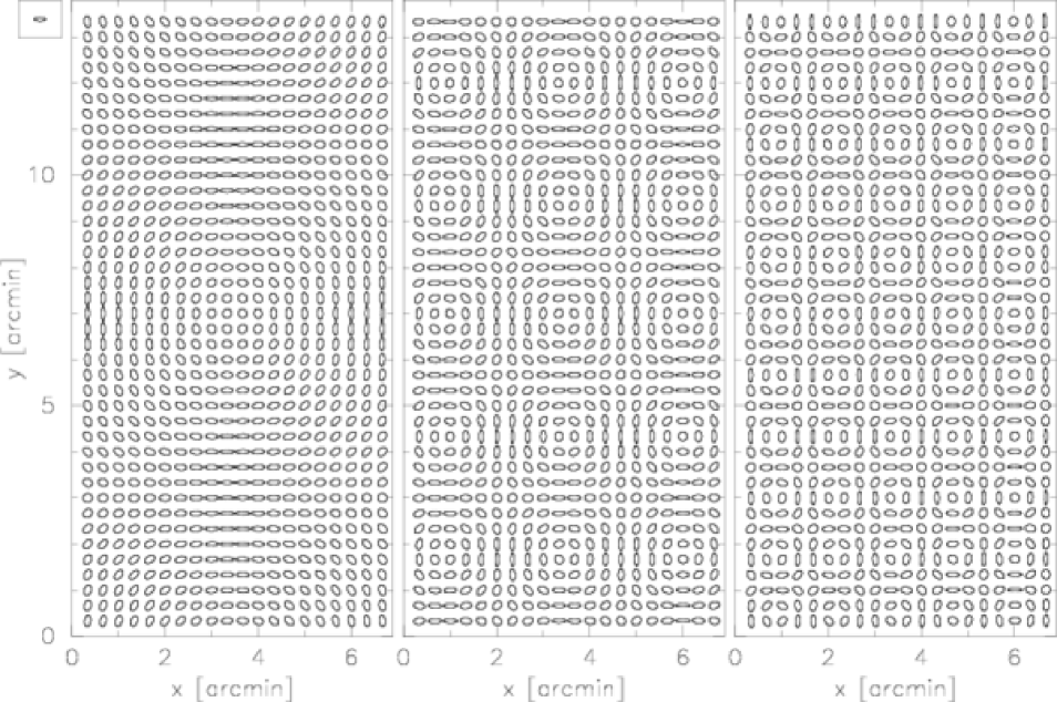
Figure 4: Ellipticity maps showing the periodic patterns of object shape deformations arising on realistic data. Simulation data having the same dimensions as CCDs of Suprime-Cam ($2048\times 4096$ pixels with $l_{\rm pixel}=0.2$ arcsec) on which Gaussian images of $\theta_{G}=0.6$ arcsec are placed on a regular interval of 20 arcsec, are rotated by 0.025, 0.075 and 0.15degrees (from left to right). Note that the ellipticities are enlarged 20 times for clarify. For comparison, an ellipse with $|e|=2\%$ (enlarged 20 times) is displayed in the small panel at the top-left corner.

4 Results

The magnitude of the second pixelization effect depends on the interpolation scheme used to resample an image. We examine the following interpolation schemes which are implemented in some popular image processing softwares: (i) the polynomial interpolation of 1st, 3rd and 5th order, for which we utilize transformimage of IMCAT. (ii) the sinc kernel [${\rm sinc}(x)=\sin(\pi x)/\pi x$] (truncated at 31 by 31 pixels), for which we utilize rotate of IRAF. (iii) Lanczos kernel [${\rm sinc}(x){\rm sinc}(x/a)$] of $a=2$, 3 and 4 (called Lanczos2, Lanczos3 and Lanczos4, respectively; implemented e.g., Swarp developed by Emmanuel Bertin), for which we utilize a resampling program developed by ourself. Also we examine the performance of adopting a finer grid for output pixels, which we call the grid refinement. Actually, it has been recognized that the grid refinement can reduce object shape deformation by the pixelization effects (Rhodes et al. 2007; Miyazaki et al. 2007) at the cost of the computational overheads. The grid refinement was tested in combination with the 1st and 3rd order polynomial interpolation schemes for which we utilize transformimage of IMCAT.

4.1 Rotation

The $2048\times 2048$ pixel simulation data described in §2 are rotated by 0.16 degrees and are resampled onto a new grid by applying one of the interpolation schemes mentioned above. The rotation angle of 0.16 degrees is chosen so that it is within the range of Suprime-Cam’s actual rotation angles in the mosaic-stacking procedure ($0.025-0.17$ degrees). Note that the RMS of the ellipticities after resampling does not depend on the rotation angle, though the size of the concentric-circle-shaped pattern does.

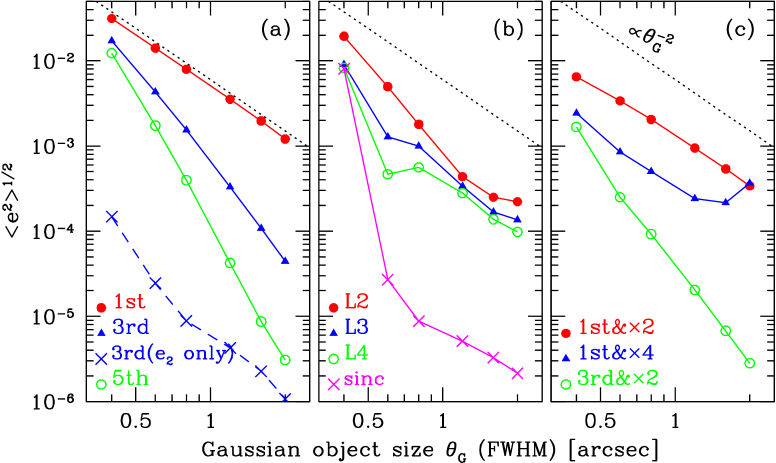
Figure 5: RMSs of ellipticitis in object shapes as a function of the object size are shown for comparison among various interpolation schemes. Left panel (a): the 1st, 3rd and 5th order polynomial for the filled circles, filled triangles and open circles respectively. The crosses show the contribution from $e_{2}$ component ($\langle{e_{2}}^{2}\rangle^{1/2}$) of the 3rd order polynomial, which demonstrates that the second pixelization effect mostly induces $e_{1}$ component. Middle panel (b): the Lanczos2, Lanczos3, Lanczos4 and sinc resampling schemes for the filled circles, filled triangles, open circles and crosses, respectively. Right panel (c): The 1st order polynomial with twice and 4 times finer grid for the filled circles and filled triangles respectively, and the 3rd order polynomial with twice finer grid for the open triangles.

Let us first look into the dependence of the second pixelization effect on the object size for various interpolation schemes. Figure 5 compares the RMSs of ellipticities in object shapes as a function of the object size. Left panel of Figure 5 compares the three polynomial interpolation schemes, revealing that the higher the order of polynomials is, the better performance one obtains. It is also found that the higher the order of polynomials is, the steeper the slope becomes. To be specific, the RMSs depend on the object size roughly, $\langle e^{2}\rangle^{1/2}\propto\theta_{G}^{-2}$ for the linear polynomial, and $\langle e^{2}\rangle^{1/2}\propto\theta_{G}^{-4}$ for the 3rd order, and further steeper slope for the 5th order. The crosses in the same plot show the RMS of $e_{2}$ component only for the case of the 3rd order polynomial, from which it is found that the $e_{2}$ component is much smaller than the total RMS. In fact, we found that the second pixelization effect preferentially induces $e_{1}$ component, irrespective of the interpolation schemes. This is due to the fact that the pixels are square shaped and so the pixelization effect has some special directions.

The middle panel of Figure 5 shows the results for the sinc and Lanczos kernels. It is found that the Lanczos2 works as well as the 3rd order polynomial does. The Lanczos3 and Lanczos4 are better than 3rd and 5th order polynomials for small objects ($\theta_{G}<0.6$ arcsec) but for larger objects ($\theta_{G}>1$ arcsec) they work only a little better than Lanczos2 does. The sinc kernel shows the best performance among the interpolation schemes (without the grid-refinement) we consider in this paper. We note that the sinc kernel is computationally expensive as it extends to very large area (e.g., 31 by 31 pixels for the default setting of IRAF).

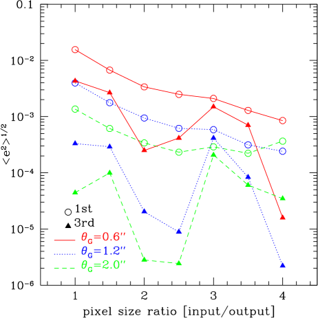
Figure 6: RMSs of ellipticitis in object shapes as a function of the ratio between the input and output pixel size. Open circles are for the linear polynomial interpolation scheme, while filled triangles are for the 3rd order polynomial. Different line styles are different object size: $\theta_{G}=0.6$, 1.2 and 2.0 for the solid, dotted and dashed line, respectively.

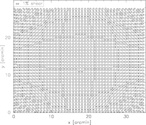
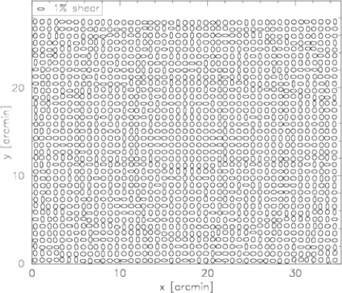
Figure 7: Ellipticity maps before (left) and after (right) the distortion correction. The left panel shows the mock simulation of the ellipticity map due to the optical distortion of the Suprima-Cam. The Gaussian objects with FWHM of 0.6 arcsec with the optical distortion are distributed on a mock Suprime-Cam pixels. The ellipses show the ellipticity of distorted Gaussian objects sparsely sampled from the mock simulation data (see §2). The right panel shows the ellipticity map of the distortion corrected data. For comparison, an ellipse with $|e|=1\%$ is displayed in the top-left corner.

Right panel of Figure 5 shows that the grid refinement nicely suppress the second pixelization effect. This is also observed in Figure 6 where the improvement gained by the grid refinement is plotted as a function of the ratio between input and output pixel size. If combined with the linear polynomial interpolation scheme, taking twice finer output grid reduces the RMSs by about one third with keeping the slope of $\langle e^{2}\rangle^{1/2}\propto\theta_{G}^{-2}$ mostly unchanged. The use of 4 times finer grid reduces the RMSs by about one order of magnitude for objects with $\theta_{G}<1.2$ arcsec and by lesser extent for larger objects. If combined with the 3rd order polynomial, improvements gained by the grid refinement behave irregularly as observed in Figure 6. Interestingly, in the case of an input/output pixel ratio of 3, adopting the 3rd order polynomial makes only a slight improvement over the 1st order case. An important message of this is that certain combinations may not give good improvement for the computational overhead, and thus care must be paid when one combines the grid refinement with a higher order interpolation scheme. Our experiment suggests that reasonably good improvement is stably obtained when one adopts the twice finer grid with the 3rd order polynomial interpolation.

4.2 Optical distortion

Next we examine the second pixelization effect induced during the correction for the optical distortion. To do so, we take the case for the Suprime-Cam. The optical distortion of the Suprime-Cam is axially symmetric with respect to the optical axis and is well approximated by the forth order polynomial function of the distance from the optical axis (see eq. [8] of Miyazaki et al. 2002). As is shown in Fig 21 of Miyazaki et al. (2002), the distortion rapidly increases with the distance from the optical axis.

Adopting the forth order polynomial model given in Miyazaki et al. (2002; their eq. [8]), we generate a mock Suprime-Cam images of $10456\times 8282$ pixels, on which Gaussian objects with $\theta_{G}=0.6$ arcsec with the optical distortion artificially operated, are distributed in the manner described in §2. In the left panel of Figure 7, the ellipticity map of the distorted Gaussian objects is shown. As is shown there, the Suprime-Cam’s optical distortion induces a radial elongation in the object shapes because the distortion becomes larger as the distance from the optical axis increases. The RMS of the ellipticities as a function of the distance from the optical axis is shown in Figure 8. At the central region where the distortion is smallest, the RMS ellipticity is as small as one induced by the first pixelization effect as expected. Whereas at the largest distance it becomes one percent. Note that in this case the first pixelization effect induces RMSs of $e_{1}$ and $e_{2}$ almost equally, and the turnover in $e_{1}$ component seen at $\theta\sim 17$ arcmin is an artifact due to the anisotropic sampling (objects in the largest distance are located only at the four corners, which preferentially have $e_{2}$ component as observed in Figure 8).

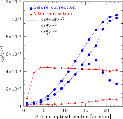
Figure 8: RMSs of ellipticitis in object shapes as a function of the distance from the optical axis. This is the result of the mock Gaussian simulation with the FWHM of 0.6 arcsec. Filled circles and filled triangles are for before and after distortion correction. The dotted and dashed lines are for $e_{1}$ and $e_{2}$ components, respectively, whereas the solid lines show the sum of them.

We correct for the optical distortion by resampling pixels with the 3rd order polynomial interpolation. The ellipticity map after the correction is shown in the right panel of Figure 7 from which one may visually realize that the radial deformation induced by the optical distortion is corrected successfully but artificial deformations due to the second pixlization effect appear. The important point recognized in the plot is that the ellipses are preferentially oriented to the directions parallel to the grids. This is quantitatively demonstrated in Figure 8 in which one may find that the RMS of the ellipticities after the correction almost solely comes from $e_{1}$ component. Note that the RMS only weakly depends on the the distance from the optical axis except for the most central region where the optical distortion is negligible and thus the correction is as well. The values of the RMS ( $\langle e^{2}\rangle^{1/2}\sim\langle{e_{1}}^{2}\rangle^{1/2}\sim 4\times 10^{-3}$ and $\langle{e_{2}}^{2}\rangle^{1/2}\sim 5\times 10^{-4}$) are equivalent to that found in the case of the rotation (Figure 5). These similarities suggest that the RMS ellipticities induced by the second pixelization effect does not depend on resampling parameters (e.g., displacements, rotation and anisotropic transformation) but solely depends on the ratio between the object size and the pixel size. Although this could be a specific feature of the Gaussian, it might be generally said that the magnitude of the second pixelization effect most strongly depends on the object size.

Notice that in a closer look at the left panel of Figure 7 one may observe partially mirror symmetric patterns with respect to the $x$- and $y$-axis passing through the field center. The reason of this is that although the optical distortion and thus the correction for it are axially symmetric, resampling onto square pixels does not induce an axially symmetric pattern but results in the partially mirror symmetric pattern. Except for it, we do not observe any obvious characteristic pattern.

5 Summary and Discussions

We have qualitatively examined ellipticities in object shapes induced by the pixelization effects paying a special attention to the periodic concentric-circle-shaped pattern induced by resampling of pixels with rotation. Our major findings are summarized as follows.

• Artificial ellipticities induced by the first pixelization effect can be as large as $\langle e^{2}\rangle^{1/2}\gtrsim 10^{-2}$ if a characteristic size of objects (e.g., the FWHM) is smaller than twice of the pixel size. Whereas for objects with the characteristic size being larger than three times of the pixel size, the RMS becomes negligibly small ($\langle e^{2}\rangle^{1/2}\lesssim 10^{-5}$).

• The second pixelization effect preferentially induces the $e_{1}$ component (parallel to the grids). The reason of this is that pixels are square shaped and so the pixelization effect is, in general, not axially symmetric but has some special directions.

• The size (e.g., RMS of $e$) of the shape deformation caused by the second pixelization effect depends on the object size. It also strongly depends on the interpolation scheme for resampling and on the grid size of the output pixels. If we set an upper limit of the RMS ellipticies by $\langle e^{2}\rangle^{1/2}<5\times 10^{-3}$ for objects with FWHM$>2.5\times l_{\rm pixel}$ (corresponding to FWHM$>0.5$ arcsec for the case of Suprime-Cam), the interpolation schemes passing the above condition are (see Figure 5) the 5th order polynomial, Lanczos3, Lanczos4 and sinc kernel (as far as among ones considered in this paper). Adopting the grid refinement makes a great improvement. Actually, if one adopts twice finer grid for output pixels, even the linear polynomial can pass the above condition.

• Resampling of a pixelized image with rotation induces a periodic concentric-circle-shaped pattern of artificial ellipticities in object shapes. The scale of the pattern is related to the pixel size and the rotation angle, $\phi$, by $L_{\rm pattern}=l_{\rm pixel}/\tan\phi$.

Before closing this paper, we would like to make a comment on an impact of the second pixelization effect on the actual weak lensing analysis using Suprime-cam data presented in Miyazaki et al. (2007). Miyazaki et al. (2007) carried out resampling adopting the 3rd order polynomial interpolation scheme and combined typically 4 dithered images, thus for the images with FWHM$\gtrsim 0.6$ arcsec (the typical PSF size), the RMS of ellipticities induced by the second pixelization effect should be well below $10^{-2}$. Whereas, the RMSs measured from stellar images are about a few $\times 10^{-2}$, therefore we may safely conclude that the second pixelization effect is suppressed sufficiently, and is not a major source of the artificial ellipticities in object shapes.

We would like to thank Richard Massey for valuable comments and Nick Kaiser for making the IMCAT software available. We would like to thank the anonymous referee for valuable and constructive comments on the earlier manuscript which improve the paper. This research was supported in part by the Grants–in–Aid from Monbu–Kagakusho and Japan Society of Promotion of Science (15340065 and 17740116). Numerical computations presented in this paper were carried out on computer system at CfCA (Center for Computational Astrophysics) and at ADAC (Astronomical Data Analysis Center) of the National Astronomical Observatory Japan.

References

- [BS(2001)] Bartelmann M., Schneider P. 2001, Phys. Rep., 340, 291
- [FM(1994)] Fort, B., Mellier, Y. 1994, A&AR, 5, 239
- [Hamana et al (2003)] Hamana, T., Miyazaki, S., Shimasaku, K., Furusawa, H., Doi, M., Hamabe, M., Imi, K., Kimura, M., Komiyama, Y., Nakata, F., Okada, N., Okamura, S., Ouchi, M., Sekiguchi, M., Yagi, M., Yasuda, N. 2003, ApJ, 597, 98
- [STEP1 (2006)] Heymans, C. et al. 2006, MNRAS, 368, 1323
- [Kaiser et al.(1995)] Kaiser, N., Squires, G., Broadhurst, T. 1995, ApJ, 449, 460
- [STEP2 (2007)] Massey, R. et al. 2007, MNRAS, 376, 13
- [Mellier(1999)] Mellier, Y. 1999, ARA&A, 37, 127
- [Suprime-Cam(2002)] Miyazaki, S., Komiyama, Y., Sekiguchi, M., Okamura, S., Doi, M., Furusawa, H., Hamabe, M., Imi, K., Kimura, M., Nakata, F., Okada, N., Ouchi, M., Shimasaku, K., Yagi, M., Yasuda, Naoki. 2002, PASJ, 54, 833
- [Suprime-Cam(2007)] Miyazaki, S., Hamana, T., Ellis, R. S., Kashikawa, N., Massey, R. J., Refregier, A. 2007, ApJ, 669, 714
- [Refregier(2003)] Refregier, A. 2003, ARA&A, 41, 645
- [Rhodes et al(2007)] Rhodes, D. J., Massey, R., Albert, J., Collins, N., Ellis, R. S., Heymans, C., Gardner, J. P., Kneib, J-P., Koekemoer, A., Leauthaud, A., Mellier, Y., Refregier, A., Taylor, J. E., Van Waerbeke, L. 2007, ApJS, 172, 203