Kondo effect in carbon nanotube quantum dots with spin-orbit coupling

Abstract

Motivated by recent experimental observation of spin-orbit coupling in carbon nanotube quantum dots [F. Kuemmeth et al., Nature (London) 452, 448 (2008)], we investigate in detail its influence on the Kondo effect. The spin-orbit coupling intrinsically lifts out the fourfold degeneracy of a single electron in the dot, thereby breaking the $SU(4)$ symmetry and splitting the Kondo resonance even at zero magnetic field. When the field is applied, the Kondo resonance further splits and exhibits fine multipeak structures resulting from the interplay of spin-orbit coupling and Zeeman effect. Microscopic cotunneling process for each peak can be uniquely identified. Finally, a purely orbital Kondo effect in the two-electron regime is also predicted.

Introduction.—The Kondo effect is one of the most fascinating and extensively studied subjects in condensed matter physics book1 . Since its first experimental observation in semiconductor quantum dots (QDs) in 1998 Goldhaber-Gordon , after 10 years of theoretical predictions Ng1988 , various aspects of this effect have been explored in virtue of the tunability of relevant parameters in the QDs. The Kondo physics was further enriched by fabricating carbon nanotube (CNT) QDs Nygard ; Buitelaar ; Jarillo-Herrero1 ; Jarillo-Herrero2 ; Makarovski1 ; Makarovski2 where additional orbital degree of freedom originating from two electronic subbands can play a role of pseudospin. In CNT QDs, spin-orbit coupling is widely believed to be weak and two sets of spin-degenerate orbits are expected to yield a fourfold-degenerate energy spectrum which possesses an $SU(4)$ symmetry. Consecutive filling of these orbits forms four-electron shells Buitelaar ; Jarillo-Herrero1 ; Jarillo-Herrero2 ; Makarovski1 ; Makarovski2 ; Liang . In each shell, the $SU(4)$ Kondo effect was observed in the valleys with one, two, and three electrons Jarillo-Herrero1 ; Jarillo-Herrero2 ; Makarovski1 ; Makarovski2 . Theoretically, the $SU(4)$ Kondo effect in CNT QDs has also been extensively studied Choi ; Lim ; Busser ; Anders

However, recent theories Huertas-Hernando2006 suggest that spin-orbit interaction can be significant in CNTs due to their curvature and cylindrical topology. More recently, transport spectroscopy measurements on ultra-clean CNT QDs by Kuemmeth et al. Kuemmeth demonstrate that the spin and orbital motion of electrons are strongly coupled, thereby breaking the $SU(4)$ symmetry of electronic states in such systems. This motivates us to reconsider the Kondo effect in CNT QDs by explicitly taking account of the spin-orbit coupling since this symmetry-breaking perturbation at the fixed point must break the $SU(4)$ Kondo effect studied previously. An important consequence is that even at zero magnetic field the Kondo effect manifests as split resonant peaks in the differential conductance. At finite fields, these peaks further split into much complicated subpeaks, reflecting the entangled interplay of spin and orbital degrees of freedom. Concerning all microscopic cotunneling events involving spin and/or orbit flip, these fine multipeak structures can be uniquely identified. Moreover, the spin-orbit coupling also determines the filling order in the two-electron ($2e$) ground state Kuemmeth , producing a purely orbital Kondo effect different from that observed by Jarillo-Herrero et al. Jarillo-Herrero1 .

Model Hamiltonian and QD Green’s function.—We model a CNT QD coupled to source and drain leads by the Anderson Hamiltonian $H=H_{d}+H_{L}+H_{T}$, where $H_{d}=\sum_{m}\varepsilon_{m}d_{m}^{\dagger}d_{m}+\frac{U}{2}\sum_{m\neq m^{\prime}}\hat{n}_{m}\hat{n}_{m^{\prime}}$, $H_{L}=\sum_{k,m,\alpha}\varepsilon_{k}C_{km\alpha}^{\dagger}C_{km\alpha}$, $H_{T}=\sum_{k,m,\alpha}V_{\alpha}d_{m}^{\dagger}C_{km\alpha}+\textrm{H.c.}.$ $H_{d}$ models the isolated CNT QD with $\hat{n}_{m}=d_{m}^{\dagger}d_{m}$. $d^{\dagger}_{m}$ ($d_{m}$) creates (annihilates) an $m=\{\sigma,\,\lambda\}$ configuration electron in the dot, where $\sigma,\lambda=\pm$ are the spin and orbital quantum numbers, respectively. $U$ denotes the on-site Coulomb repulsion, and $\varepsilon_{m}$ is the single-particle energy. $H_{L}$ models the two leads ($\alpha=L,R$). The tunneling between the dot and the leads is described by $H_{T}$ with spin and orbital conservation since the dot and the leads are usually fabricated within a same CNT and thus have the same orbital symmetry Jarillo-Herrero1 ; Jarillo-Herrero2 ; Makarovski1 ; Makarovski2 . Assuming some orbital mixing, a crossover from $SU(4)$ to $SU(2)$ Kondo effect has been investigated Choi ; Lim . Here we focus on a totally different breaking of the $SU(4)$ Kondo effect by the spin-orbit interaction which intrinsically lifts out the degeneracy in the single-particle energy.

The energy spectrum of CNT QDs in low-energy limit is $\varepsilon_{k}\simeq\hbar v_{F}\left|k\right|$ with $v_{F}$ the Fermi velocity and $k$ the quantized wave vector perpendicular to the CNT axis. For a given wave vector $k_{0}>0$, $k=-\lambda k_{0}$ ($\lambda=\pm$) denotes two degenerate graphene subbands, corresponding to clockwise and anticlockwise classical orbits encircling the tube circumference. In curved graphene, the spin-orbit interaction is generally classified into three types Huertas-Hernando2006 , an intrinsic coupling, a Rashba coupling, and a curvature coupling. However, in most experimentally accessible CNT QDs, only the last one is dominant Huertas-Hernando2006 . It can be described by a spin-dependent topological flux $\sigma\phi_{SO}$ and shifts $k$ by $\delta_{1}k=\sigma\phi_{SO}/(r\phi_{0})$ Huertas-Hernando2006 ; Kuemmeth , with $\phi_{0}$ being the flux quantum and $r$ the tube radius. A magnetic field $\mathbb{B}$ introduces an Aharonov-Bohm flux $\phi_{AB}$ and further shifts $k$ by $\delta_{2}k=\phi_{AB}/(r\phi_{0})$, ending up with $k=-\lambda k_{0}+\delta_{1}k+\delta_{2}k$ and thus $\left|k\right|=k_{0}-\lambda\delta_{1}k-\lambda\delta_{2}k$. Combining $\left|k\right|$ with the linear dispersion, and including the spin Zeeman energy, the single-particle energy of the state $|\sigma,\lambda\rangle$ reads $\varepsilon_{\sigma\lambda}=\varepsilon_{d}-\sigma\lambda\Delta_{SO}/2-\lambda\mu B\cos\theta-\sigma B$. Here $\varepsilon_{d}=\hbar v_{F}k_{0}$ is the basic dot level which depends on the confining geometry and can be tuned by a gate voltage. The second term accounts for the spin-orbit coupling with $\Delta_{SO}=2\hbar v_{F}\phi_{SO}/(r\phi_{0})$. The last two terms represent the orbital and spin Zeeman effects, where $\mu=2\mu_{orb}/(g\mu_{B})$ is the ratio between the orbital moment $\mu_{orb}$ and the Bohr magneton $\mu_{B}$, the former is typically one order of magnitude larger than the latter Minot , $B=g\mu_{B}\mathbb{B}/2$ is the renormalized field, and $\theta$ is the angle between the field and the CNT axis. Typical energy spectra are shown in Fig. 1. Notably, the spin-orbit coupling induces a zero-field splitting $\Delta_{SO}$ and two level crossings for the parallel fields at $B=\pm B_{0}$ with $B_{0}=\Delta_{SO}/(2\mu)$.

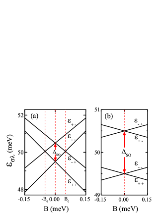
Figure 1: $\varepsilon_{\sigma\lambda}$ as a function of (a) parallel and (b) perpendicular magnetic fields for $\varepsilon_{d}=50\textrm{meV}$, $\mu=10$, and $\Delta_{SO}=1\textrm{meV}$.

Electronic transport through the CNT QD is determined by the dot retarded Green’s function, which is $G_{m}(\varepsilon)\equiv\langle\langle d_{m}|d_{m}^{\dagger}\rangle\rangle=G_{m}^{0}(\varepsilon)(1+U\sum_{m^{\prime}}\langle\langle\hat{n}_{m^{\prime}}d_{m}|d_{m}^{\dagger}\rangle\rangle)$, where $G_{m}^{0}\left(\varepsilon\right)=\left[\varepsilon-\varepsilon_{m}-\Sigma^{0}\left(\varepsilon\right)\right]^{-1}$, $\Sigma^{0}\left(\varepsilon\right)=\frac{\Gamma}{\pi}\int\frac{\textrm{d}\varepsilon^{\prime}}{\varepsilon-\varepsilon^{\prime}}$, $\Gamma=\sum_{\alpha}\Gamma_{\alpha}$, and $\Gamma_{\alpha}=\pi\rho|V_{\alpha}|^{2}$ with $\rho$ being the density of states in the leads at the Fermi level. Due to the interaction $U$, $G_{m}(\varepsilon)$ includes a high-order Green’s function, whose equation of motion (EOM) produces in turn more higher-order ones. We truncate this hierarchy by the Lacroix’s decoupling procedure Luo ; Entin-Wohlman ; Shiau which successfully captures the essential physics of the Kondo effect. By this scheme, in the limit of $U\to\infty$, the dot Green’s function is given by

$$G_{m}\left(\varepsilon\right)=\frac{1-\sum^{\prime}_{m^{\prime}}\langle\hat{n}_{m^{\prime}}\rangle-\sum^{\prime}_{m^{\prime}}A_{m^{\prime}m}}{[G_{m}^{0}(\varepsilon)]^{-1}+\sum^{\prime}_{m^{\prime}}[\Sigma^{0}\left(\varepsilon\right)A_{m^{\prime}m}-B_{m^{\prime}m}]},$$ (1)

where the prime in the summation means $m^{\prime}\neq m$ and

$$\langle\hat{n}_{m^{\prime}}\rangle=-\frac{1}{\pi}\int\textrm{d}\varepsilon f_{0}\left(\varepsilon\right)\operatorname{Im}\left[G_{m^{\prime}}\left(\varepsilon\right)\right],$$ (2)

$$A_{m^{\prime}m}=\frac{\Gamma}{\pi}\int\textrm{d}\varepsilon^{\prime}f_{0}\left(\varepsilon^{\prime}\right)\frac{\left[G_{m^{\prime}}\left(\varepsilon^{\prime}\right)\right]^{\ast}}{\varepsilon+\varepsilon_{m^{\prime}}-\varepsilon_{m}-\varepsilon^{\prime}},$$ (3)

$$B_{m^{\prime}m}=\frac{\Gamma}{\pi}\int\textrm{d}\varepsilon^{\prime}f_{0}\left(\varepsilon^{\prime}\right)\frac{1+\left[\Sigma^{0}\left(\varepsilon^{\prime}\right)G_{m^{\prime}}(\varepsilon^{\prime})\right]^{\ast}}{\varepsilon+\varepsilon_{m^{\prime}}-\varepsilon_{m}-\varepsilon^{\prime}},$$ (4)

with $f_{0}\left(\varepsilon\right)=\left(1/\Gamma\right)\sum_{\alpha}\Gamma_{\alpha}f_{\alpha}(\varepsilon)$ where $f_{\alpha}(\varepsilon)$ represents the Fermi distribution function in the leads. Eqs. (1)-(4) can be solved self-consistently. For a QD with an $N$-fold degenerate level, $\varepsilon_{m}=\varepsilon_{d}$, an $SU(N)$ Kondo temperature within EOM is $T^{(N)}_{K}=D\exp\{\pi\varepsilon_{d}/[(N-1)\Gamma]\}$ note , where $D$ is the half bandwidth in the leads and $\varepsilon_{d}$ is measured from the Fermi level.

Results and discussions.—Experimentally, the measured differential conductance $dI/dV$ near zero source-drain bias directly reflects the Kondo features in the dot density of states $\rho_{d}(\varepsilon)=-\left(1/\pi\right)\sum_{m}\textrm{Im}[G_{m}(\varepsilon)]$. Within the Keldysh formalism book2 , the transport current is $I=\frac{4e}{h}\frac{\Gamma_{L}\Gamma_{R}}{\Gamma}\int\textrm{d}\varepsilon\;[f_{L}(\varepsilon)-f_{R}(\varepsilon)]\sum_{m}\textrm{Im}[G_{m}(\varepsilon)]$. In the numerical results presented below, we use symmetric dot-lead couplings $\Gamma_{L}=\Gamma_{R}$ and a symmetrically applied source-drain bias $V$. The high-energy cutoff is fixed to be $D=1$ and $\Gamma=0.01D$.

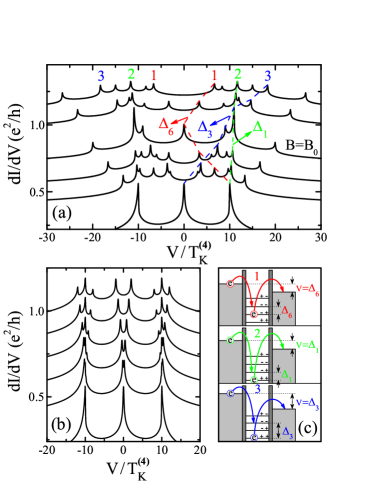
Figure 2: Fine structures of the Kondo resonance with spin-orbit coupling. (a) $dI/dV$ versus $V$ with various parallel magnetic fields, $B/B_{0}=0$ (bottom), $1/3$, $2/3$, $1$, $4/3$, $5/3$ (top). The red, green, and blue dashed lines are guides for the traces of peak pairs marked by the numbers $1$, $2$, and $3$, respectively. (b) $dI/dV$ versus $V$ with various perpendicular magnetic fields, $B/T^{(4)}_{K}=0$ (bottom), $0.1$, $0.2$, $0.4$, $0.7$, $1$ (top). (c) Schematic representation of three transition processes producing the peak pairs $1$, $2$, and $3$ in (a), respectively. In (a) and (b), the curves corresponding to $B\neq 0$ are offset for clarity. The parameters used are $\varepsilon_{d}=-10\Gamma$, $\mu=10$, and $\Delta_{SO}=10T^{(4)}_{K}$.

Figure 3: $SU(4)$ Kondo splitting without spin-orbit coupling. (a) $dI/dV$ versus $V$ with different parallel magnetic fields, $B/T^{(4)}_{K}=0$ (bottom), $0.05$, $0.1$, $0.2$, $0.4$, $0.6$ (top). (b) $dI/dV$ versus $V$ with different perpendicular magnetic fields, $B/T^{(4)}_{K}=0$ (bottom), $0.5$, $1$, $2$, $4$, $6$ (top). The curves corresponding to $B\neq 0$ are offset for clarity. The parameters used are $\varepsilon_{d}=-10\Gamma$, $\mu=10$, and $\Delta_{SO}=0$.

Figure 2 presents our main results. Even at zero magnetic field, the spin-orbit coupling lifts the degeneracy in parallel and anti-parallel spin-orbit configurations of a single electron in the dot [see Fig. 1], thereby breaking the $SU(4)$ symmetry of the Kondo effect studied previously Choi ; Lim ; Busser ; Anders . Instead, the Kondo effect manifests as three resonant peaks in the differential conductance, which locate at $V=0$, $\pm\Delta_{SO}$, respectively. Due to the coupling, each peak entangles both spin and orbital degrees of freedom. Specifically, the two side peaks arise from both spin-flip intraorbital and spin-conserved interorbital transitions, while the central peak is attributed to spin-flip interorbital transitions. A similar zero-field three-peak structure has also been predicted in Silicon QDs Shiau but the underlying mechanism is entirely different. In Shiau , the two side peaks result from a trivial valley (orbital) splitting at zero field and the remaining spin degeneracy gives rise to the central peak.

When the magnetic field is applied, the Zeeman effect further removes the remaining degeneracies in the energy spectrum and the situation becomes complicated. In the field along the tube axis [Fig. 2(a)], owing to the interplay of spin-orbit coupling and Zeeman effect, each peak at zero field further splits into four subpeaks, ending up with rich twelve-peak structures in the Kondo resonance. At $B=B_{0}$, only seven peaks are visible and the other peaks merge into the remaining ones. This is because of the level degeneracy at this special field [see Fig. 1(a)]. Though these fine multipeak structures appear to be complicated, the inherent physics and the $B$-evolution of each peak can be clarified by identifying all many-body cotunnelings that add up coherently to screen both spin and orbital degrees of freedom.

In the one-electron regime, the Kondo effect arises from the coherent superposition of six transition processes: two spin-flip intraorbital transitions $|\sigma,\lambda\rangle\Leftrightarrow|-\sigma,\lambda\rangle$, two spin-flip interorbital transitions $|\sigma,\lambda\rangle\Leftrightarrow|-\sigma,-\lambda\rangle$, and two spin-conserved interorbital transitions $|\sigma,\lambda\rangle\Leftrightarrow|\sigma,-\lambda\rangle$. Each transition needs an energy of $\Delta_{i}$ ($i=1,\cdots,6$) and develops a pair of Kondo peaks at $V=\pm\Delta_{i}$. From energy differences between the initial and final states, one readily lists all six transition energies as $\Delta_{1}=\left|\varepsilon_{++}-\varepsilon_{-+}\right|$, $\Delta_{2}=\left|\varepsilon_{+-}-\varepsilon_{--}\right|$, $\Delta_{3}=\left|\varepsilon_{++}-\varepsilon_{--}\right|$, $\Delta_{4}=\left|\varepsilon_{+-}-\varepsilon_{-+}\right|$, $\Delta_{5}=\left|\varepsilon_{++}-\varepsilon_{+-}\right|$, and $\Delta_{6}=\left|\varepsilon_{-+}-\varepsilon_{--}\right|$. Both the spin-orbit coupling and the magnetic field are symmetry-breaking perturbations at the $SU(4)$ Kondo fixed point. For $\Delta_{SO}=B=0$ and hence $\Delta_{i}=0$, the fixed point is reached Choi ; Lim . Thus all the cotunneling processes are elastic and constitute a highly symmetric $SU(4)$ Kondo resonance at $V=0$ (see the curve corresponding to $B=0$ in Fig. 3). On the other hand, one can uniquely identify the six transition processes from the split Kondo peaks as long as all $\Delta_{i}$ are different from each other and hence the six peak pairs (twelve peaks) are well resolved, which requires $\Delta_{SO}\neq 0$, $B\neq 0$, and $\cos\theta\neq 0$. This is exactly the case of Fig. 2(a). As an example, we trace the $B$-evolutions of three peak pairs marked by the numbers $1$, $2$, and $3$ and unambiguously attribute them to transition processes $|-,+\rangle\Leftrightarrow|-,-\rangle$, $|+,+\rangle\Leftrightarrow|-,+\rangle$, and $|+,+\rangle\Leftrightarrow|-,-\rangle$, respectively, which are schematically shown in Fig. 2(c). We also note that such an unique identification is unavailable in Silicon QDs Shiau where no more than nine peaks are visible.

When the field is applied perpendicularly to the CNT, the orbital Zeeman effect is absent and only the spin Zeeman effect is involved. As shown in Fig. 2(b), while the central peak splits into two subpeaks corresponding to the spin-flip interorbital transitions, the two side peaks split into three subpeaks among which the two split-off ones result from the spin-flip intraorbital transitions and the rested one corresponds to the interorbital transitions without spin-flip. In this case, some peaks are still not resolved because $\Delta_{3}=\Delta_{4}$ and $\Delta_{5}=\Delta_{6}$.

It is useful to comment on the experimental observability of these fine multipeak structures. On the one hand, in our EOM scheme the Kondo temperature is underestimated and relatively, the splitting of the Kondo peaks is more evident. On the other hand, the decoherence Meir1993 neglected in the present study has an effect to smear out the split peaks, especially those with high energies. These two features will make the observation a bit difficult. However, in ultra-clean CNT QDs and using highly resolved spectroscopy measurements, it is still possible to observe part or all of these fine structures.

For comparison, we plot in Fig. 3 the multiple splitting of the $SU(4)$ Kondo resonance by neglecting the spin-orbit coupling. On increasing the field, the $SU(4)$ Kondo peak at the zero bias splits in a simple way following the Zeeman effect, which produces characteristic structures in agreement with the results in the literature Jarillo-Herrero1 ; Choi ; Lim ; Makarovski1 but quite different from that discussed above.

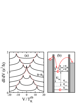
Figure 4: Purely orbital Kondo effect in the $2e$ regime. (a) $dI/dV$ versus $V$ with various parallel magnetic fields, $(B-B_{0})/T^{(2)}_{K}=-0.6$ (bottom), $-0.4$, $-0.2$, $0$, $0.2$, $0.4$, $0.6$ (top). The curves are offset for clarity and the parameters used are $\varepsilon^{\prime}_{d}=-3\Gamma$ and $\mu=10$. (b) Schematic diagram of the inherent many-body cotunneling.

The spin-orbit coupling further determines the filling order in the $2e$ ground state Kuemmeth , which exactly follows the first excited state of the single-particle spectrum (Fig. 1). At the parallel fields near the degenerate point $B_{0}$, while the first electron always occupies the state $|+,+\rangle$, the second electron can fluctuate between $|-,-\rangle$ and $|-,+\rangle$, giving rise to a purely orbital Kondo effect as its spin $\sigma=-$ is fixed. To describe this Kondo effect, $m$ appearing in all our previous formulae should be replaced by $\{-,\lambda\}$ and the single-particle energy becomes $\varepsilon^{\prime}_{-\lambda}\equiv\varepsilon_{-\lambda}+U_{2e}=\varepsilon^{\prime}_{d}+(1-\lambda\mu)(B-B_{0})$, where $U_{2e}$ is the $2e$ Coulomb interaction and $\varepsilon^{\prime}_{d}=\varepsilon_{d}+\Delta_{SO}/(2\mu)+U_{2e}$. Fig. 4(a) presents the resulting $dI/dV$ as a function of $V$. For $B=B_{0}$, there is a pronounced zero-bias peak which represents an $SU(2)$ orbital Kondo effect and provides a spin-polarized conducting channel. The peak splits due to the field applied away from the degenerate point. This orbital Kondo effect, as schematically shown in Fig. 4(b), comes from the same shell and dwells in the $2e$ valley, therefore being distinct from the one recently observed in CNT QDs without spin-orbit coupling Jarillo-Herrero1 .

Conclusion.—We have studied the Kondo effect in a CNT QD with spin-orbit coupling. It is shown that the Kondo effect manifests as rich fine multipeak structures in the differential conductance when a magnetic field is applied. These fine structures are quite different from the $SU(4)$ Kondo effect studied previously and might be observable in future experiments. In such a system, a purely orbital Kondo effect develops in the $2e$ ground state due to the particular multielectron filling order. Our results indicate that the spin-orbit coupling significantly changes the low-energy Kondo physics in CNT QDs.

Support from the NSFC (10575119), the Major State Basic Research Developing Program (2007CB815004), and the Program for NCET of China is acknowledged.

References

- (1) A. C. Hewson, The Kondo Problem to Heavy Fermions (Cambridge University Press, Cambridge, 1993).
- (2) D. Goldhaber-Gordon et al., Nature (London) 391, 156 (1998); S. M. Cronenwett, T. H. Oosterkamp, and L. P. Kouwenhoven, Science 281, 540 (1998).
- (3) T. K. Ng and P. A. Lee, Phys. Rev. Lett. 61, 1768 (1988); L. I. Glazman and M. E. Raikh, Pis’ma Zh. Eksp. Teor. Fiz. 47, 378 (1988) [JETP Lett. 47, 452 (1988)].
- (4) J. Nygård, D. H. Cobden, and P. E. Lindelof, Nature (London) 408, 342 (2000).
- (5) M. R. Buitelaar et al., Phys. Rev. Lett. 88, 156801 (2002); B. Babić, T. Kontos, and C. Schönenberger, Phys. Rev. B 70, 235419 (2004).
- (6) P. Jarillo-Herrero et al., Nature (London) 434, 484 (2005).
- (7) P. Jarillo-Herrero et al., Phys. Rev. Lett. 94, 156802 (2005).
- (8) A. Makarovski et al., Phys. Rev. B 75, 241407(R) (2007).
- (9) A. Makarovski, J. Liu, and G. Finkelstein, Phys. Rev. Lett. 99, 066801 (2007).
- (10) W. J. Liang, M. Bockrath, and H. Park, Phys. Rev. Lett. 88, 126801 (2002).
- (11) M.-S. Choi, R. López, and R. Aguado, Phys. Rev. Lett. 95, 067204 (2005).
- (12) J.-S. Lim et al., Phys. Rev. B 74, 205119 (2006).
- (13) C. A. Büsser and G. B. Martins, Phys. Rev. B 75, 045406 (2007).
- (14) F. B. Anders et al., Phys. Rev. Lett. 100, 086809 (2008).
- (15) D. Huertas-Hernando, F. Guinea, and A. Brataas, Phys. Rev. B 74, 155426 (2006); D. V. Bulaev, B. Trauzettel, and D. Loss, Phys. Rev. B 77, 235301 (2008).
- (16) F. Kuemmeth et al., Nature (London) 452, 448 (2008).
- (17) E. D. Minot et al., Nature (London) 428, 536 (2004).
- (18) C. Lacroix, J. Phys. F: Metal Phys. 11, 2389 (1981); H. G. Luo, Z. J. Ying, and S. J. Wang, Phys. Rev. B 59, 9710 (1999).
- (19) O. Entin-Wohlman, A. Aharony, and Y. Meir, Phys. Rev. B 71, 035333 (2005); V. Kashcheyevs, A. Aharony, and O. Entin-Wohlman, Phys. Rev. B 73, 125338 (2006).
- (20) S. Y. Shiau, S. Chutia, and R. Joynt, Phys. Rev. B 75, 195345 (2007); S. Y. Shiau, and R. Joynt, Phys. Rev. B 76, 205314 (2007).
- (21) This expression is slightly different from given by the renormalization group scaling theory Choi ; Lim . The difference is due to the present truncation approximation, which can be improved by involving more higher-order Green’s functions Luo .
- (22) H. Haug and A.-P. Jauho, Quantum Kinetics in Transport and Optics of Semiconductors (Springer, Berlin, 1998).
- (23) Y. Meir, N. S. Wingreen and P. A. Lee, Phys. Rev. Lett. 70, 2601 (1993).