Counting the Faces of Randomly-Projected Hypercubes and Orthants, with Applications

Abstract.

Let $A$ be an $n$ by $N$ real valued random matrix, and $H^{N}$ denote the $N$-dimensional hypercube. For numerous random matrix ensembles, the expected number of $k$-dimensional faces of the random $n$-dimensional zonotope $AH^{N}$ obeys the formula $Ef_{k}(AH^{N})/f_{k}(H^{N})=1-P_{N-n,N-k}$, where $P_{N-n,N-k}$ is a fair-coin-tossing probability:

$$P_{N-n,N-k}\equiv\mbox{Prob}\{N-k-1\mbox{ or fewer successes in }N-n-1\mbox{ tosses }\}.$$

The formula applies, for example, where the columns of $A$ are drawn i.i.d. from an absolutely continuous symmetric distribution. The formula exploits Wendel’s Theorem[19].

Let ${\mathbb{R}}_{+}^{N}$ denote the positive orthant; the expected number of $k$-faces of the random cone$A{\mathbb{R}}_{+}^{N}$ obeys ${\mathcal{E}}f_{k}(A{\mathbb{R}}_{+}^{N})/f_{k}({\mathbb{R}}_{+}^{N})=1-P_{N-n,N-k}$. The formula applies to numerous matrix ensembles, including those with iid random columns from an absolutely continuous, centrally symmetric distribution.

The probabilities $P_{N-n,N-k}$ change rapidly from nearly 0 to nearly 1 near $k\approx 2n-N$. Consequently, there is an asymptotically sharp threshold in the behavior of face counts of the projected hypercube; thresholds known for projecting the simplex and the cross-polytope, occur at very different locations. We briefly consider face counts of the projected orthant when $A$ does not have mean zero; these do behave similarly to those for the projected simplex. We consider non-random projectors of the orthant; the ’best possible’ $A$ is the one associated with the first $n$ rows of the Fourier matrix.

These geometric face-counting results have implications for signal processing, information theory, inverse problems, and optimization. Most of these flow in some way from the fact that face counting is related to conditions for uniqueness of solutions of underdetermined systems of linear equations.

a) A vector in ${\mathbb{R}}_{+}^{N}$ is called $k$-sparse if it has at most $k$ nonzeros. For such a $k$-sparse vector $x_{0}$, let $b=Ax_{0}$, where $A$ is a random matrix ensemble covered by our results. With probability $1-P_{N-n,N-k}$ the inequality-constrained system $Ax=b$, $x\geq 0$ has $x_{0}$ as its unique nonnegative solution. This is so, even if $n<N$, so that the system $Ax=b$ is underdetermined.

b) A vector in the hypercube $H^{N}$ will be called $k$-simple if all entries except at most $k$ are at the bounds 0 or 1. For such a $k$-simple vector $x_{0}$, let $b=Ax_{0}$, where $A$ is a random matrix ensemble covered by our results. With probability $1-P_{N-n,N-k}$ the inequality-constrained system $Ax=b$, $x\in H^{N}$ has $x_{0}$ as its unique solution in the hypercube.

Keywords. Zonotope, Random Polytopes, Random Cones, Wendel’s Theorem, Threshold Phenomena, Universality, Random Matrices, Compressed Sensing, Unique Solution of Underdetermined Systems of Linear Equations.

1. Introduction

There are 3 fundamental regular polytopes in ${\mathbb{R}}^{N}$, $N\geq 5$: the hypercube $H^{N}$, the cross-polytope $C^{N}$, and the simplex $T^{N-1}$. For each of these, projecting the vertices into ${\mathbb{R}}^{n}$, $n<N$, yields the vertices of a new polytope; in fact, every polytope in $R^{n}$ can be generated by rotating the simplex $T^{N-1}$ and orthogonally projecting on the first $n$ coordinates, for some choice of $N$ and of $N$-dimensional rotation. Similarly, every centro-symmetric polytope can be generated by projecting the cross-polytope, and every zonotope by projecting the hypercube.

1.1. Random polytopes

Choosing the projection $A$ at random has become popular. Let $A$ be an $n\times N$ uniformly distributed random orthogonal projection, obtained by first applying a uniformly-distributed rotation to ${\mathbb{R}}^{N}$ and then projecting on the first $n$ coordinates. Let $Q$ be a polytope in ${\mathbb{R}}^{N}$. Then $AQ$ is a random polytope in ${\mathbb{R}}^{n}$. Taking $Q$ in turn from each of the three families of regular polytopes we get three arenas for scholarly study:

• Random polytopes of the form $AT^{N-1}$ were first studied by Affentranger and Schneider [1] and by Vershik and Sporyshev [18];

• Random polytopes of the form $AC^{N}$ were first studied extensively by Borozcky and Henk [5];

• The random zonotope $AH^{N}$ will be heavily studied in this paper; beginnings of a literature on zonotopes can be found in [4, 2].

Such random polytopes can have face lattices undergoing abrupt changes in properties as dimensions change only slightly. In the case of $AT^{N-1}$ and $AC^{N}$, previous work by the authors [7, 10, 13, 12] documented the following t͡hreshold phenomenon. (Our work built on fundamental formulas developed by Affentranger and Schneider [1] and used an asymptotic framework pioneered by Vershik and Sporyshev [18], who pointed to the first such threshold effect). Let $f_{k}(Q)$ denote the number of $k$-dimensional faces of polyhedron $Q$. It turns out that for large $n$, the number of $k$-dimensional faces of $f_{k}(AQ)$ might either be approximately equal to $f_{k}(Q)$ or else significantly smaller, depending on the size of $k$ relative to a threshold depending on the ratio of $n$ to $N$.

To make this precise, consider the following proportional-dimensional asymptotic framework. A dimension specifier is a triple of integers $(k,n,N)$, representing a ‘face’ dimension $k$, a ‘small’ dimension $n$ and a ‘large’ dimension $N$; $k<n<N$. For fixed $\delta,\rho\in(0,1)$, consider sequences of dimension specifiers, indexed by $n$, and obeying

(1.1) $$k_{n}/n\rightarrow\rho\quad\mbox{ and }\quad n/N_{n}\rightarrow\delta.$$

For such sequences the small dimension $n$ is held proportional to the large dimension $N$ as both dimensions grow. We omit subscripts on $k_{n}$ and $N_{n}$ when possible. For $Q=T^{N-1}$, $C^{N}$, the papers [7, 10, 13, 12] exhibited thresholds $\rho(\delta;Q)$ for for the ratio between the expected number of faces of the low-dimensional polytope $AQ$ and the number of faces of the high-dimensional polytope $Q$:

(1.2) $$\lim_{n\rightarrow\infty}\frac{{\mathcal{E}}f_{k}(AQ)}{f_{k}(Q)}\quad\left\{\begin{array}[]{cl}=1&\rho<\rho_{W}(\delta;Q)\\ <1&\rho>\rho_{W}(\delta;Q)\end{array}\right..$$

(In this relation, we take a limit as $n\rightarrow\infty$ along some sequence obeying the proportional-dimensional constraint (1.1)). In words, the random object $AQ$ has roughly as many $k$-faces as its generator $Q$, for $k$ below a threshold; and has noticeably fewer $k$-faces than $Q$, for $k$ above the threshold. The threshold functions are defined in terms of Gaussian integrals and other special functions, and can be calculated numerically.

These phenomena, described here from the viewpoint of combinatorial geometry, have surprising consequences in probability theory, information theory and signal processing; see [8, 11, 13], and Section 5 below.

1.2. Random Zonotopes

Missing from the above picture is information about the third family of regular polytopes, the hypercube. Böröczky and Henk [5] discussed it in passing, but only considered the asymptotic framework where the small dimension $n$ is held fixed while the large dimension $N\rightarrow\infty$. In that framework, the threshold phenomenon is not visible. In this paper, we again consider the proportional-dimensional case (1.1) and prove the following.

Theorem 1.1 (‘Weak’ Threshold for Hypercube).

Let

(1.3) $$\rho_{W}(\delta;H^{N}):=\max{(0,2-\delta^{-1})}.$$

For $\rho$,$\delta$ in $(0,1)$, consider a sequence of dimension specifiers $(k,n,N)$ obeying (1.1). Let $A$ denote a uniformly-distributed random orthogonal projection from ${\mathbb{R}}^{N}$ to ${\mathbb{R}}^{n}$.

(1.4) $$\lim_{n\rightarrow\infty}\frac{{\mathcal{E}}f_{k}(AH^{N})}{f_{k}(H^{N})}=\left\{\begin{array}[]{cl}1,&\rho<\rho_{W}(\delta,H^{N})\\ 0,&\rho>\rho_{W}(\delta,H^{N})\end{array}\right..$$

Thus we prove a sharp discontinuity in the behavior of the face lattices of random zonotopes; the location of the threshold is precisely identified. (Such sharpness of the phase transition is also observed empirically for (1.2) above; to our knowledge, a proof of discontinuity has not yet been published in that setting. ) Our use of the modifier ‘weak’ and the subscript $W$ on $\rho$ matches usage in the previous cases $T^{N-1}$ and $C^{N}$.

Although this result has been stated in the language of combinatorial convexity, as with the earlier results for $AT^{N-1}$ and $AC^{N}$, there are implications for applied fields including optimization and signal processing, see Section 5 below.

1.3. More General Notion of Random Projection

In fact, Theorem 1.1 is only the tip of the iceberg. The ensemble of random matrices used in that result - uniformly distributed random orthoprojector - is only one example of a random matrix ensemble for which the conclusion (1.4) holds. As it turns out, what really matters are the statistical properties of the nullspace of $A$.

Definition 1.2 (Orthant-Symmetry).

Let $B$ be a random $N-n$ by $N$ matrix such that for each diagonal matrix $S$ with diagonal in $\{-1,1\}^{N}$, and for every measurable set $\Omega$,

$$\mbox{Prob}\{BS\in\Omega\}=\mbox{Prob}\{B\in\Omega\}.$$

Then we say that $B$ is an orthant-symmetric random matrix. Let $V_{B}$ be the linear span of the rows of $B$. If $B$ is an orthant-symmetric random matrix we say that $V$ is an orthant-symmetric random subspace.

Remark 1.3 (Orthant-Symmetric Ensembles).

The following ensembles of random matrices are orthant-symmetric:

• Uniformly-distributed Random orthoprojectors from ${\mathbb{R}}^{N}$ to ${\mathbb{R}}^{N-n}$; implicitly this was the example considered earlier.

• Gaussian Ensembles. A random matrix $B$ with entries chosen from a Gaussian zero-mean distribution, i.e. such that the $(N-n)\cdot N$-element vector $vec(B)$ is $N(0,\Sigma)$ with $\Sigma$ a nondegenerate covariance matrix.

• Symmetric i.i.d. Ensembles. Matrices with entries sampled i.i.d. from a symmetric probability distribution; examples include Gaussian $N(0,1)$, uniform on $[-1,1]$, uniform from the set $\{-1,1\}$, and from the set $\{-1,0,1\}$ where $-1$ and $1$ have equal non-zero probability.

• Sign Ensembles. For any fixed generator matrix $B_{0}$, let the random matrix $B=B_{0}S$ where $S$ is a random diagonal matrix with entries drawn uniformly from $\{-1,1\}$.

New orthant-symmetric ensembles can be created from an existing one by multiplying on the left by an arbitrary random matrix $T$ which is stochastically independent of $B$, and multiplying on the right by a random diagonal matrix $R$ also stochastically independent of $B$ and $T$: thus $B^{\prime}=TBR$ inherits orthant symmetry from $B$.

Definition 1.4 (General Position).

Let $B$ be a random $N-n$ by $N$ matrix such that every subset of $N-n$ columns is almost surely linearly independent. Let $V_{B}$ be the linear span of the rows of $B$. We say that $V_{B}$ is a generic random subspace.

Many orthant-symmetric ensembles from our list create generic row spaces:

• Uniformly-distributed random orthoprojectors;

• Gaussian Ensembles;

• Symmetric iid ensembles having an absolutely continuous distribution;

• Sign Ensembles with generator matrix $B_{0}$ having its columns in general position;

Define a censored symmetric iid ensemble as a symmetric iid ensemble from which we discard realizations $B$ where the columns happen to be not in general position. Censoring a symmetric iid ensemble made from the Bernoulli $\{-1,+1\}$ coin tossing distribution produces a new random matrix model $\tilde{B}$ whose realizations are in general position with probability one. (The probability of a censoring event is exponentially small in $N$, [17]).

Theorem 1.5 (‘Weak’ Threshold for Hypercube ).

Let the random matrix $A$ have a random nullspace which is orthant symmetric and generic. In the proportional-dimensional framework (1.1) the random zonotope $AH^{N}$ obeys the same conclusion (1.4) as in Theorem 1.1.

In a sense, this theorem extends the conclusion of Theorem 1.1 to vastly more cases . It has been previously observed that some results known for the Goodman-Pollack random orthoprojector model actually extend to other ensembles of random matrices. It was observed for the simplex by Affentranger and Schneider [1], and proven by Baryshnikov and Vitale [3, 2], that face-counting results known for uniformly-distributed random orthoprojectors follow as well for Gaussian iid matrices $A$.

Our extension of Theorem 1.1 from orthoprojectors to orthant-symmetric null spaces in Theorem 1.5 follows this program. However, it is a vastly larger extension.

1.4. Random Cone

Convex cones provide another type of fundamental polyhedral set. Amongst these, the simplest and most natural is the positive orthant $P={\mathbb{R}}_{+}^{N}$. The image of a cone under projection $A$: ${\mathbb{R}}^{N}\rightarrow{\mathbb{R}}^{n}$ is again a cone $K=AP$. Typically the cone has $f_{0}(K)=1$ vertex (at 0), and $f_{1}(K)=N$ extreme rays, etc. In fact, every such pointed cone in ${\mathbb{R}}^{n}$ can be generated as a projection of the positive orthant, with an appropriate orthogonal projection from an appropriate ${\mathbb{R}}^{N}$.

As with the polytopes models, surprising threshold phenomena can arise when the projector is random.

Theorem 1.6 (‘Weak’ Threshold for Orthant).

Let $A$ be a random matrix whose nullspace is an orthant-symmetric and generic random subspace. In the proportional-dimensional framework (1.1) we have

(1.5) $$\lim_{n\rightarrow\infty}\frac{{\mathcal{E}}f_{k}(A{\mathbb{R}}_{+}^{N})}{f_{k}({\mathbb{R}}_{+}^{N})}=\left\{\begin{array}[]{cl}1,&\rho<\rho_{W}(\delta;{\mathbb{R}}_{+}^{N})\\ 0,&\rho>\rho_{W}(\delta;{\mathbb{R}}_{+}^{N})\end{array}\right.$$

with $\rho_{W}(\delta;{\mathbb{R}}_{+}^{N})\equiv\rho_{W}(\delta;H^{N})$ as defined in (1.3).

Here the threshold for the orthant is at precisely the same place as it was for the hypercube. Theorem 1.6 is proven in Section 2.3, and there are significant implications in optimization and signal processing briefly discussed in Section 5.

1.5. Exact equality in the number of faces

Our focus in Sections 1.1-1.4 has been on the ‘weak’ agreement of ${\mathcal{E}}f_{k}(AQ)$ with $f_{k}(Q)$; we have seen in the proportional-dimensional framework, for $\rho$ below threshold $\rho_{W}(\delta;Q)$, we have limiting relative equality:

$$\frac{{\mathcal{E}}f_{k}(A{\mathbb{R}}_{+}^{N})}{f_{k}({\mathbb{R}}_{+}^{N})}\rightarrow 1,\qquad n\rightarrow\infty.$$

We now focus on the ‘strong’ agreement; it turns out that in the proportional dimensional framework, for $\rho$ below a somewhat lower threshold $\rho_{S}(\delta;Q)$, we actually have exact equality with overwhelming probability:

(1.6) $$\mbox{Prob}\{f_{k}(Q)=f_{k}(AQ)\}\rightarrow 1,\qquad n\rightarrow\infty.$$

The existence of such ‘strong’ thresholds for $Q=T^{N-1}$ and $Q=C^{N}$ was proven in [7, 10], which exhibited thresholds $\rho_{S}(\delta;Q)$ below which (1.6) occurs. These “strong thresholds” and the previously mentioned “weak thresholds” (1.2) are depicted in Figure 3.1. A similar strong threshold also holds for the projected orthant.

Theorem 1.7 (‘Strong’ Threshold for Orthant).

Let

(1.7) $$H(\gamma):=\gamma\log(1/\gamma)-(1-\gamma)\log(1-\gamma)$$

denote the usual (base-$e$) Shannon Entropy. Let

(1.8) $$\psi_{S}^{{\mathbb{R}}_{+}}(\delta,\rho):=H(\delta)+\delta H(\rho)-(1-\rho\delta)\log 2.$$

For $\delta\geq 1/2$, let $\rho_{S}(\delta;{\mathbb{R}}_{+}^{N})$ denote the zero crossing of $\psi_{S}^{{\mathbb{R}}_{+}}(\delta,\rho)$. In the proportional-dimensional framework (1.1) with $\rho<\rho_{S}(\delta;{\mathbb{R}}_{+}^{N})$

(1.9) $$\mbox{Prob}\{f_{k}(A{\mathbb{R}}_{+}^{N})=f_{k}({\mathbb{R}}_{+}^{N})\}\rightarrow 1,\quad\quad\mbox{as}\;\;n\rightarrow\infty.$$

The threshold $\rho_{W}(\delta;Q)$ for $Q={\mathbb{R}}_{+}^{N}$ and $H^{N}$, and $\rho_{S}(\delta;{\mathbb{R}}_{+}^{N})$ are depicted in Figure 1.1.

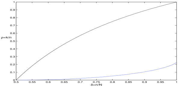
Figure 1.1. The ‘weak’ thresholds, $\rho_{W}(\delta;H^{N})$ and $\rho_{W}(\delta;{\mathbb{R}}_{+}^{N})$ (black), and a lower bound on the strong threshold for the positive orthant, $\rho_{S}(\delta;{\mathbb{R}}_{+}^{N})$ (blue).

In contrast to the projected simplex, cross-polytope, and orthant, for the hypercube, there is no nontrivial regime where a phenomenon like (1.6) can occur.

Lemma 1.8 (Zonotope Vertices).

Let $A$ be an $n\times N$ matrix, and let $H^{N}$ be the $N$ dimensional hypercube.

$$f_{k}(AH^{N})<f_{k}(H^{N}),\qquad k=0,1,2,\ldots n.$$

Proof of Theorem 1.8.

In fact, we will show that $AH^{N}$ always has fewer than $2^{N}$ vertices. This immediately implies the full result. There exists a $w\in{\mathcal{N}}(A)$ with $w\neq 0$. $H^{N}$ has a vertex $x_{0}$ obeying

$$x_{0}(i):=\left\{\begin{array}[]{ll}0&\mbox{sgn}(w(i))>0,\\ 1&\mbox{else}.\end{array}\right.$$

Let $x_{t}:=x+tw$ with $t>0$. For $t$ sufficiently small $x_{t}$ is in the interior of $H^{N}$, and by construction $Ax_{0}=Ax_{t}$. Invoking Lemma 2.5, $x_{0}$ is not a vertex of $AH^{N}$, and $f_{0}(AH^{N})<f_{0}(H^{N})$. ∎

Although this proof only highlights a single vertex of $H^{N}$ that is interior to $AH^{N}$, it is clear from its construction that there are typically many such lost vertices. Theorem 1.7 is proven in Section 2.5.

1.6. Exact Non-Asymptotic Results

We have so far exclusively used the Vershik-Sporyshev proportional-dimensional asymptotic framework; this makes for the most natural comparisons between results for the three families of regular polytopes. However, for the positive orthant and hypercube, something truly remarkable happens: there is a simple exact expression for finite $N$ which connects to a beautiful result in geometric probability.

Theorem 1.9 (Wendel, [19]).

Let $M$ points in ${\mathbb{R}}^{m}$ be drawn i.i.d. from a centro-symmetric distribution such that the points are in general position, then the probability that all the points fall in some half space is

(1.10) $$P_{m,M}=2^{-M+1}\sum_{\ell=0}^{m-1}{M-1\choose\ell}.$$

This elegant result is often presented as simply a piece of recreational mathematics. In our setting, it turns out to be truly powerful, because of the following identity.

Theorem 1.10.

Let $A$ be an $n\times N$ random matrix with an orthant-symmetric and generic random nullspace.

(1.11) $$\frac{{\mathcal{E}}f_{k}(A{\mathbb{R}}_{+}^{N})}{f_{k}({\mathbb{R}}_{+}^{N})}=1-P_{N-k,N-n}.$$

Symmetry implies a similar identity for the hypercube:

Theorem 1.11.

Let $A$ be a random matrix with an orthant-symmetric and generic random nullspace.

(1.12) $$\frac{{\mathcal{E}}f_{k}(AH^{N})}{f_{k}(H^{N})}=1-P_{N-n,N-k}.$$

These formulae are not at all asymptotic or approximate. But all the earlier asymptotic results derive from them. Theorem 1.10 is proven in Section 2.1, and the symmetry argument for Theorem 1.11 is formalized in Lemma 2.6 and proven in Section 6.3.

1.7. Contents

Theorem 1.6 is proven in Section 2.3, Theorems 1.1 and 1.5 are proven in Section 2.4, and Theorem 1.7 is proven in Section 2.5; each using the classical Wendel’s Theorem [19], Theorem 1.9. Their relationships with existing results in convex geometry and matroid theory are discussed in Section 3, the the implications of these results for information theory, signal processing, and optimization are briefly discussed in Section 5.

2. Proof of main results

Our plan is to start with the key non-asymptotic exact identity (1.11) and then derive from it Theorem 1.6 by asymptotic analysis of the probabilities in Wendel’s Theorem. We then infer Theorem 1.5 and later Theorem 1.7 follows in Section 2.5.

2.1. Proof of Theorem 1.10

Here and below we follow the convention that, if we don’t give the proof of a lemma or corollary immediately following its statement, then the proof can be found in Section 6.

Our proof of the key formula (1.11) starts with the following observation on the expected number of $k$-faces of ${\mathbb{R}}_{+}^{N}$.

(2.1) $$\frac{{\mathcal{E}}f_{k}(A{\mathbb{R}}_{+}^{N})}{f_{k}({\mathbb{R}}_{+}^{N})}=\mbox{Ave}_{F}\left[\mbox{Prob}\{AF\mbox{ is a $k$-face of }A{\mathbb{R}}_{+}^{N}\}\right].$$

Here $Ave_{F}$ denotes ”the arithmetic mean over all $k$-faces of ${\mathbb{R}}_{+}^{N}$.

Because of (2.1) we will be implicitly averaging across faces below. As a calculation device we suppose that all faces are statistically equivalent; this allows us to study one $k$-face, and yet compute the average across all $k$-faces.

Definition 2.1 (Exchangable columns).

Let $A$ be a random $n$ by $N$ matrix such that for each permutation matrix $\Pi$, and for every measurable set $\Omega$,

$$\mbox{Prob}\{A\in\Omega\}=\mbox{Prob}\{A\Pi\in\Omega\}$$

Then we say that $A$ has exchangeable columns.

Below we assume without loss of generality that $A$ has exchangeable columns. Then (2.1) becomes: let $F$ be a fixed $k$-face of ${\mathbb{R}}_{+}^{N}$; then

(2.2) $$\frac{{\mathcal{E}}f_{k}(A{\mathbb{R}}_{+}^{N})}{f_{k}({\mathbb{R}}_{+}^{N})}=\mbox{Prob}\{AF\mbox{ is a $k$-face of }A{\mathbb{R}}_{+}^{N}\}.$$

Let $P$ be a polytope in ${\mathbb{R}}^{N}$ and $x_{0}\in P$. The vector $v$ is a feasible direction for $P$ at $x_{0}$ if $x_{0}+tv\in P$ for all sufficiently small $t>0$. Let $\mbox{Feas}_{x_{0}}(P)$ denote the set of all feasible directions for $P$ at $x_{0}$.

Lemma 2.2.

Let $x_{0}$ be a vector in ${\mathbb{R}}_{+}^{N}$ with exactly $k$ nonzeros. Let $F$ denote the associated $k$-face of ${\mathbb{R}}_{+}^{N}$. For an $n\times N$ matrix $A$, let $AF$ denote the image of $F$ under $A$. The following are equivalent:

(Survive($A,F,{\mathbb{R}}_{+}^{N}$)):	$AF$ is a $k$-face of $A{\mathbb{R}}_{+}^{N}$,
(Transverse($A,x_{0},{\mathbb{R}}_{+}^{N}$))	${\mathcal{N}}(A)\cap\mbox{Feas}_{x_{0}}({\mathbb{R}}_{+}^{N})=\{0\}$.

We now develop the connections to the probabilities in Wendel’s theorem.

Lemma 2.3.

Let $x_{0}\in{\mathbb{R}}_{+}^{N}$ have $k$ nonzeros. Let $A$ be $n\times N$ with $n<N$ have an orthant-symmetric null space with exchangeable columns. Then

$$\mbox{Prob}\{(\mbox{Transverse($A,x_{0},{\mathbb{R}}_{+}^{N}$)})\;\;\mbox{Holds}\}=1-P_{N-n,N-k}$$

Proof.

Exchangeability of the columns implies that

$$\mbox{Prob}\{(\mbox{Transverse($A,x_{0},{\mathbb{R}}_{+}^{N}$)})\;\;\mbox{Holds}\}$$

does not depend on $x_{0}$ , but only on the number of nonzeros in $x_{0}$ and the size of $A$. Therefore, let $k$ be the number of nonzeros in $x_{0}$, and set

$$\pi_{k,n,N}\equiv\mbox{Prob}\{(\mbox{Transverse($A,x_{0},{\mathbb{R}}_{+}^{N}$)})\;\;\mbox{Holds}\}.$$

The matrix $A$ has its columns in general position. Therefore we may construct a basis $b_{i}$ for its null space, ${\mathcal{N}}(A)$, having exactly $N-n$ basis vectors. The $N$ by $N-n$ matrix $B^{T}$ having the $b_{i}$ for its columns generates every vector $w$ in ${\mathcal{N}}(A)$ via a product of the form $w=B^{T}c$, where $c\in{\mathbb{R}}^{N-n}$.

Without loss of generality, suppose the nonzeros of $x_{0}$ are in positions $i=N-k+1,\ldots,N$. Then $\mbox{Feas}_{x_{0}}({\mathbb{R}}_{+}^{N})=\{v\;:\;v_{1},\ldots v_{N-k}\geq 0\}$. Condition (Transverse($A,x_{0},{\mathbb{R}}_{+}^{N}$)) can be restated as

(2.3) $$\mbox{(Ineq)}\quad\left\{\begin{array}[]{l}\mbox{The only vector }c\mbox{ satisfying}\\ (B^{T}c)_{i}\geq 0,\quad i=1,\ldots,N-k,\\ \mbox{is the vector }c=0.\end{array}\right.$$

Suppose the contrary to (Ineq), i.e. suppose there is a $c\neq 0$ solving (2.3). Let now $\beta_{i}$ denote the $i$-th row of $B^{T}$, with $i=1,\ldots,N-k$. Then (2.3) is the same as

$$\beta_{i}\cdot c\geq 0,\quad i=1,\ldots,N-k.$$

Geometrically, this says that

Each vector $\beta_{i}$, $i=1,\ldots,N-k$,

falls in the half-space $\beta\cdot c\geq 0$.

Here $c$ is some fixed but arbitrary nonzero vector. Thus the event {(Ineq) does not hold} is equivalent to the event

All the vectors $\beta_{i}$ with $i=1,\ldots,N-k$

fall in some half-space of ${\mathbb{R}}^{N-n}$.

By our hypothesis, the vectors $\beta_{i}$ with $i=1,\ldots,N-k$ are drawn i.i.d. from a centrosymmetric distribution and are in general position. We now invoke Wendel’s Theorem, and it follows that

$$\pi_{k,n,N}=1-P_{N-n,N-k}.$$

∎

2.2. Some Generalities about Binomial Probabilities

The probability $P_{m,M}$ in Wendel’s theorem has a classical interpretation: it gives the probability of at most $m-1$ heads in $M-1$ tosses of a fair coin. The usual Normal approximation to the binomial tells us that

$$P_{m,M}\approx\Phi\left(\frac{(m-1)-(M-1)/2}{\sqrt{(M-1)/4}}\right),$$

with $\Phi$ the usual standard normal distribution function $\Phi(x)=\int_{-\infty}^{x}e^{-y^{2}/2}dy/\sqrt{2\pi}$; here the approximation symbol $\approx$ can be made precise using standard limit theorems, eg. appropriate for small or large deviations. In this expression, the approximating normal has mean $(M-1)/2$ and standard deviation $\sqrt{(M-1)/4}$. There are three regimes of interest, for large $m$, $M$, and three behaviors for $P_{m,M}$.

• Lower Tail: $m\ll M/2-\sqrt{M/4}$. $P_{m,M}\approx 0$.

• Middle: $m\approx M/2$. $P_{m,M}\in(0,1)$.

• Upper Tail: $m\gg M/2+\sqrt{M/4}$. $P_{m,M}\approx 1$.

2.3. Proof of Theorem 1.6

Using the correspondence $N-n\leftrightarrow m$, $N-k\leftrightarrow M$, and the connection to Wendel’s theorem, we have three regimes of interest:

• $N-n\ll(N-k)/2$

• $N-n\approx(N-k)/2$

• $N-n\gg(N-k)/2$

In the proportional-dimensional framework, the above discussion translates into three separate regimes, and separate behaviors we expect to be true:

• Case 1: $\rho<\rho_{W}(\delta;H^{N})$. $P_{N_{n}-n,N_{n}-k_{n}}\rightarrow 0$.

• Case 2: $\rho=\rho_{W}(\delta;H^{N})$. $P_{N_{n}-n,N_{n}-k_{n}}\in(0,1)$.

• Case 3 $\rho>\rho_{W}(\delta;H^{N})$. $P_{N_{n}-n,N_{n}-k_{n}}\rightarrow 1$.

Case $2$ is trivially true, but it has no role in the statement of Theorem 1.6. Cases 1 and 3 correspond exactly to the two parts of (1.5) that we must prove.

To prove Cases 1 and 3, we need an upper bound deriving from standard large-deviations analysis of the lower tail of the binomial.

Lemma 2.4.

Let $N-n<(N-k)/2$.

(2.4) $$P_{N-n,N-k}\leq n^{3/2}\exp\left(N\psi_{W}^{{\mathbb{R}}_{+}}\left(\frac{n}{N},\frac{k}{n}\right)\right)$$

where the exponent is defined as

(2.5) $$\psi_{W}^{{\mathbb{R}}_{+}}(\delta,\rho):=H(\delta)+\delta H(\rho)-H(\rho\delta)-(1-\rho\delta)\log 2$$

with $H(\cdot)$ the Shannon Entropy (1.7)

Proof. Upperbounding the sum in $P_{N-n,N-k}$ by $N-n-1$ times ${N-k-1\choose N-n}$ we arrive at

(2.6) $$P_{N-n,N-k}\leq 2^{N-k-1}\frac{n-k}{N-k}\cdot(N-k+1){N\choose n}{n\choose k}{N\choose k}^{-1}.$$

We can bound ${m\choose\gamma\cdot m}$ for $\gamma<1$ using the Shannon entropy (1.7):

(2.7) $$c_{1}n^{-1/2}e^{mH(\gamma)}\leq{m\choose\gamma\cdot m}\leq c_{2}e^{mH(\gamma)}$$

where $c_{1}:=\frac{16}{25}\sqrt{2/\pi}$, $c_{2}:=5/4\sqrt{2\pi}$. Recalling the definition of $\psi_{W}^{{\mathbb{R}}_{+}}$, we obtain (2.4). ∎

We will now consider Cases 1 and 3, and prove the corresponding conclusion.

Case 1: $\rho<\rho_{W}(\delta;{\mathbb{R}}_{+}^{N})$. The threshold function $\rho_{W}(\delta;{\mathbb{R}}_{+}^{N})$ is defined as the zero level curve $\psi_{W}^{H}(\delta,\rho_{W}(\delta;{\mathbb{R}}_{+}^{N}))=0$; thus for any $\rho$ strictly below $\rho_{W}(\delta;{\mathbb{R}}_{+}^{N})$, the exponent $\psi_{W}^{{\mathbb{R}}_{+}}(\delta,\rho)$ is strictly negative. Lemma 2.4 thus implies that $P_{N_{n}-n,N_{n}-k_{n}}\rightarrow 0$ as $n\rightarrow\infty$.

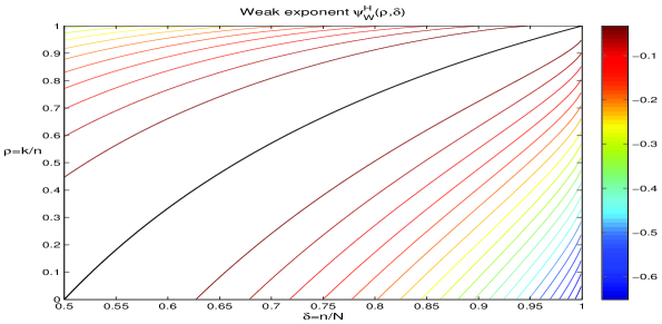
Figure 2.1. Exponent for the weak phase transition, $\psi_{W}^{{\mathbb{R}}_{+}}(\rho,\delta)$, (2.5), which has its zero level curve at $\rho_{W}(\delta;{\mathbb{R}}_{+}^{N})$, equation (1.3). The projected hypercube has the same weak phase transition and exponent $\psi_{W}^{H}\equiv\psi_{W}^{{\mathbb{R}}_{+}}$.

Case 3: $\rho>\rho_{W}(\delta;{\mathbb{R}}_{+}^{N})$. Binomial probabilities have a standard symmetry (relabel every ‘head’ outcome as a ’tail’, and vice versa). It follows that $P_{m,M}=1-P_{M-m,M}$. We have $P_{N-k,N-n}=1-P_{N-k,n-k}$. In this case $N-n>(N-k)/2$, so Lemma 2.4 tells us that $P_{N-k,n-k}\rightarrow 0$ as $n\rightarrow\infty$; we conclude $P_{N-k,N-n}\rightarrow 1$ as $n\rightarrow\infty$.

2.4. Proofs of Theorems 1.1 and 1.5

We derive the exact non-asymptotic result Theorem 1.11 from Theorem 1.10 by symmetry. The limit results in Theorems 1.1 and 1.5 follow immediately from asymptotic analysis of Section 2.3.

We begin as before, relating face counts to probabilities of survival.

(2.8) $$\frac{{\mathcal{E}}f_{k}(AH^{N})}{f_{k}(H^{N})}=\mbox{Ave}_{F}\left[\mbox{Prob}\{AF\mbox{ is a $k$-face of }AH^{N}\}\right].$$

Here $\mbox{Ave}_{F}$ denotes the average over $k$-faces of $H^{N}$.

As before, we assume exchangeable columns as a calculation device, allowing us to focus on one $k$-face, but compute the average. Under exchangeability, for any fixed $k$-face $F$,

(2.9) $$\frac{{\mathcal{E}}f_{k}(AH^{N})}{f_{k}(H^{N})}=\mbox{Prob}\{AF\mbox{ is a $k$-face of }AH^{N}\}.$$

We also again reformulate matters in terms of transversal intersection.

Lemma 2.5.

Let $x_{0}$ be a vector in $H^{N}$ with exactly $k$ nonzeros. Let $F$ denote the associated $k$-face of $H^{N}$. For an $n\times N$ matrix $A$ the following are equivalent: (Survive($A,F,H^{N}$)): $AF$ is a $k$-face of $AH^{N}$, (Transverse($A,x_{0},H^{N}$)): ${\mathcal{N}}(A)\cap\mbox{Feas}_{x_{0}}(H^{N})=\{0\}$.

We next connect the hypercube to the positive orthant. Informally, the point is that the positive orthant in some sense shares faces with the ”lower faces” of the hypercube.

Formally, let $x_{0}$ be a vector having $x(i)=0,1\leq i\leq N-k-1$, and $x(i)=1/2$, $N-k\leq i\leq N$. Then $x_{0}$ belongs to both $H^{N}$ and ${\mathbb{R}}_{+}^{N}$. It makes sense to define the two cones $Feas_{x_{0}}(H^{N})$ and $Feas_{x_{0}}({\mathbb{R}}_{+}^{N})$ for this specific point $x_{0}$, and we immediately see

$$Feas_{x_{0}}(H^{N})=Feas_{x_{0}}({\mathbb{R}}_{+}^{N}).$$

In fact this equality holds for all $x_{0}$ in the relative interior of the $k$-face of $H^{N}$ containing $x_{0}$. We conclude:

Lemma 2.6.

Let $F_{k,H}$ be the $k$-dimensional face of $H^{N}$ consisting of all vectors $x$ with $x(i)=0,1\leq i\leq N-k-1$, and $0\leq x(i)\leq 1$, $N-k\leq i\leq N$. Let $F_{k,{\mathbb{R}}_{+}}$ be the $k$-dimensional face of ${\mathbb{R}}_{+}^{N}$ consisting of all vectors $x$ with $x(i)=0,1\leq i\leq N-k-1$, and $0\leq x(i)$, $N-k\leq i\leq N$. Then

(2.10) $$\mbox{Prob}\{AF_{k,H}\mbox{ is a $k$-face of }AH^{N}\}=\mbox{Prob}\{AF_{k,{\mathbb{R}}_{+}}\mbox{ is a $k$-face of }A{\mathbb{R}}_{+}^{N}\}.$$

Combining (2.8) and Lemma 2.6 we obtain the non-asymptotic Lemma 1.11 from the corresponding non-asymptotic result for the positive orthant.

2.5. Proof of Theorem 1.7

$P_{N-n,N-k}$ is the probability that one fixed $k$-dimensional face $F$ of ${\mathbb{R}}_{+}^{N}$ generates a $k$-face $AF$ of $A{\mathbb{R}}_{+}^{N}$. The probability that some $k$-dimensional face generates a $k$-face can be upperbounded, using Boole’s inequality, by $f_{k}({\mathbb{R}}_{+}^{N})\cdot P_{N-n,N-k}$.

From (2.7), (2.4), and $f_{k}({\mathbb{R}}_{+}^{N})={N\choose k}$ we have

$$f_{k}({\mathbb{R}}_{+}^{N})\cdot P_{N-n,N-k}\leq n^{3/2}\exp(N\psi_{S}^{{\mathbb{R}}_{+}}(\delta_{n},\rho_{n}))$$

where $\psi_{S}^{{\mathbb{R}}_{+}}$ was defined earlier in (1.8), as

(2.11) $$\psi_{S}^{{\mathbb{R}}_{+}}(\delta,\rho):=H(\delta)+\delta H(\rho)-(1-\rho\delta)\log 2.$$

Recall that for $\delta\geq 1/2$, $\rho_{S}(\delta;{\mathbb{R}}_{+}^{N})$ is the zero crossing of $\psi_{S}^{{\mathbb{R}}_{+}}$. For any $\rho<\rho_{S}(\delta;{\mathbb{R}}_{+}^{N})$ we have $\psi_{S}^{{\mathbb{R}}_{+}}(\delta,\rho)<0$ and as a result (1.9) follows.

3. Contrasting the Hypercube with Other Polytopes

The theorems in Section 1 contrast strongly with existing results for other polytopes.

3.1. Non-Existence of Weak Thresholds at $\delta<1/2$

Theorem 1.5 identifies a region of $(\frac{n}{N},\frac{k}{N})$ where the typical random zonotope has nearly as many $k$-faces as its generating hypercube; in particular, if $n<N/2$, it has many fewer $k$-faces than the hypercube, for every $k$. This behavior at $n/N<1/2$ is quite different from the behavior of typical random projections of the simplex and the cross-polytope. Those polytopes have $f_{k}(AQ)\approx f_{k}(Q)$ for quite a large range of $k$ even at relatively small values of $k/n$, [13], see Figure 3.1.

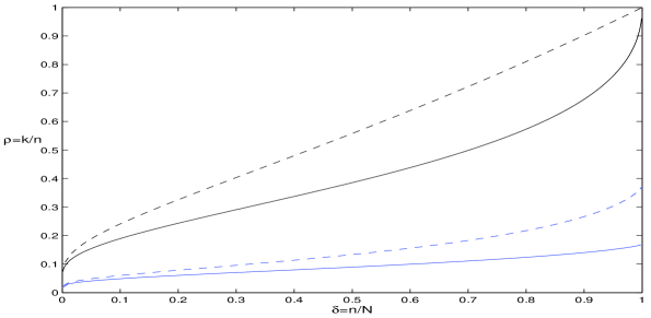
Figure 3.1. Weak thresholds for the simplex, $\rho_{W}(\delta;T^{N-1})$ (black-dash), and cross-polytope, $\rho_{W}(\delta;C^{N})$ (black-solid). Consider sequences obeying the proportional-dimensional asymptotic with parameters $\delta$, $\rho$. For $(\delta,\rho)$ below these curves, and for large $n$, each projected polytope has nearly as many $k$-faces as its generator; above these curves the projected polytope has noticeably fewer. Strong thresholds for the simplex, $\rho_{S}(\delta;T^{N-1})$ (blue-dash), and cross-polytope, $\rho_{S}(\delta;C^{N})$ (blue-solid). For $(\delta,\rho)$ below these curves, and for large $n$, each projected polytope and its generator typically have exactly the same number of $k$-faces.

3.2. Non-Existence of Strong Thresholds for Hypercube

Lemma 1.8 shows that projected zonotopes always have strictly fewer $k$-faces than their generators $f_{k}(AH^{N})<f_{k}(H^{N})$, for every $n<N$. this is again quite different from the situation with the simplex and the cross-polytope, where we can even have $n\ll N$ and still find $k$ for which $f_{k}(AQ)=f_{k}(Q)$, [13], see Figure 3.1.

3.3. Universality of weak phase transitions

For Theorems 1.1 and 1.5, $A$ can be sampled from any ensemble of random matrices having an orthant-symmetric and generic random null space. Our result is thus universal across a wide class of matrix ensembles.

In proving weak and strong threshold results for the simplex and cross-polytope, we required $A$ to either be a random ortho-projector or to have Gaussian iid entries. Thus, what we proved for those families of regular polytopes applies to a much more limited range of matrix ensembles than what has now been proven for hypercubes.

Our empirical studies suggest that the same ensembles of matrices which ‘work’ for the hypercube weak threshold also ‘work’ for the simplex and cross-polytope thresholds. It seems to us that the universality across matrix ensembles proven here may point to a much larger phenomenon, valid also for other polytope families. For our empirical studies see [14].

In fact, even in the hypercube case, the weak threshold phenomenon may be more general than what can be proven today; it seems also to hold for some matrix ensembles that may not have an orthant-symmetric null space.

4. Contrasting the Cone with the Hypercube

The weak Cone threshold depends very much more delicately on details about $A$ than do the hypercube thresholds; it really makes a difference to the results if the matrix $A$ is not ‘zero-mean’.

4.1. The Low-Frequency Partial Fourier Matrix

Consider the special partial Fourier matrix made only of the $n$ lowest frequency entries.

Corollary 4.1.

Assume $n$ is odd and let

(4.1) $$\Omega_{ij}=\left\{\begin{array}[]{ll}\cos\left(\frac{\pi(j-1)(i-1)}{N}\right)&i=1,3,5,\ldots,n\\ \sin\left(\frac{\pi(j-1)i}{N}\right)&i=2,4,6,\ldots,n-1.\end{array}\right.$$

Then

$$f_{k}(\Omega{\mathbb{R}}_{+}^{N})=f_{k}({\mathbb{R}}_{+}^{N}),\quad k=0,1,\dots,\frac{1}{2}(n-1).$$

This behavior is dramatically different than the case for random $A$ of the type considered so far, and in some sense dramatically better.

Corollary 4.1 is closely connected with the classical question of neighborliness. There are famous polytopes which can be generated by projections $AT^{N-1}$ and have exactly as many $k$-faces as $T^{N-1}$ for $k\leq\lfloor n/2\rfloor$. A standard example is provided by the matrix $\Omega$ defined in (4.1); it obeys $f_{k}(\Omega T^{N-1})=f_{k}(T^{N-1})$, $0\leq k\leq\lfloor n/2\rfloor$. (There is a vast literature touching in some way on the phenomenon $f_{k}(\Omega T^{N-1})=f_{k}(T^{N-1})$. In that literature, the polytope $\Omega T^{N-1}$ is usually called a cyclic polytope, and the columns of $\Omega$ are called points of the trigonometric moment curve; see standard references [16, 20]).

Hence the matrix $\Omega$ offers both $f_{k}(\Omega T^{N-1})=f_{k}(T^{N-1})$ and $f_{k}(\Omega{\mathbb{R}}_{+}^{N})=f_{k}({\mathbb{R}}_{+}^{N})$ for $0\leq k\leq\lfloor n/2\rfloor$. This is exceptional. For random $A$ of the type discussed in earlier sections, there is a large disparity between the sets of triples $(k,n,N)$ where $f_{k}(AT^{N-1})=f_{k}(T^{N-1})$ – this happens for $k/n<\rho_{S}(n/N;T^{N-1})$ – and those where $f_{k}(A{\mathbb{R}}_{+}^{N})=f_{k}({\mathbb{R}}_{+}^{N})$ – this happens for $k/n<\rho_{S}(n/N;{\mathbb{R}}_{+}^{N})$. These two strong thresholds are displayed in Figures 3.1 and 1.1 respectively.

Even if we relax our notion of agreement of face counts to weak agreement, the collections of triples where $f_{k}(AT^{N-1})\approx f_{k}(T^{N-1})$ and $f_{k}(A{\mathbb{R}}_{+}^{N})\approx f_{k}({\mathbb{R}}_{+}^{N})$ are very different, because the two curves $\rho_{W}(n/N;T^{N-1})$ and $\rho_{W}(n/N;{\mathbb{R}}_{+}^{N})$ are so dramatically different, particularly at $n<N/2$.

4.2. Adjoining a Row of Ones to $A$

An important feature of the random matrices $A$ studied earlier is that their random nullspace is orthant symmetric. In particular, the positive orthant plays no distinguished role with respect these matrices. On the other hand, the partial Fourier matrix $\Omega$ constructed in the last subsection contains a row of ones, and thus the positive orthant has a distinguished role to play for this matrix. Moreover, this distinction is crucial; we find empirically that removing the row of ones from $\Omega$ causes the conclusion of Corollary 4.1 to fail drastically.

Conversely, consider the matrix $\tilde{A}$ obtained by adjoining a row of $N$ ones to some matrix A:

$$\tilde{A}=\left[\begin{array}[]{l}1\\ A\end{array}\right].$$

Adding this row of ones to a random matrix causes a drastic shift in the strong and weak thresholds. The following is proved in Section 6.

Theorem 4.1.

Consider the proportional-dimensional asymptotic with parameters $\delta,\rho$ in $(0,1)$. Let the random $n-1$ by $N$ matrix $A$ have iid standard normal entries. Let $\tilde{A}$ denote the corresponding $n$ by $N$ matrix whose first row is all ones and whose remaining rows are identical to those of $A$. Then

(4.2) $$\lim_{n\rightarrow\infty}\frac{{\mathcal{E}}f_{k}(\tilde{A}{\mathbb{R}}_{+}^{N})}{f_{k}({\mathbb{R}}_{+}^{N})}=\left\{\begin{array}[]{cl}1,&\rho<\rho_{W}(\delta,T^{N-1})\\ <1,&\rho>\rho_{W}(\delta,T^{N-1})\end{array}\right..$$

(4.3) $$\lim_{n\rightarrow\infty}P\{f_{k}(\tilde{A}{\mathbb{R}}_{+}^{N})=f_{k}({\mathbb{R}}_{+}^{N})\}=\left\{\begin{array}[]{cl}1,&\rho<\rho_{S}(\delta,T^{N-1})\\ 0,&\rho>\rho_{S}(\delta,T^{N-1})\end{array}\right..$$

Note particularly the mixed form of this relationship. Although the conclusions concern the behavior of faces of the randomly-projected orthant, the thresholds are those that were previously obtained for the randomly-projected simplex.

Since there is such a dramatic difference between $\rho(\delta,T^{N-1})$ and $\rho(\delta,{\mathbb{R}}_{+}^{N})$, the single row of ones can fairly be said to have a huge effect. In particular, the region ’below’ the simplex weak phase transition $\rho_{W}(\delta,T^{N-1})$ comprises $\approx 0.5634$ of the $(\delta,\rho)$ parameter area, and the hypercube weak phase transition $\rho_{W}(\delta,H^{N})$ comprises $1-\log 2\approx 0.3069$.

5. Application: Compressed Sensing

Our face counting results can all be reinterpreted as statements about “simple” solutions of underdetermined systems of linear equations. This reinterpretation allows us to make connections with numerous problems of current interest in signal processing, information theory, and probability. The reinterpretation follows from the two following lemmas, which are restatements of Lemmas 2.2 and 2.5, rephrasing the notion of (Transverse($A,x_{0},Q$)) with the all but linguistically equivalent (Unique($A,x_{0},Q$)). For proofs of Lemmas 5.1 and 5.2 see the proofs of Lemmas 2.2 and 2.5.

Lemma 5.1.

Let $x_{0}$ be a vector in ${\mathbb{R}}_{+}^{N}$ with exactly $k$ nonzeros. Let $F$ denote the associated $k$-face of ${\mathbb{R}}_{+}^{N}$. For an $n\times N$ matrix $A$, let $AF$ denote the image of $F$ under $A$ and $b_{0}=Ax_{0}$ the image of $x_{0}$ under $A$. The following are equivalent:

(Survive($A,F,{\mathbb{R}}_{+}^{N}$)):	$AF$ is a $k$-face of $A{\mathbb{R}}_{+}^{N}$,
(Unique($A,x_{0},{\mathbb{R}}_{+}^{N}$)):	The system $b_{0}=Ax$ has a unique solution in ${\mathbb{R}}_{+}^{N}$.

Lemma 5.2.

Let $x_{0}$ be a vector in $H^{N}$ with exactly $k$ entries strictly between the bounds $\{0,1\}$. Let $F$ denote the associated $k$-face of $H^{N}$. For an $n\times N$ matrix $A$, let $AF$ denote the image of $F$ under $A$ and $b_{0}=Ax_{0}$ the image of $x_{0}$ under $A$. The following are equivalent:

(Survive($A,F,H^{N}$)):	$AF$ is a $k$-face of $AH^{N}$,
(Unique($A,x_{0},H^{N}$)):	The system $b_{0}=Ax$ has a unique solution in $H^{N}$.

Note that the systems of linear equations referred to in these lemmas are underdetermined: $n<N$. Hence these lemmas identify conditions on underdetermined system of linear equations, such that, when the solution is known to obey certain constraints, there are many cases where this seemingly weak a priori knowledge in fact uniquely determines the solution. The first result can be paraphrased as saying that nonnegativity constraints can be very powerful, if the object is known to have relatively few nonzeros; the second result says that upper and lower bounds can be very powerful, provided those bounds are active in most cases.

These results provide a theoretical vantage point on an area of recent intense interest in signal processing, appearing variously under the labels “Compressed Sensing” or “Compressive Sampling”.

In many practical applications of scientific and engineering signal processing – spectroscopy is one example – one can obtain $n$ linear measurements of an object $x$, obtaining data $b=Ax$; here the rows of the matrix $A$ give the linear response functions of the measurement devices. We wish to reconstruct $x$, knowing only the measurements $b$, the measurement matrix $A$, and various a͡ priori constraints on $x$.

It could be very useful to be able to do this in the case $n<N$, allowing us to save measurement time or other resources. This seems hopeless, because the linear system is underdetermined; but the above lemmas show that there is some fundamental soundness to the idea that we can have $n<N$ and still reconstruct. We now spell out the consequences of these lemmas in more detail.

5.1. Reconstruction Exploiting Nonnegativity Constraints

Many practical applications, such as spectroscopy and astronomy, the object $x$ to be recovered is known a priori to be nonnegative. We wish to reconstruct the unknown $x$, knowing only the linear measurements $b=Ax$, the matrix $A$, and the constraint $x\in{\mathbb{R}}_{+}^{N}$.

Let $J(x)$ be some function of $x$. Consider the positivity-constrained variational problem

$$(Pos_{J})\qquad\min J(x)\qquad\mbox{ subject to }b=Ax,\qquad x\in{\mathbb{R}}_{+}^{N}.$$

Let $pos_{J}(b,A)$ denote any solution of the problem instance $(Pos_{J})$ defined by data $b$ and matrix $A$.

Typical variational functions $J$ include

• Sparsity: $\|x\|_{\ell^{0}}:=\#\{i:x>0\}$.

• Size: $1^{\prime}x$.

• negEntropy: $\sum x(j)\log(x(j))$

• Energy: $\sum x(j)^{2}$

This framework contains as special cases the popular signal processing methods of maximum entropy reconstruction and nonnegative least-squares reconstruction.

We conclude the following:

Corollary 5.1.

Suppose that

$$f_{k}(A{\mathbb{R}}_{+}^{N})=f_{k}({\mathbb{R}}_{+}^{N}).$$

Let $x_{0}\geq 0$ and $\|x_{0}\|_{\ell^{0}}\leq k$. For the problem instance defined by $b=Ax_{0}$

$$pos_{J}(b,A)=x_{0}.$$

In words: under the given conditions on the face numbers, any variational prescription which imposes nonnegativity constraints will correctly recover the $k$-sparse solution in any problem instance where such a $k$-sparse solution exists. This may seem surprising; as $n<N$, the system of linear equations is underdetermined yet we correctly find a sparse solution if it exists.

Corresponding to this ‘strong’ statement is a ‘weak’ statement. Consider the following probability measure on $k$-sparse problem instances.

• Choose a random subset $I$ of size $k$ from $\{1,\dots,N\}$, by $k$ simple random draws without replacement.

• Set the entries of $x_{0}$ not in the selected subset to zero.

• Choose the entries of $x_{0}$ in the selected set $I$ from some fixed joint distribution $\psi_{I}$ supported in $(0,1)^{k}$.

• Generate the problem instance $b=Ax_{0}$.

We speak of drawing a $k$-sparse random problem instance at random.

Corollary 5.2.

Suppose that for some $\epsilon\in(0,1)$.

$$f_{k}(A{\mathbb{R}}_{+}^{N})\geq(1-\epsilon)\cdot f_{k}({\mathbb{R}}_{+}^{N}).$$

For $(b,A)$ a problem instance drawn at random, as above:

$$\mbox{Prob}\{pos_{J}(b,A)=x_{0}\}\geq(1-\epsilon).$$

In words: under the given conditions on the face lattice, any variational prescription which imposes nonnegativity constraints will correctly succeed to recover the $k$-sparse solution in at least a fraction $(1-\epsilon)$ of all $k$-sparse problem instances. This may seem surprising; since $n<N$, the system of linear equations is underdetermined, and yet, we typically find a sparse solution if it exists.

Here are some simple applications:

• In the proportional-dimensional framework, consider triples $(k_{n},n,N_{n})$ with parameters $\delta,\rho$. Let $A$ denote an $n$ by $N_{n}$ matrix having random nullspace which is orthant symmetric and generic.

  • If the parameters $\delta,\rho$ name a point ’below’ the orthant weak threshold $\rho_{W}(\delta;{\mathbb{R}}_{+}^{N})$, then for the vast majority of $k_{n}$-sparse vectors, any variational method will correctly recover the vector.

  • If the parameters $\delta,\rho$ name a point ’below’ the orthant strong threshold $\rho_{S}(\delta;{\mathbb{R}}_{+}^{N})$, then for large enough $n$, every $k_{n}$-sparse vector can be correctly recovered by any variational method imposing positivity constraints.

• In the proportional-dimensional asymptotic, consider triples $(k_{n},n,N_{n})$ with parameters $\delta,\rho$. Let $A_{0}$ denote an $n-1$ by $N_{n}$ matrix having iid standard normal entries. And let $A$ denote the $n$ by $N_{n}$ matrix formed by adjoining a row of ones to $A_{0}$.

  • If the parameters $\delta,\rho$ name a point ’below’ the simplex weak threshold $\rho_{W}(\delta;T^{N-1})$, then for the vast majority of $k_{n}$-sparse vectors, any variational method will correctly recover the sparse vector.

  • If the parameters $\delta,\rho$ name a point ’below’ the simplex strong threshold $\rho_{S}(\delta,T^{N-1})$, then for large enough $n$, every $k_{n}$-sparse vector can be correctly recovered by any variational method imposing positivity constraints.

• Let $A$ denote the $n$ by $N$ partial Fourier matrix built from low frequencies and called $\Omega$ in Section 4.1. Every $\lfloor n/2\rfloor$-sparse vector will be correctly recovered by any variational method imposing positivity constraints.

Hence in positivity-constrained reconstruction problems where the object to be recovered is zero in most entries – an assumption which approximates the truth in many problems of spectroscopy and astronomical imaging [9], we can work with fewer than $N$ samples. The above paragraphs show that it matters a great deal what matrix $A$ we use. Our preference order:

$\Omega$ is better than the random matrix, $\tilde{A}$ is better than a random zero-mean matrix $A$.

(These results extend and generalize results which were previously obtained by the authors in [11], in the case where $J(x)=1^{\prime}x$, and by the first author and coauthors in [9]; see also Fuchs [15] and Bruckstein, Elad, and Ziubulevsky [6].)

5.2. Reconstruction Exploiting Box Constraints

Consider again the problem of reconstruction from measurements $b=Ax$, but this time assuming the object $x$ obeys box-constraints: $0\leq x(j)\leq 1$, $1\leq j\leq N$. Such constraints can arise for example in infrared absorption spectroscopy and in binary digital communications.

We define the box-constrained variational problem

$$(Box_{J})\qquad\min J(x)\qquad\mbox{ subject to }b=Ax,\qquad 0\leq x(j)\leq 1,\quad j=1,\dots,N.$$

Let $box_{J}(b,A)$ denote any solution of the problem instance $(Box_{J})$ defined by data $b$ and matrix $A$.

In this setting, the notion corresponding to ’sparse’ is ’simple’. We say that a vector $x$ is $k$-simple if at most $k$ of its entries differ from the bounds $\{0,1\}$. Here, the interesting functions $J$ penalize deviations from simple structure; they include:

• Simplicity: $\#\{i:x(i)\not\in\{0,1\}\}$.

• Violation Energy: $\sum x(j)(1-x(j))$

Corollary 5.3.

Suppose that

$$f_{k}(AH^{N})=f_{k}(H^{N}).$$

Let $x_{0}$ be a $k$-simple vector obeying the box constraints $0\leq x_{0}\leq 1$. For the problem instance defined by $b=Ax_{0}$,

$$box_{J}(b,A)=x_{0}.$$

In words: under the given conditions on the face lattice, any variational prescription which imposes box constraints, when presented with a problem instance where there is a $k$-simple solution, will correctly recover the $k$-simple solution.

Corresponding to this ‘strong’ statement is a ‘weak’ statement. Consider the following probability measure on problem instances having $k$-simple solutions. Recall that $k$-simple vectors have all entries equal to $0$ or $1$ except at $k$ exceptional locations.

• Choose the subset $I$ of $k$ exceptional entries uniformly at random from the set $\{1,\dots,N\}$ without replacement;

• Choose the nonexceptional entries to be either $0$ or $1$ based on tossing a fair coin.

• Choose the values of the exceptional $k$ entries according to a joint probability measure $\psi_{I}$ supported in $(0,1)^{k}$.

• Define the problem instance $b=Ax_{0}$.

Corollary 5.4.

Suppose that for some $\epsilon\in(0,1)$.

$$f_{k}(AH^{N})\geq(1-\epsilon)\cdot f_{k}(H^{N}).$$

Randomly sample a problem instance $(b,A)$ using the method just described.

$$P\{box_{J}(b,A)=x_{0}\}\geq(1-\epsilon).$$

In words: under the given conditions on the face lattice, any variational prescription which imposes box constraints will correctly recover at least a fraction $(1-\epsilon)$ of all underdetermined systems generated by the matrix $A$ which have $k$-simple solutions.

Here is a simple application. In the proportional-dimensional asymptotic framework, consider triples $(k_{n},n,N_{n})$ with parameters $\delta,\rho$. Let $A$ denote an $n$ by $N_{n}$ matrix having random nullspace which is orthant symmetric and generic. If the parameters $\delta,\rho$ name a point ’below’ the hypercube weak threshold, then for the vast majority of $k_{n}$-simple vectors, any variational method imposing box constraints will correctly recover the vector.

In the hypercube case, to our knowledge, there is no phenomenon comparable to that which arose in the positive orthant with the special constructions $\Omega$ and $\tilde{A}$.

Consequently, the hypercube weak threshold is the best known general result on the ability to undersample by exploiting box constraints. In particular, the difference between the weak simplex threshold and the weak hypercube threshold has this interpretation:

A given degree $k$ of sparsity of a nonnegative object is much more powerful than that same degree simplicity of a box-constrained object.

Specifically, we shouldn’t expect to be able to undersample a typical box-constrained object by more than a factor of $2$ and then reconstruct it using some garden-variety variational prescription. In comparison, the last section showed that we can severely undersample very sparse nonnegative objects.

Because box constraints are of interest in important areas of signal processing, it seems that much more attention should be paid to thresholds associated with the hypercube.

6. Additional Proofs

6.1. Proof of Lemma 2.2

Let $b_{0}:=Ax_{0}$.

Assume (Survive($A,F,{\mathbb{R}}^{N}_{+}$)), that $AF$ is a $k$-face of $A{\mathbb{R}}^{N}_{+}$. General position of $A$ implies that $AF$ is a simplicial cone of dimension $k-1$, and that there exists a unique $x\in{\mathbb{R}}^{N}_{+}$ satisfying $Ax=b_{0}$, with $x_{0}$ being that solution. We now assume $\exists\;\nu\in{\mathcal{N}}(A)\cap Feas_{x_{0}}({\mathbb{R}}^{N}_{+})\neq 0$. Then $\exists\;\epsilon>0$ small enough such that $z_{0}:=x_{0}+\epsilon\nu\in{\mathbb{R}}^{N}_{+}$. This $z_{0}$ satisfies $Az_{0}=b_{0}$, in contradiction to the uniqueness condition previously stated, therefor ${\mathcal{N}}(A)\cap Feas_{x_{0}}({\mathbb{R}}^{N}_{+})=\{0\}$.

For the converse direction, assume (Transverse($A,x_{0},{\mathbb{R}}^{N}_{+}$)), that ${\mathcal{N}}(A)\cap Feas_{x_{0}}({\mathbb{R}}^{N}_{+})=\{0\}$. Assume $AF$ is not a $k$-face of $A{\mathbb{R}}^{N}_{+}$, that is $AF$ is interior to $A{\mathbb{R}}^{N}_{+}$. As $A$ projects the interior of ${\mathbb{R}}^{N}_{+}$ to the complete interior of $A{\mathbb{R}}^{N}_{+}$, $\exists\;z_{0}\in{\mathbb{R}}^{N}_{+}$ with $z_{0}>0$ with $Az_{0}=b_{0}$. The difference $\nu:=z_{0}-x_{0}\neq 0$, but $\nu\in{\mathcal{N}}(A)\cap Feas_{x_{0}}({\mathbb{R}}^{N}_{+})$ contradicting the Transverse assumption, implying $AF$ is a $k$-face of $A{\mathbb{R}}^{N}_{+}$.

∎

6.2. Proof of Lemma 2.5

This proof follows similarly to that of Lemma 2.2 and is omitted.

6.3. Proof of Lemma 2.6

For points $x_{0}$ on $k$-faces of $H^{N}$ that are also $k$-faces of ${\mathbb{R}}_{+}^{N}$ they share the same feasible set

$$Feas_{x_{0}}(H^{N})=Feas_{x_{0}}({\mathbb{R}}_{+}^{N})$$

and by Lemmas 2.2 and 2.5 the probabilities of (Survive($A,F,Q$)) for $Q={\mathbb{R}}_{+}^{N},H^{N}$ must be equal. Consider a point $x_{0}$ on a $k$-face of $H^{N}$ that is not a $k$-face of ${\mathbb{R}}_{+}^{N}$; without loss of generality, due to column exchangeability, let

$$x_{0}(i)=\left\{\begin{array}[]{cl}0&i=1,\ldots,\ell\\ 1&i=\ell+1,\ldots,N-k\\ 1/2&i=N-k+1,\ldots N\end{array}\right.$$

Then Feas${}_{x_{0}}(H^{N})=\{\nu:\nu_{1},\ldots,\nu_{\ell}\geq 0,\nu_{\ell+1},\ldots,\nu_{N-k}\leq 0\}$. Following the proof of Lemma 2.3, condition (Transverse($A,x_{0},H^{N}$)) can be restated as

(6.1) $$(\mbox{Ineq }H^{N})\quad\left\{\begin{array}[]{l}\mbox{The only vector }c\mbox{ satisfying}\\ (B^{T}c)_{i}\geq 0,\quad i=1,\ldots,\ell,\\ (B^{T}c)_{i}\leq 0,\quad i=\ell+1,\ldots,N-k,\\ \mbox{is the vector }c=0\end{array}\right.$$

where $B$ is the orthogonal complement of $A$.

Orthant symmetry of $B$ states that the sign of $(B^{T}c)_{i}$ is equiprobable; consequently, the probability of the event named (6.1) is independent of $\ell$, and is in fact equal to the probability of the event named in (2.3).

∎

6.4. Proof of Corollary 4.1

The result is a corollary of [9, Theorem 3, pp. 56]. However, it may require effort on the part of readers to see this, so we select the key step from the proof of Theorem 3, [9, Lemma 2, pp. 63], and use it directly within the framework of this paper.

As $n$ is odd, write $n=2m+1$ where $m$ is an integer. The range of the matrix $\Omega$ is the span of all Fourier frequencies from 0 to $\pi(m-1)/N$. In accord with terminology in electrical engineering, this space of vectors with be called the space of Lowpass sequences ${\mathcal{L}}(m)$. The nullspace of $\Omega$ is the span of all Fourier frequencies from $\pi m/N$ to $\pi/N$. It will be called the space of Highpass sequences ${\mathcal{H}}(m)$.

We have the following:

Lemma 6.1.

[9] Every sequence in ${\mathcal{H}}(m)$ has at least $m$ negative entries.

Recall condition $(\mbox{Transverse}(\Omega,x_{0},{\mathbb{R}}_{+}^{N}))$. If $x_{0}$ has $k$ nonzeros, then vectors in $Feas_{x_{0}}({\mathbb{R}}_{+}^{N})$ have at most $k$ negative entries. But vectors in ${\mathcal{N}}(\Omega)={\mathcal{H}}(m)$ have at least $m$ negative entries. Therefore, if $m>k$, $(\mbox{Transverse}(\Omega,x_{0},{\mathbb{R}}_{+}^{N}))$ must hold.

By Lemma 2.2, every $(\mbox{Survive}(\Omega,F,{\mathbb{R}}_{+}^{N}))$ must hold for every $k$-face with $k<m$. Hence $f_{k-1}(\Omega{\mathbb{R}}_{+}^{N})=f_{k-1}({\mathbb{R}}_{+}^{N})$, for $k\leq m=\frac{1}{2}(n-1)$. ∎

6.5. Proof of Theorem 4.1

The Theorem is an immediate consequence of the following identity.

Lemma 6.2.

Suppose that the row vector $1$ is not in the row span of $A$. Then

$$f_{k}(\tilde{A}{\mathbb{R}}_{+}^{N})=f_{k-1}(AT^{N-1}),0<k<n.$$

Proof.

We observe that there is a natural bijection between $k$-faces of ${\mathbb{R}}_{+}^{N}$ and the $k-1$-faces of $T^{N-1}$. The $k-1$-faces of $T^{N-1}$ are in bijection with the corresponding support sets of cardinality $k$: i.e. we can identify with each $k$-face $F$ the union $I$ of all supports of all members of the face. Similarly to each support set $I$ of cardinality $k$ there is a unique $k$-face $\tilde{F}$ of ${\mathbb{R}}_{+}^{N}$ consisting of all points in ${\mathbb{R}}_{+}^{N}$ whose support lies in $I$. Composing bijections $F\leftrightarrow I\leftrightarrow\tilde{F}$ we have the bijection $F\leftrightarrow\tilde{F}$.

Concretely, let $x_{0}$ be a point in the relative interior of some $k-1$-face $F$ of $T^{N-1}$. Then $x_{0}$ has $k$ nonzeros. $x_{0}$ is also in the relative interior of the $k$-face $\tilde{F}$ of ${\mathbb{R}}_{+}^{N}$ Conversely, let $y_{0}$ be a point in the relative interior of some $k$-face of ${\mathbb{R}}_{+}^{N}$; then $x_{0}=(1^{\prime}y_{0})^{-1}y_{0}$ is a point in the relative interior of a $k-1$-face of $T^{N-1}$.

The last two paragraphs show that for each pair of corresponding faces $(F,\tilde{F})$, we may find a point $x_{0}$ in both the relative interior of $\tilde{F}$ and also of the relative interior of $F$. For such $x_{0}$,

$$\mbox{Feas}_{x_{0}}({\mathbb{R}}_{+}^{N})=\mbox{Feas}_{x_{0}}(T^{N-1})+lin(x_{0}).$$

Clearly ${\mathcal{N}}(\tilde{A})\cap lin(x_{0})=\{0\}$, because $1^{\prime}x_{0}>0$. We conclude that the following are equivalent:

(Transverse($A,x_{0},T^{N-1}$))	${\mathcal{N}}(A)\cap\mbox{Feas}_{x_{0}}(T^{N-1})=\{0\}$.
(Transverse($\tilde{A},x_{0},{\mathbb{R}}_{+}^{N}$))	${\mathcal{N}}(\tilde{A})\cap\mbox{Feas}_{x_{0}}({\mathbb{R}}_{+}^{N})=\{0\}$.

Rephrasing [11], the following are equivalent for $x_{0}$ a point in the relative interior of $F$:

(Survive($A,F,T^{N-1}$))	$AF$ is a $k-1$-face of $AT^{N-1}$,
(Transverse($A,x_{0},T^{N-1}$))	${\mathcal{N}}(A)\cap\mbox{Feas}_{x_{0}}(T^{N-1})=\{0\}$.

We conclude that for two corresponding faces $F$, $\tilde{F}$, the following are equivalent:

(Survive($A,F,T^{N-1}$)):	$AF$ is a $k-1$-face of $AT^{N-1}$,
(Survive($\tilde{A},\tilde{F},{\mathbb{R}}_{+}^{N}$)):	$\tilde{A}\tilde{F}$ is a $k$-face of $\tilde{A}{\mathbb{R}}_{+}^{N}$ .

Combining this with the natural bijection $F\leftrightarrow\tilde{F}$, the lemma is proved. ∎

Acknowledgments.

Art Owen suggested that we pay attention to Wendel’s Theorem. We also thank Goodman, Pollack, and Schneider for providing scholarly background.

References

- [1] Fernando Affentranger and Rolf Schneider, Random projections of regular simplices, Discrete Comput. Geom. 7 (1992), no. 3, 219–226. MR MR1149653 (92k:52008)
- [2] Yuliy M. Baryshnikov, Gaussian samples, regular simplices, and exchangeability, Discrete Comput. Geom. 17 (1997), no. 3, 257–261. MR MR1432063 (98a:52006)
- [3] Yuliy M. Baryshnikov and Richard A. Vitale, Regular simplices and Gaussian samples, Discrete Comput. Geom. 11 (1994), no. 2, 141–147. MR MR1254086 (94j:60017)
- [4] Ethan D. Bolker, A class of convex bodies, Trans. Amer. Math. Soc. 145 (1969), 323–345. MR MR0256265 (41 #921)
- [5] Károly Böröczky, Jr. and Martin Henk, Random projections of regular polytopes, Arch. Math. (Basel) 73 (1999), no. 6, 465–473. MR MR1725183 (2001b:52004)
- [6] A. M. Bruckstein, M. Elad, and M. Zibulevsky, On the uniqueness of non-negative sparse and redundant representations, ICASSP 2008 special session on Compressed Sensing, Las Vegas, Nevada., 2008.
- [7] David L. Donoho, High-dimensional centrally-symmetric polytopes with neighborliness proportional to dimension, Disc. Comput. Geometry 35 (2006), no. 4, 617–652.
- [8] by same author, Neighborly polytopes and sparse solutions of underdetermined linear equations, Stanford University, Technical Report (2006).
- [9] David L. Donoho, Iain M. Johnstone, Jeffrey C. Hoch, and Alan S. Stern, Maximum entropy and the nearly black object, Journal of the Royal Statistical Society, Series B (Methodological) 54 (1992), no. 1, 41–81.
- [10] David L. Donoho and Jared Tanner, Neighborliness of randomly-projected simplices in high dimensions, Proc. Natl. Acad. Sci. USA 102 (2005), no. 27, 9452–9457.
- [11] by same author, Sparse nonnegative solutions of underdetermined linear equations by linear programming, Proc. Natl. Acad. Sci. USA 102 (2005), no. 27, 9446–9451.
- [12] by same author, Exponential bounds implying construction of neighborly polytopes, error-correcting codes and compressed sensing matrices by random sampling, preprint (2007).
- [13] by same author, Counting faces of randomly-projected polytopes when the projection radically lowers dimension, J. AMS (2008).
- [14] by same author, Sharp thresholds in compressed sensing are universal across matrix ensembles, (2008).
- [15] Jean-Jacques Fuchs, On sparse representations in arbitrary redundant bases, IEEE Trans. Inform. Theory 50 (2004), no. 6, 1341–1344. MR MR2094894
- [16] Branko Grünbaum, Convex polytopes, second ed., Graduate Texts in Mathematics, vol. 221, Springer-Verlag, New York, 2003, Prepared and with a preface by Volker Kaibel, Victor Klee and Günter M. Ziegler. MR MR1976856
- [17] Mark Rudelson and Roman Vershynin, The smallest singular value of a rectangular random matrix, preprint (2008).
- [18] A. M. Vershik and P. V. Sporyshev, Asymptotic behavior of the number of faces of random polyhedra and the neighborliness problem, Selecta Math. Soviet. 11 (1992), no. 2, 181–201. MR MR1166627 (93d:60017)
- [19] James G. Wendel, A problem in geometric probability, Mathematics Scandinavia 11 (1962), 109–111.
- [20] Günter M. Ziegler, Lectures on polytopes, Graduate Texts in Mathematics, vol. 152, Springer-Verlag, New York, 1995. MR MR1311028 (96a:52011)