Apparent and average acceleration of the Universe

Abstract

In this paper we consider the relation between the volume deceleration parameter obtained within the Buchert averaging scheme and the deceleration parameter derived from the supernova observation. This work was motivated by recent findings that showed that there are models which despite $\Lambda=0$ have volume deceleration parameter $q^{vol}<0$. This opens the possibility that backreaction and averaging effects may be used as an interesting alternative explanation to the dark energy phenomenon.

We have calculated $q^{vol}$ in some Lemaître–Tolman models. For those models which are chosen to be realistic and which fit the supernova data, we find that $q^{vol}>0$, while those models which we have been able to find which exhibit $q^{vol}<0$ turn out to be unrealistic. This indicates that care must be exercised in relating the deceleration parameter to observations.

Keywords: dark energy theory, supernova type Ia, superclusters and voids

1 Introduction

Accelerated expansion, modeled by a positive cosmological constant, is an essential element of the current standard cosmological model of the Universe. The accelerated expansion was originally motivated by supernova observations [1] and is supported by many other types of cosmological observations. Observational data is, in modern cosmology, analyzed almost exclusively within the framework of homogeneous and isotropic Friedmann models [2]. This analysis leads to the Concordance model, which provides a remarkably precise fit to cosmological observations. In this situation, if the Ehlers-Geren-Sachs theorem [3] and ‘almost EGS theorem’ [4] are invoked, then it seems that an assumption of large scale homogeneity of the Universe can be justified. This on the other hand implies that the Universe must be filled with dark energy which currently drives the acceleration of the Universe.

However the Concordance model is not the only one which can fit cosmological observations. Anti-Copernican inhomogeneous models which assume the existence of a local Gpc scale void also fit cosmological observations [6] (see [7] for a review). Moreover, on small and medium scales our Universe is not homogeneous. Therefore, one may ask whether Friedmann models can describe our Universe correctly. In particular, it is important to ask what is the best way to fit a homogeneous model to a realistic and inhomogeneous Universe. This problem, known as the fitting problem, was considered by Ellis and Stoeger [8]. In considering the fitting problem, it becomes apparent that a homogeneous model fitted to inhomogeneous data can evolve quite differently from the real Universe. The difference between evolution of homogeneous models and an inhomogeneous Universe is caused by backreaction effects, due to the nonlinearity of the Einstein equation. Unfortunately, in the standard approach, the backreaction is rarely taken into account – in most cases when modelling our Universe on a local scale Newtonian mechanics is employed and on large scales the Friedmann equations (or linear perturbations of Friedmann background) are used [9]. Such an approach to cosmology is often encouraged by the “no–go” theorem which states that the Universe can be very accurately described by the conformal Newtonian metric perturbed about a spatially flat background, even if $\delta\rho/\rho\gg 0$. In such a case the backreaction is negligible [10, 11]. However, the results obtained by van Elst and Ellis [12] and recently by Kolb, Marra and Matarrese [13] show that the application of “no-go” theorem is limited. Therefore, one should be aware that in the absence of an analysis of the backreaction and other effects caused by inhomogeneities in the universe, there remains the possibility that the observed accelerated expansion of the Universe is only apparent [14]. The direct study of the dynamical effects of inhomogeneities is difficult. Due to the nonlinearity of the Einstein equations, the solution of the Einstein equations for the homogeneous matter distribution leads in principle to a different description of the Universe than an average of a inhomogeneous solution to the exact Einstein equations (even though inhomogeneities when averaged over a sufficiently large scale might tend to be zero).

Neither the analysis of the evolution of a general matter distribution nor the numerical evolution of cosmological models employing the full Einstein equations are available at the level of detail which would make them useful for this problem. There are currently several different approaches which attempt to take backreaction effects into account. One approach is based on exact solutions – see for example [15]. Another, and more popular approach is based on averaging.

In the averaging approach to backreaction, one considers a solution to the Einstein equations for a general matter distribution and then an average of various observable quantities is taken. If a simple volume average is considered then such an attempt leads to the Buchert equations [16]. The Buchert equations are very similar to the Friedmann equations except for the backreaction term which is in general nonvanishing, if inhomogeneities are present. For a review on backreaction and the Buchert averaging scheme the reader is referred to [17, 18]. Within this framework and using spherically symmetric inhomogeneous models Nambu and Tanimoto [19], Paranjape and Singh [20], Kai, Kozaki, Nakao, Nambu, and Yoo [21], Chuang, Gu, and Hwang [22], provided explicit examples that one can obtain negative values of the volume deceleration parameter even if $\Lambda=0$. Another interesting example was presented by Räsänen [17, 23] where it was shown that the total volume deceleration parameter of two isolated and locally decelerating regions can also be negative.

There are however important ambiguities in the application of an averaging procedure. The average itself not only depends on a choice of volume but also on a choice of time slicing. This is very crucial in cosmology. Once inhomogeneities are present the age of the Universe is not everywhere the same. Namely, the big bang in inhomogeneous models is not a single event, so the average taken over a hypersurface of constant cosmic time $t$ is different from the average taken over a hypersurface of constant age of the Universe $t-t_{B}$ [24]. Moreover, the results of the averaging procedure vary if the discrepancy between the average cosmic time and the local time is introduced (the local time is the time which is measured by local clocks; the cosmic time is the time which appears in the averaged homogeneous model). This phenomenon was studied by Wiltshire [25], and has been used in an ambitious alternative concordance model. The model proposed by Wiltshire introduces some additional assumptions which allow to some extent a comparison of averaged quantities with observations. Such a comparison shows quite good agreement with observations, [26]. Thus, while serious fundamental questions remain concerning Wiltshire’s approach, it is another example of an approach where one does not need dark energy to fit cosmological observations.

The averaging procedure is also gauge-dependent. For example using different gauge one can obtain that the backreaction mimics not dark energy but dark matter [27]. The averaging schemes, therefore, in the literature have been criticized, and their inherent ambiguities (and in some cases obscurity) have been discussed, cf. e.g. [10]. A key point is that it is far from obvious if the average quantities, such as the acceleration of the averaged universe are really the quantities which are measured in astronomical observations. In particular, an operational analysis is to a large extent lacking in the discussions of averaging. Thus, it is important to test the averaging procedures with the exact and inhomogeneous solutions of the Einstein equations. Within exact models each quantity can easily be calculated and then compared with its averaged counterpart. This paper aims to perform such an analysis within the Lemaître–Tolman model.

The structure of this paper is as follows. Buchert’s averaging procedure is presented in section 2, and some background on the Lemaître–Tolman model is given in section 3. The volume and distance deceleration parameters are introduced in section 4. Finally, in section 5, we discuss the relation between the deceleration parameters, supernova observations and models of cosmic structures.

2 The Buchert scheme

If the averaging procedure is applied to the Einstein equations, then for irrotational and pressureless matter the following equations are obtained [16]

$$3\frac{\ddot{a}}{a}=-4\pi G\langle{\rho}\rangle+\mathcal{Q},$$ (1)

$$3\frac{\dot{a}^{2}}{a^{2}}=8\pi G\langle{\rho}\rangle-\frac{1}{2}\langle{\mathcal{R}}\rangle-\frac{1}{2}\mathcal{Q},$$ (2)

$$\mathcal{Q}\equiv\frac{2}{3}\left(\langle{{\Theta^{2}}}\rangle-\langle{\Theta}\rangle^{2}\right)-2\langle{\sigma^{2}}\rangle,$$ (3)

where $\langle{\mathcal{R}}\rangle$ is an average of the spacial Ricci scalar ${}^{(3)}\mathcal{R}$, $\Theta$ is the scalar of expansion, $\sigma$ is the shear scalar, and $\langle{\ }\rangle$ is the volume average over the hypersurface of constant time: $\langle{A}\rangle=(\int d^{3}x\sqrt{-h})^{-1}\int d^{3}x\sqrt{-h}A$. The scale factor $a$ is defined as follows:

$$a=(V/V_{0})^{1/3},$$ (4)

where V₀ is an initial volume.

Equations (1) and (2) are very similar to the Friedmann equations, where Q=0, and $\rho$ and $\mathcal{R}$ depend on time only. In fact, they are kinematically equivalent with a Friedmann model that has an additional scalar field source [28]. However the Buchert equation do not form a closed system. To close these equation one has to introduce some further assumptions [16]. As can be seen from (3) if the dispersion of expansion is large, Q can be large as well and one can get acceleration ($\ddot{a}>0$) without employing the cosmological constant.

3 The Lemaître–Tolman model

The Lemaître–Tolman model [30] is a spherical symmetric, pressure free and irrotational solution of the Einstein equations. Its metric is of the following form

$${\rm d}s^{2}=c^{2}{\rm d}t^{2}-\frac{R^{\prime 2}(r,t)}{1+2E(r)}\ {\rm d}r^{2}-R^{2}(t,r){\rm d}\Omega^{2},$$ (5)

where ${\rm d}\Omega^{2}={\rm d}\theta^{2}+\sin^{2}\theta{\rm d}\phi^{2}$. Because of the signature $(+,-,-,-)$, the $E(r)$ function must obey $E(r)\geq-1/2.$ Prime ^′ denotes $\partial_{r}$.

The Einstein equations reduce, in $\Lambda=0$ case, to the following two

$$\kappa\rho(r,t)c^{2}=\frac{2M^{\prime}(r)}{R^{2}(r,t)R^{\prime}(r,t)},$$ (6)

$$\frac{1}{c^{2}}\dot{R}^{2}(r,t)=2E(r)+\frac{2M(r)}{R(r,t)},$$ (7)

where $M(r)$ is another arbitrary function and $\kappa=8\pi G/c^{4}$. Dot $\dot{}$ denotes $\partial_{t}$.

When $R^{\prime}=0$ and $M^{\prime}\neq 0$, the density becomes infinite. This happens at shell crossings. This is an additional singularity to the Big Bang that occurs at $R=0,M^{\prime}\neq 0$. By setting the initial conditions appropriately the shell crossing singularity can be avoided (see [31] for detail discussion).

Equation (7) can be solved by simple integration:

$$\int\limits_{0}^{R}\frac{d\tilde{R}}{\sqrt{2E+\frac{2M}{\tilde{R}}}}=c\left[t-t_{B}(r)\right],$$ (8)

where $t_{B}$ appears as an integration constant and is an arbitrary function of $r$. This means that the big bang is not a single event as in the Friedmann models, but occurs at different times at different distances from the origin.

The scalar of the expansion is equal to

$$\Theta=\frac{\dot{R}^{\prime}}{R^{\prime}}+2\frac{\dot{R}}{R}.$$ (9)

The shear tensor is of the following form:

$$\sigma^{\alpha}{}_{\beta}=\frac{1}{3}\left(\frac{\dot{R}^{\prime}}{R^{\prime}}-\frac{\dot{R}}{R}\right){\rm diag}(0,2,-1,-1),$$ (10)

thus $\sigma^{2}\equiv(1/2)\sigma_{\alpha\beta}\sigma^{\alpha\beta}=(1/3)(\dot{R}^{\prime}/R^{\prime}-\dot{R}/R)^{2}$.

The spacial Ricci scalar in the Lemaître–Tolman is equal to

$${}^{(3)}\mathcal{R}=-\frac{4}{R^{2}}\left(E+\frac{E^{\prime}R}{R^{\prime}}\right)$$ (11)

4 The apparent and average acceleration

The deceleration parameter within the Friedmann models is defined as

$$q=-\frac{\ddot{a}a}{\dot{a}^{2}},$$ (12)

where $a$ is the scale factor. By analogy we can define the deceleration parameter which is based on the averaging scheme. Substituting (4) into (12) and using (1) and (2) we get

$$q^{vol}=-\frac{-4\pi G\langle{\rho}\rangle+\mathcal{Q}}{8\pi G\langle{\rho}\rangle-\frac{1}{2}\langle{\mathcal{R}}\rangle-\frac{1}{2}\mathcal{Q}}.$$ (13)

We refer to this deceleration parameter as the volume deceleration parameter, $q^{vol}$ since it is positive when the second derivative of volume is negative and negative when the second derivative of volume is positive (and of sufficiently large value).

On the other hand one can introduce a deceleration parameter defined relative to the distance. Within homogeneous models the distance to a given redshift is larger for accelerating models than for decelerating ones. Taylor expanding the luminosity distance in the Friedmann model we obtain

$$D_{L}=\left.\frac{dD_{L}}{dz}\right|_{z=0}z+\frac{1}{2}\left.\frac{d^{2}D_{L}}{dz^{2}}\right|_{z=0}z^{2}+\mathcal{O}(z^{3})$$

$$=\frac{c}{H_{0}}z+\frac{c}{2H_{0}}(1-q)z^{2}+\mathcal{O}(z^{3}).$$ (14)

Employing a similar procedure in the case of the Lemaître–Tolman model we get

$$D_{L}=\frac{cR^{\prime}}{\dot{R}^{\prime}}z+\frac{c}{2}\frac{R^{\prime}}{\dot{R}^{\prime}}\left(1+\frac{R^{\prime}\ddot{R}^{\prime}}{\dot{R}^{\prime 2}}+\frac{cR^{\prime\prime}}{R^{\prime}\dot{R}^{\prime}}-\frac{c\dot{R}^{\prime\prime}}{\dot{R}^{\prime 2}}\right)z^{2}+\mathcal{O}(z^{3}),$$ (15)

Thus by comparing (15) with (14), the Hubble and the deceleration parameter in the Lemaître–Tolman model can be defined as

$$H^{dis}_{0}=\frac{\dot{R}^{\prime}}{R^{\prime}},\quad q^{dis}_{0}=-\frac{R^{\prime}\ddot{R}^{\prime}}{\dot{R}^{\prime 2}}-\frac{cR^{\prime\prime}}{R^{\prime}\dot{R}^{\prime}}+\frac{c\dot{R}^{\prime\prime}}{\dot{R}^{\prime 2}}.$$ (16)

The above quantities are defined at the origin ($r=0$). However, following the Partovi and Mashhoon [32] we can extend the above quantities to any $r$. Then, the coefficients of Taylor expansion are

$$\frac{dD_{L}}{dz}= 2R+\dot{R}\frac{dt}{dz}+R^{\prime}\frac{dr}{dz}$$

$$\frac{d^{2}D_{L}}{dz^{2}}= 2R+4\dot{R}\frac{dt}{dz}+4R^{\prime}\frac{dr}{dz}+\ddot{R}\left(\frac{dt}{dz}\right)^{2}+2\dot{R}^{\prime}\frac{dt}{dz}\frac{dr}{dz}+R^{\prime\prime}\left(\frac{dr}{dz}\right)^{2}$$ (17)

$$+\dot{R}\frac{d^{2}t}{dz^{2}}+R^{\prime}\frac{d^{2}r}{dz^{2}},$$

and we obtain

$$H^{dis}=\left(\frac{dD_{L}}{dz}\right)^{-1},\quad q^{dis}=1-H^{dis}\frac{d^{2}D_{L}}{dz^{2}}.$$ (18)

We refer to this deceleration parameter as the distance deceleration parameter. Although of physical importance is the luminosity distance and its ability of fitting the supernova data, the $q^{dis}$ is of great usefulness. It allows us, without solving the geodesic equations, to easily check whether a considered model can be use to fit supernova data. As we will see in the next section, models which fit supernova data have at least in some regions $q^{dis}<0$.

5 Connection between deceleration parameter and observations

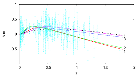
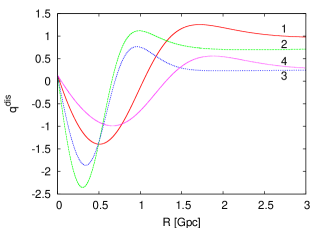
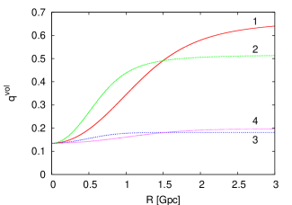
Let us first focus on supernova observations. There is already a considerable literature on inhomogeneous models which are able to fit the supernova observations without the cosmological constant [6]. We shall examine four such models in this section. For each of these models we shall calculate the volume and distance deceleration parameters and compare with each other. The four models to be considered present a very good fit to supernova data. The supernova data consists of 182 supernovae from the Riess gold sample [33]. The $\chi^{2}$ test for models 1-4 is respectively 183.6, 184.3, 164.7, and 178.5 (for comparison the $\chi^{2}$ of fitting the $\Lambda$CDM model is 165.3). The residual Hubble diagram for these models is presented in figure 1. The deceleration parameters for models 1-4 are presented in figure 2. Left panel presents the distance deceleration parameter [as defined by (18) - where $dt/dz$ and $dr/dz$ were calculated for the radial geodesic]. The distance deceleration parameter is positive at the origin, but soon becomes negative. Moreover, a very similar shape is obtained if instead $q^{dis}$ [as defined by (18)] $q^{dis}_{0}$ [as defined by (16)] is used. Thus, $q^{dis}$ (or even $q^{dis}_{0}$, if treated as a function of $r$) can be regarded as a useful test to check if a given model is able to fit supernova data. However, the most significant is that the volume deceleration parameter which is presented in the right panel of figure 2 is strictly positive. Thus, the ability of reproducing the supernova data does not require that the volume deceleration parameter is negative. This raises the question whether the average acceleration has any relation with the observed acceleration of the Universe; and if yes, are models with average acceleration also able to fit supernova data?

Figure 1: The Residual Hubble diagram for models 1-4. The black dashed line presents $\Delta{\rm m}$ for the $\Lambda$CDM model.

Figure 2: The distance deceleration parameter (left panel) and the volume deceleration parameter (right panel) for models 1-4.

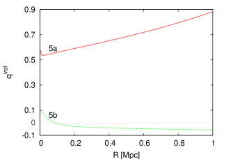
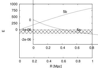
Let us now focus on models of cosmic structures. It was recently shown that using a perturbative approach, backreaction cannot explain the apparent acceleration [34]. However, because of large density fluctuations within cosmic structures, results obtained in terms of the perturbation framework might be questionable. Moreover, in view of the fact that there are known examples of exact inhomogeneous models with negative volume deceleration parameter and $\Lambda=0$, it is worthwhile to check if realistically evolving models of cosmic structures can have negative values of deceleration parameter. First, let us consider a model of galaxy clusters with the Navarro-Frenk-White density distribution [35] (left panel of figure 3). Although, the NFW profile describes virialized systems the use of this profile will prove to be very instructive. The average deceleration parameter $q^{vol}$ for model 5 is presented in the right panel of figure 3. As can be seen in this case the deceleration parameter is positive (curve 5a). However, it is possible to modify this model so that the $q^{vol}$ becomes negative – curve 5b in the right panel of figure 3. This was obtained by choosing the $E$ function which is of large positive value (for details see Appendix). However, after such a modification this model becomes unrealistic. Specifically, the age of the Universe in this model becomes unrealistically small. The bang time function $t_{B}$ in this model is of large amplitude, around $11.44\times 10^{9}$ y. This means that the actual age of the Universe in this model is approximately a few hundreds of thousand years.

Figure 3: The current density distribution (left panel) and deceleration parameter (right panel) for model 5.

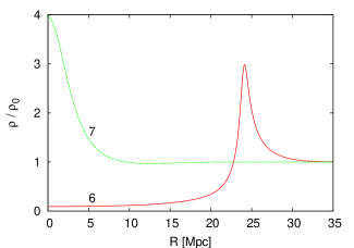
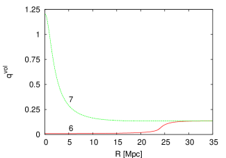
Now let us examine the volume deceleration parameter within models of cosmic voids and superclusters. Figure 4 presents density distribution of realistically evolving cosmic structures (void – curve 6, supercluster – curve 7). It can be seen from the right panel of figure 4 that the volume deceleration parameter within these models is positive. As above, we can modify our models in such a way that the volume deceleration parameter is negative, but again this leads to a very large amplitude of $t_{B}$. For example, in model 8 whose density and the volume deceleration parameter are presented in figure 5 the volume deceleration parameter is negative. However, the bang time function in model 8 is of amplitude $\approx 11\times 10^{9}$ y, which leads to unrealistically small age of the Universe.

Figure 4: The current density distribution (left panel) and volume deceleration parameter (right panel) for models of cosmic structures (models 6, 7).

Figure 5: The current density distribution (left panel) and deceleration parameter (right panel) for model 8.

6 Conclusions

In this paper we have studied the relation between the volume deceleration parameter obtained within the Buchert averaging scheme and the deceleration parameter derived from the observations of supernovae. This work was motivated by recent results showing there there are models which despite $\Lambda=0$ and average expansion rate is accelerating, i.e. $\ddot{a}>0$ [where $a$ is defined by relation (4)]. This opens the possibility that backreaction and averaging effects may be used as an interesting alternative explanation to the dark energy phenomenon.

We have compared the quantities obtained within the exact and inhomogeneous models with their average counterparts. We focused on the supernova observations and models of cosmic structures. For this purpose the Lemaître–Tolman model was employed. It was showed numerically that the averaging of models which fit the supernova observations does not lead to volume acceleration ($\ddot{a}<0$ for these averaged models and hence $q^{vol}>0$). It was also shown that realistically evolving models of cosmic structures have also $q^{vol}>0$. It was possible to modify these model in such a way that after the averaging $q^{vol}<0$. This was obtained by choosing $E$ function of positive amplitude - as was recently proved by Sussman [37] this is a necessary condition to obtain $q^{vol}<0$. However, in models with realistic density distribution, in such a cases, $E\gg 1\gg M/R\approx 10^{-7}-10^{-6}$, hence as seen from (8) $t_{B}\approx t$ (to remind $c\times 10^{10}$y $\approx 3$ Gpc). Thus, within such models the age of the Universe is unrealistically small.

Our analysis has been performed in the limited class of Lemaître–Tolman models, which due to their spherical symmetry are arguably too simple to give a full understanding of averaging and backreaction problems. However, within this class, we conclude that the volume deceleration parameter $q^{vol}$ is not a quantity which can be directly related to observations.

It is possible that the volume deceleration parameter $q^{vol}$ becomes negative only after averaging over the scales which are larger than 100 Mpc. On such large scales the structure of the Universe becomes too complicated to be fully described by spherically symmetric models. However, it is intriguing that models which fit the supernova observations and for which the distance deceleration parameter, $q^{dis}$, is negative have still $q^{vol}>0$. This suggest that the volume deceleration $q^{vol}$ does not have a clear interpretation in terms of observable quantities. It does not, of course, mean that averaging and backreaction effects cannot potentially be employed to explain the phenomenon of dark energy. However, our work here indicates that such a potential solution of the dark energy problem should be based upon different methods than those related to volume deceleration parameter. Rather than showing that $q^{vol}<0$ the averaging approach should explain observations – reproduce correct values of distance to supernovae, correct shape of the CMB power spectrum, etc. An interesting, quasi-Friedmannian approach, was recently suggested in [38]. In this approach backreaction is modeled in terms of the morphon field [28]. In such a case a Universe is describe by a homogeneous model with the spatial curvature being just a function of time. As shown in [38] such approach lead to an agreement with supernova and CMB data without the need for dark energy, but requires $q^{vol}<0$.

Appendix A Model specification

There are three arbitrary functions of the radial coordinate in the Lemaître–Tolman. However only two functions are independent and the third one is specified by the choice of the radial coordinate. Models considered in this paper are defined as follows:

1. Model 1 and 2

   The radial coordinate is chosen as the present day value of the areal distance $r:=R_{0}$. Models 1 and 2 are specified by the present day density distribution and the time bang function. The density distribution is parametrized by

   $$\rho(t_{0},r)=\rho_{b}\left[1+\delta_{\rho}-\delta_{\rho}\exp\left(-\frac{r^{2}}{\sigma^{2}}\right)\right],$$ (19)

   where $\rho_{b}=\Omega_{m}\times(3H_{0}^{2})/(8\pi G)$, $\Omega_{m}=0.27$, $H_{0}=70$ km s^-1 Mpc^-1. In model 1 $\rho_{\delta}=1.9$, $\sigma=0.9$ Mpc, and in model 2 $\rho_{\delta}=1.5$, $\sigma=0.5$ Mpc. In these models the big bang is assumed to occur simultaneously at every point, i.e. $t_{B}=0$. The functions $M$ and $E$ are then calculated and using eqs. (6) and (8) respectively.

   The time instants as well as background density $\rho_{b}$ in all models (1–8) is chosen as density of a Friedmann model ($\Omega_{m}=0.27$, $H_{0}=70$ km s^-1) and time instants are calculated using the following formula [9]:

   $$t(z)=\frac{1}{H_{0}}\int\limits_{z}^{\infty}\frac{d\tilde{z}}{(1+\tilde{z})\sqrt{\Omega_{mat}(1+\tilde{z})^{3}+\Omega_{K}(1+\tilde{z})^{2}}},$$ (20)

   where $\Omega_{K}=1-\Omega_{m}$. The last scattering instant ($t_{LS}$) is set to take place when $z=1089$ and the current instant ($t_{0}$) when $z=0$ — $t_{LS}=4.98\times 10^{5}$ y, and $t_{0}=11.4421\times 10^{9}$ y.

2. Model 3 and 4

   As above the radial coordinate is chosen as the present day value of the areal distance $r:=R_{0}$. These two models are defined by the current expansion rate, and assumption that $\rho(t_{0},r)=\rho_{b}$. The expansion rate is parametrized using

   $$H_{T}(t_{0},r)=\frac{\dot{R}}{R}=H_{0}\left[1-\delta_{H}+\delta_{H}\exp\left(-\frac{r^{2}}{\sigma^{2}}\right)\right],$$ (21)

   where $H_{0}\delta_{H}=9.6$ km s^-1 Mpc^-1, $\sigma=0.6$ Mpc, and $H_{0}\delta_{H}=12$ km s^-1 Mpc^-1, $\sigma=1.2$ Mpc for model 3 and 4 respectively. In these models density is assumed to be homogeneous at the current epoch. The function $M$ is then calculated using the above relation and eq. (7). It should be noted that the $H_{T}$ is one of several generalization of the Hubble constant, which in the Friedmann model is $H_{0}=\dot{a}/a$. Apart from the transverse Hubble parameter, $H_{T}$, one can also define the radial Hubble parameter, $H_{R}$, [see eq. (16)], and the volume Hubble parameter defined as $H_{V}=(1/3)\Theta=H_{R}+2H_{T}$.

3. Model 5a

   The radial coordinate is chosen as the present day value of the areal distance, i.e. $r:=R_{0}$. The model is defined by density distributions given at the present instant and at last scattering. The density distribution at the current instant is parametrized by

   $$\rho(t_{0},r)=\rho_{b}\frac{\delta}{(r/r_{s})(1+r/r_{s})^{2}},$$ (22)

   where $\delta=28170$ and $r_{s}=191kpc$. This is a Navarro, Frenk, and White galaxy cluster profile [35]. As can be seen this profile is singular at the origin but this problem can be overcome by matching the NFW profile with a singular–free profile as $f(r)=-ar^{2}+b$.

   The density profile at last scattering is assumed to be homogeneous, thus the areal distance at last scattering is:

   $$R(t_{LS},r)=\left(\frac{M}{\kappa\rho_{LS}c^{2}}\right)^{1/3}.$$ (23)

   The function $M(r)$ is then calculated from eq. (6). Function $E$ can be calculated by subtracting solutions of (8) for $t_{LS}$ and $t_{0}$ (for details see [39]). The function $E$ is presented in the left panel of figure 6.

4. Model 5b

   The radial coordinate is chosen as the present day value of the areal distance, $r:=R_{0}$. The model is defined by density distribution given by (22) and $E$ of the following form

   $$E(r)=10^{3}\sin\left(10^{-3}r{\rm Mpc}^{-1}\right).$$ (24)

   This profile is presented in the left panel of figure 6 and the bang time function $t_{B}$ in the right panel.

5. Models 6 and 7

   The radial coordinate is chosen as the value of the areal distance at last scattering instant, $r:=R_{LS}$. Model 6 and 7 are defined by the assumption that $t_{B}=0$ and the density distribution, which at last scattering is of the following form

   $$\rho(t_{LS},r)=\rho_{b}\left(1-\delta\exp{(-a\ell^{2}r^{2})}+\gamma\exp{\left[-\left(\frac{\ell r-c}{d}\right)^{2}\right]}\right),$$ (25)

   where $\ell=1/kpc$; $\delta=1.2\times 10^{-3}$ and $2\times 10^{-3}$ for model 6 and 7 respectively; $\gamma=14.62\times 10^{-4}$ and $8.03\times 10^{-4}$ for model 6 and 7 respectively; $a=0.01$ and $0.04$ for model 6 and 7 respectively; $c=18$ and $12$ for model 6 and 7 respectively; and $d=6$ and $5$ for model 6 and 7 respectively. The bang time function for both these models is $t_{B}=0$. The mass function, $M(r)$ is calculated from eq. (6), and the function $E(r)$ is calculated from eq. (8).

6. Model 8

   The radial coordinate is chosen as a present day value of the areal distance: $r:=R_{0}$. Density distribution is of the following form

   $$\rho(t_{0},r)=6.2\rho_{b}\exp{(-4\times 10^{-8}(\ell r)^{2})},$$ (26)

   and the function $E$ is

   $$E(r)=\left(\frac{H_{0}}{c}r\right)^{2}\exp{(10^{-3}\ell r)},$$ (27)

   which except for $[\exp{(10^{-3}\ell r)}]$ is the same as $E(r)$ profile in the empty Universe. This profile is presented in the left panel of figure 7 and the bang time function $t_{B}$ in the right panel.

Figure 6: Left panel presents the function $E(r)$ for models 5a and 5b. Please note that the y-scale in the upper part of the left panel is different than in the lower part. Right panel bang time function for model 5b.

Figure 7: The function $E(r)$ (left panel) and $t_{B}(r)$ (right panel) for model 8.

References

- [1] Perlmutter S et al1997 Astrophys. J. 483 565; Riess A G et al1998 Astrophys. J. 116 1009 Perlmutter S et al1999 Astrophys. J. 517 565
- [2] Hinshaw G et al2008 submitted to Astrophys. J. Suppl. Ser. (Preprint arXiv:0803.0732); Tegmark M et al2006 Phys. Rev. D 74 123507; Percival W J et al2002 Mon. Not. Roy. Astr. Soc. 337 1068
- [3] Ehlers J, Geren P and Sachs R K 1968 J. Math. Phys. 9 1344
- [4] Stoeger W R, Maarteens R and Ellis G F R 1995 Astrophys. J. 443 1
- [5] Nilsson U S, Uggla C, Wainwright J and Lim W C 1999 Astrophys. J. 521 L1
- [6] Dąbrowski M P and Hendry M A 1998 Astrophys. J. 498, 67; Célérier M N 2000 Astron. Astrophys. 353 63; Iguchi H, Nakamura T and Nakao K 2002 Prog. Theor. Phys. 108 809; Godłowski W, Stelmach J and Szydłowski M 2004 Class. Q. Grav. 21 3953; Alnes H and Amarzguioui M 2006 Phys. Rev. D 74 103520; Alnes H. and Amarzguioui M and Grøn Ø 2006 Phys.Rev. D 73 083519; Chung D J H and Romano A E 2006 Phys Rev. D 74 103507; Alnes H and Amarzguioui M 2007 Phys. Rev. D 75 023506; Enqvist K and Mattsson T 2007 J. Cosmol. Astropart. Phys. JCAP07(2007)02019; Alexander S, Biswas T, Notari A and Vaid D 2007 Preprint arXiv:0712.0370; Biswas T, Mansouri R and Notari A 2007 J. Cosmol. Astropart. Phys. JCAP12(2007)017; Brouzakis N, Tetradis N and Tzavara E 2007 J. Cosmol. Astropart. Phys. JCAP0702(2007)013; Brouzakis N, Tetradis N and Tzavara E 2008 J. Cosmol. Astropart. Phys. JCAP0704(2008)008; Marra V, Kolb E W, Matarrese S and Riotto A 2007 Phys. Rev. D 76 123004; Biswas T and Notari A 2008 J. Cosmol. Astropart. Phys. JCAP06(2008)021; Bolejko K 2008 PMC Physics PMCA02(2008)01 (Preprint astro-ph/0512103); García-Bellido J and Haugbøelle T 2008 J. Cosmol. Astropart. Phys. JCAP04(2008)03; Enqvist K 2008 Gen. Rel. Grav. 40 451; Khosravi Sh, Kourkchi E, Mansouri R and Akrami Y 2008 Gen. Rel. Grav. 40 1047; Bolejko K and Wyithe J S B 2008 Preprint arXiv:0807.2891; Yoo C-M, Kai T and Nakao K-i 2008 Preprint arXiv:0807.0932
- [7] Célérier M N 2007 New Adv. Phys. 1 29
- [8] Ellis G F R and Stoeger W 1987 Class. Quant. Grav. 4 1697
- [9] Peebles P J E 1993 Principles of physical cosmology (Princeton: Princeton University Press)
- [10] Ishibashi A and Wald R M 2006 Class. Q. Grav. 23 235
- [11] Kasai M, Asada H and Futamase T 2006 Prog. Theor. Phys. 115 827
- [12] van Elst H and Ellis G F R 1998 Class. Quant. Grav. 15 3545
- [13] Kolb E W, Marra V and Matarrese S 2008 Preprint arXiv:0807.0401
- [14] Ellis G F R 2008 Nature 452 158
- [15] Hellaby C 1988 Gen. Rel. Grav. 20 1203; Lu T H C and Hellaby C 2007 Class. Quant. Grav. 24 4107; McClure M and Hellaby C 2007 Preprint arXiv:0709.0875
- [16] Buchert T 2000 Gen. Rel. Grav. 32 105
- [17] Räsänen S 2006 J. Cosmol. Astropart. Phys. JCAP11(2006)003
- [18] Buchert T 2008 Gen. Rel. Grav. 40 467
- [19] Nambu Y and Tanimoto M 2005 Preprint gr-qc/0507057
- [20] Paranjape A and Singh T P 2006 Class. Quant. Grav. 23 6955
- [21] Kai T, Kozaki H, Nakao K, Nambu Y and Yoo C M 2007 Prog. Theor. Phys. 117 229
- [22] Chuang C H, Gu J A and Hwang W Y P 2008 Class. Quant. Grav. 25 175001
- [23] Räsänen S 2006 Int. J. Mod. Phys. D 15 2141
- [24] Räsänen S 2004 J. Cosmol. Astropart. Phys. JCAP11(2004)010
- [25] Wiltshire D L 2007 New J. Phys. 9 377; Wiltshire D L 2007 Phys. Rev. Lett. 99 251101
- [26] Leith B M, Ng S C C and Wiltshire D L 2008 Astrophys. J. 672 L91
- [27] Khosravi S, Kourkchi E and Mansouri R 2007 Preprint arXiv:0709.2558
- [28] Buchert T, Larena J and Alimi J-M 2006 Class. Q. Grav. 23 6379
- [29] Krasinski A 1997 Gen. Rel. Grav. 29 637; Krasinski A 1997 Gen. Rel. Grav. 29 931; Plebański J and Krasiński A 2006 Introduction to general relativity and cosmology (Cambridge: Cambridge University Press)
- [30] Lemaître G 1933 Ann. Soc. Sci. Bruxelles A 53 51 (1933) (reprinted in 1997 Gen. Rel. Grav. 29 641); Tolman R C 1934 Proc. Nat. Acad. Sci. USA 20 169 (reprinted in 1997 Gen. Rel. Grav. 29 935)
- [31] Hellaby C and Lake K 1985 Astrophys. J. 290 381 (plus errata in 1986 Astrophys. J. 300 461)
- [32] Partovi M H and Mashhoon B 1984 Astrophys. J. 276 4;
- [33] Riess A G et al. 2007 Astrophys. J. 659 98
- [34] Li N, Schwarz D J 2007 Preprint arXiv:0710.5073; Paranjape A and Singh T P 2008 Preprint arXiv:0806.3497
- [35] Navarro J F, Frenk C S and White S D M 1996 Astrophys. J. 462 563
- [36] Hossain G M 2007 Preprint arXiv:0709.3490
- [37] Sussman R A 2008 Preprint arXiv:0807.1145
- [38] Larena J, Alimi J-M, Buchert T, Kunz M and Corasaniti P-S 2008 Preprint arXiv:0808.1161
- [39] Krasiński A and Hellaby C 2002 Phys. Rev. D 65 023501