Microphysical dissipation, turbulence and magnetic fields in hyper-accreting discs

Abstract

Hyper-accreting discs occur in compact-object mergers and in collapsed cores of massive stars. They power the central engine of $\gamma$-ray bursts in most scenarios. We calculate the microphysical dissipation (the viscosity and resistivity) of plasma in these discs, and discuss the implications for their global structure and evolution. At the temperatures ($k_{\rm b}T>m_{\rm e}c^{2}$) and densities ($\rho\sim 10^{9}-10^{12}~{}{\rm gr~{}cm^{-3}}$) characteristic of the neutrino-cooled innermost regions, the viscosity is provided mainly by mildly degenerate electrons, while the resistivity is modified from the Spitzer value due to the effects of both relativity and degeneracy. Under these conditions the magnetic Reynolds number is very large ($R_{\rm eM}\sim 10^{19}$) and the plasma behaves as an almost ideal magneto-hydrodynamic (MHD) fluid. Among the possible non-ideal MHD effects the Hall term is relatively the most important, while the magnetic Prandtl number, $\rm Pm$ (the ratio of viscosity to resistivity), is typically larger than unity: $10\lower 2.15277pt\hbox{$\;\buildrel<\over{\sim}\;$}\rm Pm\lower 2.15277pt\hbox{$\;\buildrel<\over{\sim}\;$}6\times 10^{3}$. Inspection of the outer radiatively inefficient regions indicates similar properties, with magnetic Prandtl numbers as high as $\sim 10^{4}$. Numerical simulations of the magneto-rotational instability (MRI) indicate that the saturation level and angular momentum transport efficiency may be greatly enhanced at high Prandtl numbers. If this behaviour persists in the presence of a strong Hall effect we would expect that hyper-accreting discs should be strongly magnetised and highly variable. The expulsion of magnetic field that cannot be dissipated at small scales may also favour a magnetic outflow. We note that there are limited similaries between hyper-accreting discs and X-ray binary discs – which also have a high magnetic Prandtl number close to the black hole – which suggests that a comparison between late-time activity in $\gamma$-ray bursts and X-ray binary accretion states may be fruitful. More generally, our results imply that the possibly different character of high Prandtl number MHD flows needs to be considered in studies and numerical simulations of hyper-accreting discs.

1 Introduction

The fluid dynamics of dense accretion discs is described by the Navier-Stokes and magneto-hydrodynamic equations. Within such a description, the microscopic properties of the fluid are parameterized (in part) via the kinematic viscosity $\nu$, which describes the rate at which inter-particle collisions damp fluid motions, and the resistivity $\eta$, which quantifies the dissipation of currents via Ohmic losses. Timescales can be associated with each of these quantities. The viscous timescale of a disc $t_{\rm acc}=r^{2}/\nu$, for example, is the timescale on which the microscopic viscosity would lead to angular momentum transport over a scale $r$. As is well known (Pringle, 1981), for astrophysical discs the timescales for evolution driven by the microscopic viscosity are many orders of magnitude larger than the observed evolution timescales. It is therefore generally assumed that evolution is driven by an “anomalous” or “turbulent” viscosity $\nu_{\rm t}\gg\nu$ (Shakura & Sunyaev, 1973), possibly augmented in some cases by angular momentum loss in a wind (Blandford & Payne, 1982). In most astrophysical discs $\nu_{t}$ is likely generated from turbulence driven by the magneto-rotational instability (MRI; see Balbus & Hawley (1998) and references therein). Since $\nu_{\rm t}\gg\nu$ most studies of discs make the implicit assumption that the actual values of $\nu$ and $\eta$ are unimportant, and consider instead evolution under the action of the effective transport coefficients $\nu_{t}$ and $\eta_{t}$.

Provided that the Reynolds ($R_{\rm e}$) and magnetic Reynolds ($R_{\rm eM}$) numbers are large enough, the absolute value of either one may indeed be of little import for accretion discs. Their ratio, however, which we define as the magnetic Prandtl number,

$${\rm Pm}\equiv\frac{\nu}{\eta}$$ (1)

is almost certainly not ignorable (Balbus & Hawley, 1998). An accretion disc serves to convert the large-scale energy present in the shear flow into other energy forms – turbulent kinetic energy, magnetic field, and heat – and the dissipation required to generate heat may vary strongly depending upon the microphysical transport coefficients. In particular, if ${\rm Pm}\gg 1$ the plasma is highly viscous on the scale at which resistivity operates. In this regime one may expect that dissipation of the magnetic field will be suppressed, with a resulting modification in the saturation level of dynamo generated fields and an inverse cascade of magnetic energy to large scales (Brandenburg, 2001). The importance of the magnetic Prandtl number for the resulting magnetic field structure has been illustarted analytically (Umurhan, Menou & Regev, 2007a; Umurhan, Regev & Menou, 2007b) and numerically, both in idealised simulations of dynamo action within forced turbulence (Schekochihin et al., 2004) and in local shearing-box simulations of the MRI within accretion discs (Lesur & Longaretti, 2007; Fromang et al., 2007). For discs the current limited set of simulations indicates that the efficiency of angular momentum transport, parameterized via the Shakura-Sunyaev $\alpha$ parameter, increases with ${\rm Pm}$, and can approach $\alpha\sim 1$ given the combination of modest ${\rm Pm}=8$ and a weak net vertical magnetic field. Motivated by these results, Balbus & Henri (2008) calculated the expected radial variation of ${\rm Pm}$ within standard Shakura-Sunyaev models of geometrically thin, radiatively efficient accretion discs. They found that ${\rm Pm}$ exceeds unity within $\sim 50$ Schwarzschild radii of the central object, and suggested that the qualitatively different behaviour of the MRI in the high ${\rm Pm}$ limit might be responsible for the time-dependent outbursts and state changes that are observed in X-ray binaries.

In this paper, we compute the magnitude and radial dependence of the magnetic Prandtl number in hyper-accreting discs. Such discs, which can support accretion rates of the order of $1\ M_{\odot}\ {\rm s}^{-1}$, form from compact object mergers (e.g. Ruffert & Janka, 1999) and when the cores of rapidly rotating massive stars collapse (Woosley, 1993). The disc structure is shaped by neutrino emission in the regions close to the accreting object, while in the outer parts neither neutrinos (the temperature is too low) nor photons (which are trapped within the flow) can provide cooling. Hyper-accreting discs are invoked to provide the initial energy injection in many models for $\gamma$-ray bursts (GRBs). Our ultimate motivation for studying the magnetic Prandtl number in these discs is to understand the complex phenomenology (jets, highly variable prompt emission, X-ray flares, plateau phases etc) that is observed in GRBs (e.g. Burrows et al., 2005) and which may well derive from the evolution of the disc.

We anticipate different results from those found by Balbus & Henri (2008) for photon-cooled discs. In the neutrino-cooled region the differences arise from two reasons. First, since neutrino opacities are vastly smaller than photon opacities, hyper-accreting discs are much cooler and denser than an extrapolation of Shakura-Sunyaev discs would imply, and this on its own would alter the magnetic Prandtl number. Second, the temperatures and densities in hyper-accreting discs are such that the electrons are mildly relativistic and mildly degenerate, while the elastic collision cross-section for the nuclei exceeds the Coulomb cross-section. As a consequence, the classical Spitzer (1962) expressions for $\nu$ and $\eta$, which are adequate for ordinary accretion flows, no longer apply. They do apply, instead, in the outer regions of hyper-accreting discs, where a different $\rm Pm$ behaviour occurs since the flow is radiatively inefficient and photon-pressure dominated.

The organization of this paper is as follows. In §2 through §5 we describe the formalism for calculating the structure of hyper-accreting discs. This is required here in order to determine consistently the plasma conditions within these discs – including the temperature, density, nuclear composition and degree of degeneracy. Readers familiar with vertically averaged hyper-accreting disc models will find that our approach generally follows standard practice. The structure of the resulting disc models is presented in §6. Given these conditions, we then calculate in §7 and §8 the resisitivity and viscosity in the neutrino cooled inner region of the disc. These Sections contain the principle new results of this paper. Combining the viscosity and resistivity, we show in §10 that ${\rm Pm}>1~{}{\rm or}\gg 1$ across the entire radial range relevant for GRB models. In §11 we estimate the strength of other non-ideal MHD effects, and in §12 we study the structure of the outer non-radiative region of the disc. §13 and §14 discuss and summarize our results, and what they may imply for disc evolution and GRB observables.

2 The disc model

We calculate the temperature and density at the midplane of a hyper-accreting disc from vertically averaged thin disc solutions. In hyper-accreting discs the diffusion time for photons to leak out from the disc is much larger than the accretion time scale ($t_{\rm diff}/t_{\rm acc}\sim 10^{11}$) and photons remain trapped. However, for sufficiently high accretion rates the temperature in the innermost region exceeds $\sim$ 1 MeV and neutrino production switches on (Popham, Woosley & Fryer 1999). This happens for radii r $\lower 2.15277pt\hbox{$\;\buildrel<\over{\sim}\;$}100~{}r_{\rm S}$, where $r_{\rm S}=2\,GM_{\rm BH}/c^{2}$ is the Schwarzschild radius for a black hole of mass $M_{\rm BH}$. The neutrino flux liberates the energy deposited locally by viscous (turbulent) stresses and consequently the local sound speed $c_{\rm s}$ remains smaller than the rotational velocity ($v_{\phi}$) of the disc. Such discs are geometrically thin (the vertical scale height is small compared to the radius), and can be described by a modified version of the standard “$\alpha-$disc” theory (Shakura & Sunyaev 1973). Many previous studies of hyper-accreting discs have adopted this formalism (e.g. Popham, Woosley & Fryer, 1999; Narayan, Piran & Kumar, 2001; Kohri & Mineshige, 2002; Di Matteo, Perna & Narayan, 2002; Chen & Beloborodov, 2007, and references therein). In what follows we consider only the innermost region ($r\leq 70~{}r_{\rm S}$) where neutrino cooling is generally efficient. For simplicity the accretion rate is assumed to be time-independent, but our basic results for the magnetic Prandtl number would carry over locally to real discs in which the accretion rate varies with radius and time.

In a steady state, conservation of mass and angular momentum for a differentially rotating fluid yield a relation between the surface density $\Sigma$ and the radial mass flow $\dot{M}$,

$$\Sigma\,\nu_{\rm t}=\frac{\dot{M}}{3\,\pi}\,\left[1-\left(\frac{r_{*}}{r}\right)^{1/2}\right],$$ (2)

where the fluid equations have been averaged in the vertical ($\vec{z}$) direction over the pressure scale height $H=-P/(dP/dz)$. We assume that no viscous torque is acting at the location of the innermost stable orbit $r_{*}=3~{}r_{\rm S}$. Consistent with the thin disc approximation radial pressure gradients have been neglected and the orbital velocity is simply $v_{\phi}^{2}=GM_{BH}/r$ (the “Keplerian velocity”). The surface density is related to the midplane ($z=0$) density via $\Sigma=\rho H$. The radial mass flow $\dot{M}$ [gr s^-1] is defined by the continuity equation

$$\dot{M}=-2\pi r\Sigma v_{\rm r}={\rm constant},$$ (3)

where the radial drift velocity $v_{\rm r}$ is subsonic. The turbulent kinematic viscosity is parameterized as (Shakura & Sunyaev, 1973; Lynden-Bell & Pringle, 1974) ,

$$\nu_{\rm t}=\alpha\,c_{\rm s}\,H.$$ (4)

We emphasise here that the kinematic viscosity $\nu_{\rm t}$ is quite different in nature from the “microscopic” (also referred to as “molecular”) viscosity $\nu$, that enters into the definition of the magnetic Prandtl number. The first is associated with turbulent flow and magnetic stresses in the plasma, while the second is given by deflection of ions and electrons by particle-particle collisions in the plasma.

For a thin disk both radial advection of energy and flux in the radial direction can typically be neglected (we justify this for our case later). From energy conservation the heating dissipated locally by viscous stresses is emitted per unit area through the surface of the disc as neutrino $F_{\nu}$ and anti-neutrino flux $F_{\bar{\nu}}$ :

$$\frac{9}{8}\,\nu\,\Sigma\,\Omega^{2}=F_{\nu}+F_{\bar{\nu}}.$$ (5)

The calculation of the flux in the optically thin and optically thick regions of the disc is detailed in the next section. Eq. 2 and eq. 5 allow us to solve for the disc structure once the equation of state is specified. In the inner regions that we are considering, densities ($\rho\sim 10^{8}-10^{11}$ gr cm^-3) are high for the temperatures of interest ($T\simeq$ a few $10^{10}$ K). This has a number of consequences. First, electrons are mildly degenerate ${\mu}/{\theta}\sim{\rm a~{}few}$, where $\mu$ is the chemical potential in units of the electron rest mass energy $m_{\rm e}c^{2}$ and $\theta={k_{\rm b}T}/({m_{\rm e}c^{2}})$, where $k_{\rm b}$ is the Boltzmann constant. Second, the plasma is neutron rich. If $Y_{\rm p}$ is the number fraction of protons over baryons, $Y_{\rm p}\sim 0.1$. Finally, the baryon pressure

$$P_{\rm b}=\frac{\rho}{m_{\rm p}}\,k_{\rm b}T,$$ (6)

dominates the total pressure $P$ (e.g. Beloborodov, 2003), and the isothermal sound speed $c_{s}^{2}=P/\rho$ is,

$$c_{\rm s}=1.6\times 10^{9}\left(\frac{T}{3\times 10^{10}}\right)^{1/2}{\rm cm/s}.$$ (7)

At larger radii, on the other hand, the density is smaller, ${\mu}/{\theta}\lower 2.15277pt\hbox{$\;\buildrel<\over{\sim}\;$}1$, and electron and photon pressure are more important (e.g. Narayan, Piran & Kumar, 2001). Note that in eq. 6, and henceforth, we ignore the mass difference between protons and neutrons. We also assume that all the baryons are free, since $\alpha$ particles present at larger radii have been photo-dissociated. This is a valid approximation since, for the parameters we use in our disc structure models, $\alpha$ particles do not constitute more than 10% of the baryons (see e.g. Chen & Beloborodov, 2007, thereafter CB07).

The neglect of advection in eq. 5 is generally a good approximation. The ratio of neutrino diffusion time to accretion time is

$$\frac{t_{\rm diff,\nu}}{t_{\rm acc}} = \frac{\tau_{\nu}H}{c}\,\frac{\nu_{\rm t}}{r^{2}}$$ (8)

$$\simeq 6\times 10^{-4}\tau_{\nu}\left(\frac{\alpha}{0.1}\right)\left(\frac{H/r}{0.3}\right)^{3}\left(\frac{r/r_{\rm S}}{10}\right)^{-1/2}$$

and hence advection is important only if the optical depth to neutrinos is of the order of $10^{3}$ or higher. In our models optical depths are, at most, $\tau_{\nu}\sim$ a few tens, unless the accretion rate is very large, (e.g. $\dot{M}\lower 2.15277pt\hbox{$\;\buildrel>\over{\sim}\;$}10~{}M_{\sun}$sec^-1, for $\alpha=0.1$). For a maximally rotating Kerr black hole (not treated here), advection can become important for lower accretion rates: $\dot{M}\lower 2.15277pt\hbox{$\;\buildrel>\over{\sim}\;$}2~{}M_{\sun}$sec^-1, for $\alpha=0.1$ (CB07). Advection of energy in photons instead can play a role in the region we consider for $\alpha\lower 2.15277pt\hbox{$\;\buildrel>\over{\sim}\;$}0.1$, since the outer radiatively inefficient part of the disc can extend inward, within $70~{}r_{\rm S}$. We will comment on this in § 6.

3 The neutrino flux

At the temperatures and densities of interest for the inner regions of hyper-accreting discs neutrinos are produced primarily by electron capture onto protons

$$p+e^{-}\rightarrow n+\nu$$ (9)

while anti-neutrinos are produced by positron capture onto neutrons

$$n+e^{+}\rightarrow p+\bar{\nu}.$$ (10)

The inverse of these processes – namely neutrino absorption by nuclei – constitute one source of neutrino opacity, others (discussed in § 5) are neutrino scattering by both nuclei and electrons. We note that at threshold reaction 9 can proceed if the electron has an energy equal to the mass difference between a neutron and a proton. In this case the emitted neutrino has zero energy. The mild degeneracy of electrons suppresses the pair annihilation channel $e^{+}+e^{-}\rightarrow\nu+\bar{\nu}$, since positrons are exponentially reduced with respect to electrons:

$$\frac{n_{+}}{n_{-}}\propto\exp{\left[-\frac{2\mu}{\theta}\right]}\ll 1.$$ (11)

At equilibrium and neglecting advection, the capture rates  9 and 10 should be equal (see also § 4). We therefore set $F_{\nu}=F_{\bar{\nu}}$ and derive only the neutrino flux. The calculation basically follows the CB07 prescription.

For $e^{-}$ capture onto protons (9), the emissivity in units of $m_{\rm e}c^{2}$ is,

$$\epsilon_{\nu}=k\rho_{\rm p}\int_{Q}^{\infty}(e-Q)^{3}F(e,\mu_{-})e^{2}\sqrt{1-\frac{1}{e^{2}}}\,de,$$ (12)

(e.g. Shapiro & Teukolsky 1983), where $e$ is the electron energy in units of $m_{\rm e}c^{2}$, $Q={(m_{n}-m_{p})}/{m_{e}}$, the matter density of protons is defined as $\rho_{\rm p}=Y_{\rm p}\rho$, and $k=6.5\times 10^{-4}$ is a constant. The function $F(e,\mu)$ is the Fermi-Dirac distribution,

$$F(e,\mu)=\frac{1}{\exp[{\left(\frac{e-\mu}{\theta}\right)}]+1}.$$ (13)

The energy density in units of $m_{\rm e}c^{2}$ for an optically thin disc can be expressed in terms of the emissivity as

$$U_{\nu,n}=\epsilon_{\nu}\frac{H}{c}.$$ (14)

If, conversely, the optical depth $\tau_{\nu}\gg 1$, neutrinos thermalize to a Fermi-Dirac distribution (eq. 13) and the energy density in units of $m_{\rm e}c^{2}$ is given by,

$$U_{\nu,c}=\frac{(m_{\rm e}\,c)^{3}}{2\pi^{2}\hbar^{3}}\int_{o}^{\infty}F(e_{\nu},\mu_{\nu})\,e_{\nu}^{3}\,de_{\nu}.$$ (15)

For $\mu_{\nu}=0$, $U_{\nu,c}=24.5\,k_{\rm b}T^{4}$. To deal with regions of the disc that have $\tau_{\nu}\sim 1$ we interpolate between the optically thin and thick limits. We define

$$x=\frac{U_{\nu,n}}{U_{\nu,n}+U_{\nu,c}}$$ (16)

and express the neutrino flux for arbitrary optical thickness as

$$\frac{F_{\nu}}{m_{\rm e}c^{2}}=\left\{\begin{array}[]{ll}U_{\nu,n}\,c(1+\tau_{\nu})^{-1}&\mbox{for $x<\frac{1}{2}$},\\ U_{\nu,c}\,c\,(1+\tau_{\nu})^{-1}&\mbox{for $x\geq\frac{1}{2}$}.\end{array}\right.$$ (17)

4 Nuclear composition

In the mid-plane of the disc pairs, baryons (free protons and neutrons only in our case) and photons are in thermodynamic equilibrium. For given ($\rho$, $T$), and specified optical depth, this fact suffices to determine the nuclear composition of the plasma. In practice we compute the composition in the optically thick and optically thin limits separately, and deal with the intermediate regime by making an interpolation that is consistent with charge conservation.

Let us first note some general considerations. In addition to the processes of electron / positron capture onto nuclei (equations 9 and 10), pairs are created and absorbed via

$$e^{+}+e^{-}\leftrightarrow\gamma+\gamma.$$ (18)

This implies that

$$\mu=\mu_{-}=-\mu_{+}.$$ (19)

Baryons, instead, are created and destroyed only according to the processes given by equations 9 and 10. Therefore, at equilibrium (${dY_{\rm p}}/{dt}=0$), and neglecting advection, the emissivity for neutrinos and anti-neutrinos must everywhere be equal.

In regions of the disc that are very optically thick to neutrinos, they will have relaxed into a Fermi-Dirac distribution and the above condition can be expressed as,

$$n_{\nu}=n_{\bar{\nu}},$$ (20)

where the number densities are calculated by integrating eq. 13 over momenta with the statistical weight set to unity. The equality of the neutrino and anti-neutrino number densities (eq. 20) implies a vanishing neutrino chemical potential,

$$\mu_{\nu}=\mu_{\bar{\nu}}=0.$$ (21)

The chemical balance of reactions 9 and 10 (and their inverses) $\mu_{\rm p}+\mu=\mu_{n}+\mu_{\nu}$ gives

$$\mu=\theta\ln{\frac{n_{\rm n}}{n_{\rm p}}}+Q,$$ (22)

(Beloborodov, 2003) where protons and neutrons (with number density $n_{\rm p}$, $n_{\rm n}$ respectively) have a Maxwellian distribution.

For regions of the disk that are optically thin, we use

$$\dot{n}_{\nu}=\dot{n}_{\bar{\nu}},$$ (23)

where the number of neutrinos $\nu$ and anti-neutrinos $\bar{\nu}$ emitted per unit volume per unit time is

$$\dot{n}_{\nu}=k\rho_{\rm p}\int_{Q}^{\infty}(e-Q)^{2}F(e,\mu_{-})\,e^{2}\sqrt{1-\frac{1}{e^{2}}}\,de,$$ (24)

and

$$\dot{n}_{\bar{\nu}}=k\rho_{\rm n}\int_{1}^{\infty}(e+Q)^{2}F(e,\mu_{+})\,e^{2}\sqrt{1-\frac{1}{e^{2}}}\,de,$$ (25)

(e.g. Shapiro & Teukolsky 1983).

In both regimes, we impose the conditions of charge neutrality,

$$n_{-}+n_{+}=Y_{p}\frac{\rho}{m_{p}},$$ (26)

where

$$Y_{p}=\frac{n_{p}}{n_{b}},$$ (27)

and baryon conservation,

$$1-\frac{n_{n}}{n_{p}+n_{n}}=Y_{\rm p}.$$ (28)

The electron $n_{-}$ and positron $n_{+}$ number densities are obtained by directly integrating eq. 13 over momenta with the statistical weight set to two. To summarise, we use two different sets of equations in the two extreme regimes: when $\tau_{\nu}\gg 1$, we find $Y_{\rm p}=Y_{\rm p,c}$ and $\mu=\mu_{\rm c}$ from eqs. 22, 26 and 28; when $\tau_{\nu}\ll 1$, we find $Y_{\rm p}=Y_{\rm p,n}$ and $\mu=\mu_{\rm n}$ from eqs. 23, 26 and 28.

Matter in the disc plane, of course, can have an arbitrary optically thickness. To compute the nuclear composition for specified $\rho$ and $T$ we first interpolate to find the chemical potential using,

$$\mu=(1-x)\mu_{\rm n}+x\mu_{\rm c},$$ (29)

where $x$ is given by eq. 16. We then find the proton fraction $Y_{\rm p}$ by imposing charge conservation (eq. 26). The resulting $Y_{\rm p}$ is $Y_{\rm p,n}\leq Y_{\rm p}\leq Y_{\rm p,c}$.

Physically, the most important trends in the nuclear composition can be understood in terms of the ratio of the temperature to the (relativistic) degeneracy temperature

$$T_{\rm deg}\simeq 0.71\left(\frac{\rho Y_{\rm p}}{m_{\rm p}}\right)^{1/3}\rm K,$$ (30)

where we set $n_{\rm p}=n_{\rm-}=\rho Y_{\rm p}/m_{\rm p}$. If $T<T_{\rm deg}$ (at low temperature, or at high density) then $\mu$ increases, positrons are suppressed (eq. 11), and the resulting plasma is neutron-rich (low $Y_{\rm p}$). In the opposite limit of $T\gg T_{\rm deg}$, $n_{+}\simeq n_{-}$ but $Y_{\rm p}\lower 2.15277pt\hbox{$\;\buildrel>\over{\sim}\;$}0.5$ because, as noted before, reaction 10 is energetically favoured.

5 Opacities

The vertical optical thickness of the disk to $\nu$ and $\bar{\nu}$ in eq. 17

$$\tau_{\nu}=H\rho\kappa,$$ (31)

is calculated considering three sources of opacity: $\kappa=\kappa_{\rm a}+\kappa_{\rm s,e}+\kappa_{\rm s,b}$ [cm² gr^-1]. First, absorption onto nuclei,

$$\kappa_{\rm a}=\frac{0.5}{m_{\rm p}}\left(\sigma_{\nu,\rm n}(1-Y_{\rm p})+\sigma_{\bar{\nu},\rm p}Y_{\rm p}\right)$$ (32)

where $\sigma_{\nu,\rm n(p)}$ is the cross section for $\nu$ ($\bar{\nu}$) absorption by neutrons (protons). Second, elastic scattering by electrons,

$$\kappa_{\rm s,e}=0.5\frac{Y_{\rm e}}{m_{\rm p}}\left(\sigma_{\rm e,\nu}+\sigma_{\rm e,\bar{\nu}}\right),$$ (33)

where $Y_{\rm e}={n_{-}}/{n_{\rm b}}$ and $\sigma_{\rm e,\nu(\bar{\nu})}$ is the electron-neutrino (anti-neutrino) cross section. We neglect scattering onto positrons since $n_{+}/n_{-}\ll 1$. Finally, elastic scattering by nuclei,

$$\kappa_{\rm s}=\left(0.3~{}Y_{\rm p}+0.36~{}(1-Y_{\rm p})\right)\frac{\sigma_{0}}{m_{\rm p}}\,\bar{E}_{\nu}^{2},$$ (34)

where $\sigma_{0}=1.7\times 10^{-44}$ cm². For the explicit forms of the cross sections, we refer the reader to the Appendix B of CB07.

The cross sections for these processes depend on the neutrino energy, and the total cross section $\sigma$ should be derived by integrating over the neutrino spectrum. This requires knowledge of the neutrino distribution function at arbitrary optical depth. We, instead, use approximate mean cross sections, which are adequate for our purposes. We first evaluate $\sigma$ at a mean neutrino energy (in unit of $m_{\rm e}c^{2}$) :

$$\sigma=\sigma(\bar{E}_{\nu}).$$

Then, the usual interpolation allows us to link the optically thin and thick regimes:

$$\bar{E}_{\nu}=(1-x)\,\bar{E}_{\nu,\rm n}+x\,\bar{E}_{\nu,\rm c},$$ (35)

(CB07) where

$$\bar{E}_{\nu,\rm n}=\frac{\epsilon_{\nu}}{\dot{n}_{\nu}},$$ (36)

corresponding to $\tau_{\nu}\ll 1$ and

$$\bar{E}_{\nu,\rm c}\simeq 3.17\;\frac{k_{\rm b}T}{m_{\rm e}c^{2}},$$ (37)

corresponding to $\tau_{\nu}\gg 1$ is the mean energy calculated from a Fermi-Dirac distribution function with zero chemical potential. We use the same treatment for anti-neutrino cross sections.

In practice, we find that for conditions appropriate to our disc models absorption by nuclei is always the dominant opacity by one or two orders of magnitude. Electron scattering is least important.

6 Results for the disc structure

Figure 1: Midplane temperature as a function of radius (in units of the Schwarzschild radius $r_{\rm S}$), for three disc models computed for $M_{\rm BH}=3\,M_{\sun}$ and $\alpha=0.1$. The accretion rates are indicated in the legend.

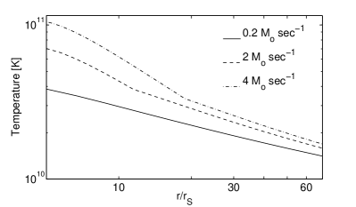
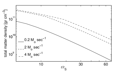
To give an idea of the midplane temperatures and densities encountered in hyper-accreting discs, we show in Figure 1 and Figure 2 illustrative examples of the radial profiles of these quantities. The disc models plotted were computed for a black hole of $3~{}$M_☉, with $\alpha=0.1$ and accretion rates of $0.2$, $2$ and $4~{}$M_☉sec^-1. For these parameters the disc is optically thin across the entire radial range shown for the lowest value of the accretion rate. For the two high accretion rate models the disc is optically thick within about $15r_{\rm S}$ of the black hole.

The most important feature of the neutrino cooled solutions for our purposes is the relatively weak radial dependence of the temperature. As noted elsewhere (e.g. CB07), the disc self-adjusts to maintain electrons in a state of mild degeneracy (i.e. $T\approx 0.3-0.5T_{\rm deg}$): higher degeneracy would cause the cooling to decrease drastically and the temperature to rise, lifting the degeneracy, and vice versa for lower degeneracy. This thermostatic aspect of neutrino cooled discs has as a consequence that temperature does not vary strongly with radius, since the degeneracy temperature depends only weakly on density (and in addition $Y_{\rm p}$ decreases with $\rho$). The proton fraction $Y_{\rm p}$ is everywhere less than $0.3$, falling to around $Y_{\rm p}\sim 0.1$ in the innermost regions.

We have verified that the physical conditions in our disc models reproduce those of prior authors. Comparing our results to those of CB07, we find excellent agreement – especially for $\alpha<0.1$ – between our models with a given $\alpha$ and their model with $\alpha/2$ (the factor two arises primarily due to different definitions of viscosity and different inner boundary conditions, both of which are largely arbitrary). For $\alpha=0.1$, their densities are lower and the advection dominated outer region (which is not cooled efficiently by neutrinos) extends to smaller radii. Since we ignore the advective term in the energy equation, our profiles have a different slope but they never differ by more than a factor of 2 in density and by 50% in temperature.

Figure 2: The same as fig. 1 but for the midplane total matter density.

7 Electrical resistivity of the plasma

The computation of the resistivity of a plasma in which electrons are both relativistic and degenerate is quite subtle, and ultimately requires numerical methods. We first review some general considerations, including the classical Spitzer (1962) result, which we emphasise is not applicable to hyper-accreting discs. These results will prove useful later when we discuss the relative importance of different non-ideal MHD effects.

7.1 General considerations

The electrical resistivity of a plasma is a measure of the electron mobility in the presence of an applied electric field. Acceleration due to the electric field ($e\vec{E}$, where $e$ is now the electric charge) is opposed by drag from (primarily) electron-proton collisions. Balancing these competing forces on a electron of velocity $v$ and momentum $p=\gamma_{\rm e}\,m_{\rm e}v$,

$$e\vec{E}=\frac{p}{t_{\rm ep}},$$

where we neglect pressure gradients and magnetic fields and assume stationary protons. Ohm’s law then gives,

$$\eta=\frac{\gamma_{\rm e}}{4\pi r_{\rm e}n_{-}t_{\rm ep}},$$ (38)

(see e.g. Jackson 1963 p. 460, for the non-relativistic derivation). In this expression $n_{-}$ is strictly equal to $n_{-}(p)$: the number density of electrons with momentum $p$, $\gamma_{\rm e}$ is the electron Lorentz factor, $r_{\rm e}=e^{2}/m_{\rm e}c^{2}\simeq 2.82\times 10^{-13}{\rm cm}$ is the classical electron radius and $t_{\rm ep}$ is the proton-electron deflection time. The associated electrical conductivity is $\sigma=c^{2}/(\eta 4\pi)$. Extending the non-relativistic definition (that can be found for example in Longair 1992, p. 304), $t_{\rm ep}$ can be defined so that $\left<\Delta p_{\perp}^{2}\right>\,t_{ep}=p^{2}$, where $\left<\Delta p_{\perp}^{2}\right>$ is the mean square impulse received by an electron per scattering perpendicular to its direction of motion. We obtain

$$t_{\rm ep}=\frac{p^{2}\,v}{8\pi n_{\rm p}e^{4}\log\Lambda_{\rm ep}(p)},$$ (39)

where $\log\Lambda_{\rm ep}(p)$ is the Coulomb logarithm, defined as the logarithm of the maximum to the minimum impact parameter for proton-electron collisions.

If we take the non-relativistic limit ($\gamma_{\rm e}\rightarrow 1$) of eqs. 38  and  39 and insert the mean thermal velocity of non-degenerate electrons $v=\bar{v}_{\rm e}=\sqrt{{8k_{\rm b}T}/\pi{m_{\rm e}}}$, we recover the scalings derived by Spitzer (1962) for a completely ionized plasma with $n_{\rm p}=n_{-}$

$$\eta_{\rm S}=1.9\times 10^{12}\log\Lambda_{\rm ep,S}\,T^{-3/2}\;{\rm\frac{cm^{2}}{sec}},$$ (40)

where the Coulomb logarithm for electron-proton collision is:

$$\Lambda_{\rm ep,S}=1.24\times 10^{4}\frac{T^{3/2}}{\sqrt{n_{-}}}\sqrt{\frac{4.2\times 10^{5}}{T}}.$$ (41)

In this non-degenerate regime, the (inverse) dependency of $\eta_{\rm S}$ on density is weak.

7.2 Numerical computation of $\eta$

To compute the plasma resistivity under our conditions of temperature and density, we use the code by Potekhin (1999) and Potekhin et al. (1999), which is able to treat arbitrary degeneracy of fully relativistic electrons (but not positrons). The calculation involves an integration of eq. 38 over energy, weighted by the Fermi-Dirac distribution (eq. 13). The Coulomb logarithm is calculated via an effective scattering potential that takes into account Debye charge screening (see reference above for details). We use as input parameters to the code the temperature $T$ and the proton density $\rho_{\rm p}$, which, in turn, depends (via $Y_{\rm p}$) on $T$ and $\rho$. From $\rho_{\rm p}$ the code derives the electron density and thus the electron chemical potential which uniquely specifies the electron Fermi-Dirac distribution.

In principle the calculation of the total resistivity should include the contribution of positrons both as charge carriers (they contribute to the current density and have their own resistivity) and as deflectors for electrons. However, we have already noted that positrons are exponentially suppressed with respect to electrons and from charge conservation it follows that they can also be neglected in the drag force which remains dominated by protons.

The code allow us to explore the plasma resistivity under different condition of electron degeneracy. In the non-degenerate limit the resistivity decreases with temperature, because scattering becomes less frequent, while the density dependence is weak and confined to the Coulomb logarithm (e.g. Spitzer resistivity, eq. 40, for $k_{\rm b}T\ll m_{\rm e}c^{2}$). In the highly-degenerate regime, instead, the resistivity increases with temperature, because more energy states become available for the electrons to be scattered into. The density dependence here is strong. Higher density (for fixed temperature) results in higher degeneracy and suppression of scattering: the plasma resistivity thus decreases. The intermediate mildly degenerate regime, where the resistivity changes very slowly with temperature and density, is the one occupied by our plasma.

7.3 Results

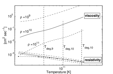
The calculated resistivity is shown as a function of temperature in Figure 3. For a density of $\rho=10^{10}\ {\rm gr}\ {\rm cm}^{-3}$ the degeneracy temperature $T_{\rm deg,10}$ (evaluated at $\rho_{\rm p}=0.5\times 10^{10}\ {\rm gr}\ {\rm cm}^{-3}$) is approximately $10^{11}$ K. For temperatures above this value, the proton fraction remains approximately constant at a value of $Y_{\rm p}\simeq 0.5$, thus $\rho_{\rm p}$ does not change appreciably and the resistivity decreases with temperature since electron-proton collisions becomes less frequent. For lower temperatures, one’s naive expectation is that the resistivity ought to flatten out and eventually decrease as electrons become more and more degenerate. This behaviour is seen if we artificially impose a temperature independent electron density (dashed line), but it does not reflect the physical behaviour of the disc plasma. In fact, as the temperature drops toward and below $T_{\rm deg,10}$ the plasma becomes more and more neutron-rich (i.e. $Y_{\rm p}$ decreases), with an attendant decrease in the electron density. The effective degeneracy temperature decreases, and the electrons never become highly degenerate. The overall result is that at “low” temperatures the electrons self-adjust toward a mildly degenerate regime in which $\eta$ rises slowly with decreasing temperature. The dependence on density is weak.

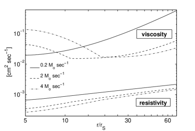
Within a hyper-accreting disc, the midplane temperature is a fairly weak function of radius (Figure 1). This, when coupled with the weak dependence of the resistivity on density, results in a radial profile of $\eta$, shown in Figure 4, that increases slowly with distance from the black hole. Between 5 and $70~{}r_{\rm S}$ the variation in the resistivity is less than an order of magnitude. There is a modest decrease with increasing accretion rate.

Figure 3: The microscopic viscosity (upper curves) and electrical resistivity (lower curves) as a function of temperature, for three different densities: $\rho=10^{9}$ gr cm^-3 (dot-dashed line), $\rho=10^{10}$ gr cm^-3 (solid line) and $\rho=10^{11}$ gr cm^-3 (dashed line). These curves are calculated with a self-consistent nuclear composition and chemical potential $\mu$. The resistivity curve plotted with a dashed line with dots is computed for $\rho=10^{10}$ but with a fixed nuclear composition, $Y_{\rm p}\simeq 0.5$, and the corresponding $\mu$ for each temperature: this forces the electrons to become degenerate as $T$ decreases. The proton fraction $Y_{\rm p}\simeq 0.5$ corresponds to the maximum temperature ($\sim 2\times 10^{11}$ K) considered here, for any shown density. All curves are computed in the optically thin limit. The vertical lines show the degeneracy temperature (eq. 30), calculated for a given density with $Y_{\rm p}\simeq 0.5$.

Figure 4: Microscopic viscosity (upper curves) and electrical resistivity (lower curves) as a function of scaled radius, for the three disc models shown in Figure 1.

Figure 5: Viscosity components as a function of temperature for matter density $\rho=10^{10}{\rm gr~{}cm^{-3}}$. The corresponding curves are labelled. The electron viscosity $\nu_{\rm e}$ appropriate for the partially degenerate regime is shown as the light dashed line. This component, which is the one that we use in the disc calculation, dominates the total viscosity (shown as the solid curve) at low temperatures. At high temperatures the viscosity due to non-degenerate electrons ($\nu_{\rm e,ndeg}$, shown as the heavy dashed line on the right) increases, but in this regime it is always negligible compared to the contributions from neutron-neutron ($\nu_{n}$) and proton-neutron ($\nu_{p}$) collisions. At the upper left of the plot we show the value of the electron viscosity in the strongly degenerate regime (which we emphasize is not appropriate for disc conditions).

8 Microscopic viscosity of the plasma

Contributions to the viscosity of the plasma come from three sources, proton-proton Coulomb collisions, elastic baryonic scattering due to the strong force, and electron viscosity. It is not immediately obvious which of these processes dominates for a mildly relativistic and degenerate neutron-rich plasma. We first consider plasma viscosity due to baryon collisions. Typically (but not in our case) only ion-ion Coulomb collisions need to be taken into account. Protons are non-degenerate and non-relativistic, so we use the non-relativistic limit of eq. 39, with $p=m_{\rm p}v$ where the mean proton relative velocity $v=v_{\rm rel}=\sqrt{2}\bar{v}$ is written in terms of the mean thermal velocity $\bar{v}=\sqrt{8k_{\rm b}T/\pi m_{\rm p}}$. Multiplying by $(\log\Lambda_{\rm ep,S}/\log\Lambda_{\rm pp,S})$ we obtain the proton-proton (p-p) deflection timescale,

$$t_{\rm pp,S}=18.03\;\frac{T^{3/2}}{n_{\rm p}\log{\Lambda_{\rm pp,S}}}\;{\rm sec},$$ (42)

where the p-p Coulomb logarithm is given by

$$\Lambda_{\rm pp,S}=1.24\times 10^{4}\frac{T^{3/2}}{\sqrt{n_{-}}}$$ (43)

(Spitzer, 1962). Scattering in this regime is dominated by small-angle deflections.

Once plasma temperatures exceed $\sim$ MeV, however, as in hyper-accreting discs, the elastic nuclear cross section becomes larger than the Coulomb one. The shape of the nuclear two-body cross section can be derived theoretically with a partial-wave analysis (considering only s-waves) within the frame-work of the effective-range theory (Bethe, 1949). For the particle energies of interest to us, the partial cross section (for a single total spin state) depends only on two parameters: the scattering length $a$ and the effective range of the nuclear potential $r_{\rm ef}$,

$$\sigma_{\rm 0,i}=\frac{4\pi a_{\rm i}^{2}}{[1-\frac{1}{2}a_{\rm i}r_{\rm ef,i}\kappa^{2}]^{2}+(a_{\rm i}\kappa)^{2}},$$ (44)

where the wave number is $\kappa=(1/\hbar)\sqrt{2m_{\rm p}E}$, where $E=(3/4)k_{\rm b}T$ is the centre-of-mass total kinetic energy. For the p-n collision we need to consider contributions from both singlet $i=s$ (antiparallel spins) and triplet $i=t$ (parallel spins) states, and the total cross section is the weighted sum of partial siglet and triplet cross sections,

$$\sigma_{\rm pn}=\frac{3}{4}\sigma_{0,t}+\frac{1}{4}\sigma_{0,s},$$ (45)

with $a_{t}=5.41\times 10^{-13}$ cm, $a_{\rm s}=-23.71\times 10^{-13}$ cm, $r_{\rm ef,t}=1.74\times 10^{-13}$ cm and $r_{\rm ef,s}=2.75\times 10^{-13}$ cm (Hackenburg, 2006). For identical particles, however, the triplet state is excluded. The p-p and n-n cross section are thus,

$$\sigma_{\rm pp}=\frac{1}{4}\sigma_{0,s},$$ (46)

with $a_{\rm s}=-17.31\times 10^{-13}$ cm and $r_{\rm ef,s}=2.85\times 10^{-13}$ cm; $\sigma_{\rm nn}=(1/4)\sigma_{0,s}$, with $a_{\rm s}=-18.8\times 10^{-13}$ cm and $r_{\rm ef,s}=2.75\times 10^{-13}$ cm (Miller et al., 1990). The result is that $\sigma_{\rm pn}>\sigma_{\rm nn}\simeq\sigma_{\rm pp}$.

Once we allow for the possibility of strong interactions the total collision timescale for protons becomes

$$\frac{1}{t_{\rm p}}=\frac{1}{t_{\rm pp,S}}+\frac{1}{t_{\rm pp,nu}}+\frac{1}{t_{\rm pn}}\simeq\frac{1}{t_{\rm pn}},$$ (47)

where the nuclear p-p and p-n timescales are $t_{\rm pp,nu}=1/(\sigma_{\rm pp}n_{\rm p}v_{\rm rel})$ and $t_{\rm pn}=1/(\sigma_{\rm pn}n_{\rm n}\,v_{\rm rel})$ respectively. The collision timescale for a neutron is instead

$$\frac{1}{t_{\rm n}}=\frac{1}{t_{\rm np}}+\frac{1}{t_{\rm nn}}\simeq\frac{1}{t_{\rm nn}},$$ (48)

where $t_{\rm np}=1/(\sigma_{\rm pn}n_{\rm p}v_{\rm s})$ and $t_{\rm nn}=1/(\sigma_{\rm nn}n_{\rm n}\,v_{\rm s})$. Note that for both protons and neutrons the collision timescale is dominated by encounters with neutrons, since the flow is neutron rich and the high temperature inhibits electromagnetic collisions. The corresponding mean free paths are $\lambda_{\rm p}=\bar{v}t_{\rm p}$ and $\lambda_{\rm n}=\bar{v}t_{\rm n}$.

Beside baryons, we should consider the contribution to viscosity from electrons, since degeneracy results in a longer mean free path $\lambda_{\rm e}=\beta\,c\,t_{\rm ep}$ ($\beta$ is the ratio of electron velocity to $c$) and a higher momentum density than non-degenerate electrons.

According to the classical kinetic theory the dynamical viscosity $\eta_{\rm\nu}\;{\rm[gr\;cm^{-1}sec^{-1}]}$ for a single species “i” is proportional to $\rho_{\rm i}v_{\rm i}\lambda_{\rm i}$. Therefore, we can write

$$\eta_{\rm\nu}=C_{1}\left(\rho_{\rm p}\bar{v}\lambda_{\rm p}+\rho_{\rm n}\bar{v}\lambda_{\rm n}+n_{\rm-}p\lambda_{\rm e}\right)$$ (49)

where $C_{1}$ is a constant of the order of unity. The typical electron kinetic energy is $\mu m_{\rm e}\,c^{2}$, where $\mu$ is the chemical potential, thus its momentum is $p=m_{\rm e}\,c\sqrt{\mu^{2}+2\mu}$.

The total kinematic viscosity $\nu=\eta_{\rm\nu}/\rho$ [cm² s^-1] can be written as

$$\nu=\nu_{\rm S}\left(Y_{\rm p}\frac{\lambda_{\rm p}}{\lambda_{\rm S}}+(1-Y_{\rm p})\frac{\lambda_{\rm n}}{\lambda_{\rm S}}+\frac{n_{\rm-}p}{\rho\bar{v}}\frac{\lambda_{\rm e}}{\lambda_{\rm S}}\right)$$ (50)

where $\rho\nu_{\rm S}=C_{1}\rho\bar{v}\lambda_{\rm S}$ and $\lambda_{\rm S}=\bar{v}t_{\rm pp,S}$ (where $t_{\rm pp,S}$ is calculated for $n_{\rm p}=n_{-}=n$) is the dynamical viscosity for a fluid of completely ionized hydrogen,

$$\nu_{\rm S}=2.21\times 10^{-15}\frac{T^{5/2}}{\rho\,\log\Lambda_{\rm pp,S}},$$ (51)

(Braginskii 1957, 1958; Spitzer 1962). In eq. 50, the first term on the right is the proton viscosity $\nu_{\rm p}$, the second is the neutron viscosity $\nu_{\rm p}$ and the third is the electron viscosity $\nu_{\rm e}$. This last reduces formally to the formula for strongly degenerate electrons $\rho\nu_{\rm e,deg}~{}\propto n_{\rm-}\;p_{\rm F}\,v_{\rm F}\,t_{\rm ep}$ (Nandkumar & Pethick, 1984) (with $C_{1}=1/5$).

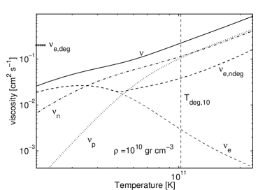
In fig. 5, we plot $\nu$ and its components as a fucntion of temperature. In the non-degenerate limit ($T>T_{\rm deg}$), protons and neutrons contribute equally to the total viscosity: they carry the same momentum density, transported in both cases by n-p collisions. In this regime, the electron contribution $\nu_{\rm e,ndeg}$ has been calculated as $\nu_{\rm e,ndeg}=\nu_{\rm S}\left(Y_{\rm e}\,\bar{v}_{\rm e}^{2}\,t_{\rm ep}/\bar{v}\,\lambda_{\rm ep,S}\right)$, where $Y_{\rm e}$ is the electron fraction and $t_{\rm ep}=0.15~{}{\rm sec}~{}T^{3/2}/n_{\rm p}\log\Lambda_{ep,S}$ (eq. 39 with $v=\bar{v}_{\rm e}$ and $p=\bar{v}_{\rm e}m_{\rm e}$). As the temperature decreases, the flow becomes neutron rich and the electrons degenerate. As this happens the proton momentum density drops faster than the neutron’s one, strong collisions with neutrons dominate the baryon collision frequency and the electron mean free path increases (while the baryon one keeps decreasing). As a consequence, electron viscosity becomes comparable or greater than the baryon viscosity. Since the electron density decreases with temperature, $\nu_{\rm e}$ eventually decreases (even if $\lambda_{\rm e}$ keeps increasing) and it does not attain the limiting viscosity value for strongly degenerate electrons (shown in the figure as the horizontal dashed line). Therefore the total viscosity $\nu$ decreases as the plasma cools even when electron viscosity dominates. The behaviour of $\nu$ as a function of density is shown in Figure 3. It decreases as the plasma becomes denser, since p-n collisions become more frequent and the electron (and thus their momentum) density decreases when below the nominal degeneracy temperature. In these figures, the $T<T_{\rm deg}$ regime represents the typical situation in hyper-accreting discs.

Figure 4 shows the predicted radial profile of the viscosity within the hyper-accreting disc models. In the optically thin regions of the disc the viscosity increases with radius, since the temperature in this region decreases much more slowly with radius than the density. Electron viscosity is higher than baryon viscosity but the two contributions tend to converge (and they can become comparable for low accretion rates) in the less dense regions away from the black hole where the electrons are less degenerate. The trend is the opposite in the optically thick innermost region, which is present only at high accretion rates. In this case the viscosity decreases moving outward. Here, the neutron contribution is highly suppressed ($\sim$ one-two orders of magnitude) and electrons completely dominate the flow viscosity.

8.1 Neutrino and photon viscosities

Photons and neutrinos can also in principle contribute to viscosity. In the case of neutrinos, the mean free path is of course enormous compared to that of the baryons, so momentum transport by neutrinos will dominate if it acts as a viscosity. This will depend upon the neutrino optical depth. In regions of the disc that are very optically thick neutrino viscosity will act as a (very large) Navier-Stokes viscosity. Indeed, Masada et al. (2007) have suggested that neutrinos might be able to shut off the MRI completely, by reducing the Reynolds number below that which admits linear growth of MRI modes. In optically thin regions, on the other hand, momentum transport by neutrinos is non-local and acts as a radiation drag rather than a viscosity (Arav & Begelman, 1992). In this paper we are principally concerned either with optically thin regions of the disc (where neutrinos do not contribute viscosity), or with regions of modest optical depth ($\tau_{\nu}\sim$ a few) for which the correct treatment is unclear. The reader should, however, bear in mind that the presence of neutrinos may have dynamical consequences in the optically thick regions of the flow. Since we derive high values of the Prandtl number while ignoring the neutrino contribution, to the extent that neutrinos contribute to viscosity, they will only reinforce our conclusions on the large Pm regime of hyper-accreting discs. Our magnetic Prandtl numbers are conservative in that sense.

The discussion on the different regimes according to the optical thickness also applies to photon viscosity. Our discs are everywhere in the mid-plane extremely optically thick to photons. This implies a much smaller mean free path for photons than for neutrinos and their contribution to viscosity is relatively suppressed by a factor equal to the ratio of mean free paths for the two species. Photon viscosity can also be neglected with respect to baryon viscosity, even if they have similar mean free paths, since the photon momentum density is small compared to the baryons’ one.

9 Comparison with X-ray binary discs

Figure 6: Comparison between the “X-ray binary” disc model and the “neutrino cooled” disc model for the electrical resistivity and the microscopic viscosity as a function of scaled radius. The “X-ray binary” disc has a $10M_{\sun}$ central object, $\dot{M}=0.1L_{\rm edd}/c^{2}$ (where the Eddington luminosity is $\sim 10^{39}$ erg s^-1) and $\alpha=0.01$. The neutrino cooled disc model has $\dot{M}=0.2\,M_{\sun}$sec^-1, $\alpha=0.1$ and $M_{\rm BH}=3\,M_{\odot}$.

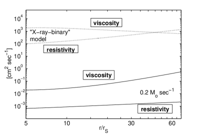
Identical methods can be used to compute the resistivity and viscosity for photon-cooled discs, which are present in X-ray binaries at similar radii around black holes of a few Solar masses. In Figure 6 we plot the radial profiles of these quantities for a model presented by Balbus & Henri (2007) as representative of a X-ray binary disc. The model has a central black hole of mass $10\ M_{\odot}$, surrounded by a disc accreting at one tenth the Eddington limit with $\alpha=0.01$. We treat the photon flux in the diffusion approximation, adopt an opacity that is of Kramers’ form plus an electron scattering correction ($\kappa\simeq 0.43+6.6~{}\rho T^{-7/2}$), and write the total pressure as the sum of the gas pressure (baryons and electrons) and photon pressure. The abundances are taken as 10% $\alpha$ particles and 90% hydrogen by number. The gas is completely ionised. In the X-ray binary regime the Spitzer resistivity (eq. 40) is valid (we neglect $e-\alpha$ collisions), while the viscosity is given by p-p Coulomb collisions and $\alpha$-p Coulomb collisions (see Appendix A in Balbus & Henri, 2008).

In the X-ray binary disc model the plasma is cooler and less dense, and electrons are non-degenerate. These characteristics enhance the e-p collision probability, resulting in a resistivity that is several orders of magnitude higher than in neutrino cooled discs. The viscosity is also much higher, and moreover, it decreases towards larger radii. This is the opposite trend to that seen for the viscosity in neutrino cooled discs.

10 The Magnetic Prandtl number

Figure 7: Magnetic Prandtl number as a function of scaled radius computed for the three neutrino cooled disc models shown in Figure 1. The magnetic Prandtl number for the ”X-ray binary” disc model is also shown for comparison, as a dotted curve.

With the results for the resistivity and viscosity in hand we can compute the magnetic Prandtl number, defined as the ratio of the microscopic viscosity to the resistivity,

$$\rm Pm=\frac{\nu}{\eta}.$$ (52)

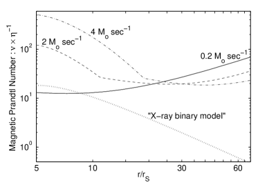
Results for the three disc models that we have discussed in detail are shown in Figure 7. The radial behaviour of $\rm Pm$ is mainly determined by the viscosity, since the resistivity is a rather weak function of radius. In optically thin regions of the disc (everywhere for $\dot{M}=0.2~{}M_{\sun}{\rm sec^{-1}}$, and at large radii, $r\lower 2.15277pt\hbox{$\;\buildrel>\over{\sim}\;$}15-30$ $r_{\rm S}$, for the higher accretion rate models) the $\rm Pm$ number is relatively flat but eventually increases with radius because the rapidly decreasing density increases the microscopic viscosity in the disc. In the optically thick regions, the temperature increases more rapidly toward the black hole than does the density, and the increased viscosity leads to larger $\rm Pm$ in the central parts. We note that, although the values of both the resistivity and the viscosity are far larger in the photon cooled X-ray binary disc model, the value of the magnetic Prandtl number is not all that different in these inner parts. More significant is the different radial behaviour. For hyper-accreting discs $\rm Pm$ increases with radius once the disc becomes optically thin, and this trend continues throughout the neutrino cooled zone. For X-ray binary discs $\rm Pm$ falls off with radius and eventually becomes smaller than one (at $r\sim 45$ r_g). Our results for this model are qualitatively similar to those of Balbus & Henri (2008) (see their fig. 1, left panel) with the quantitative differences arising due to different boundary conditions and value of $\eta_{\rm S}$.

Figure 8: Contours of magnetic Prandtl number in hyper-accreting discs as a function of radius and accretion rate, computed for $\alpha=0.01$.

Figure 9: The same as Figure. 8, but for $\alpha=0.1$.

Figure 10: The same as Figure. 8, but for $\alpha=1$.

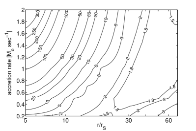
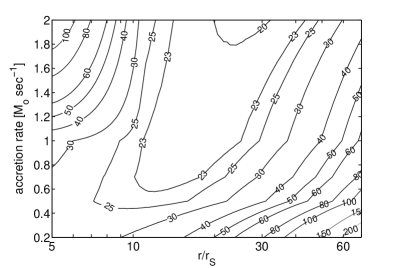
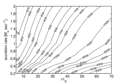
Figures 8, 9 and 10 show the dependence of $\rm Pm$ on radius and accretion rate for three different values of $\alpha$, $\alpha=0.01,0.1~{}{\rm and}~{}1$. We find that $\rm Pm>1$ throughout the neutrino cooled region for all accretion rates in the range $0.2\ M_{\odot}\ {\rm sec}^{-1}<\dot{M}<2\ M_{\odot}\ {\rm sec}^{-1}$. Typically $\rm Pm\gg 1$ (except in the $r>20r_{\rm S}$ regions for $\alpha=0.01$), with values as high as a few $10^{3}$ if $\alpha=1$.

As $\alpha$ decreases, the disc density is higher and the viscosity drops: the lower viscosity results in a smaller magnetic Prandtl number. This is unlike X-ray binary discs, where the $\alpha$ dependence of the microscopic viscosity is largely offset by a similar change in the resistivity (Balbus & Henri, 2008).

All the results discussed here are computed assuming midplane disc conditions. Moving toward the upper layers of the disc the density invariably drops more rapidly than the temperature, and as a consequence the electrons become non-degenerate. However, verticle mixing is efficient and the nuclear composition ($Y_{\rm p}$) at higher latitude is close to that at the midplane (Rossi, Armitage & Di Matteo, 2007). Under these conditions the resistivity increases more slowly than the viscosity (whose main contribution will be eventually come from neutrons) and $\rm Pm$ increases further.

11 Other non-ideal MHD effects

Our motivation for computing the magnetic Prandtl number derives from various suggestions that the saturation level of the MRI varies strongly with $\rm Pm$. Almost all numerical simulations addressing this issue include ohmic dissipation as the only non-ideal term in the MHD equations. If other non-ideal terms are dominant in hyper-accreting discs there will be (at the very least) additional uncertainties in interpreting the results of simulations for astrophysical discs. Here, we estimate the magnitude of the different non-ideal terms for fiducial values of temperature, $T=3\times 10^{10}$ K, and density, $\rho=5\times 10^{10}$ gr cm^-3. Under these conditions the plasma composition is $Y_{\rm p}\simeq 5.5\times 10^{-2}$, the chemical potential is $\mu=8.7$ and the sound speed $c_{\rm s}=1.6\times 10^{9}$ cm s^-1. The equipartition magnetic field,

$$B_{\rm eq}=\sqrt{8\pi\,P_{\rm b}}$$ (53)

is $1.8\times 10^{15}$ Gauss.

The low resistivity of plasma in neutrino cooled discs results in a very large magnetic Reynolds number. If we take $H=5.3\times 10^{6}$ cm ($\simeq 0.3\times 20~{}r_{\rm S}$), then

$$R_{\rm eM}=\frac{c_{\rm s}H}{\eta}\simeq 1.5\times 10^{19},$$ (54)

where we have used the consistent value of the resistivity $\eta=5.85\times 10^{-4}$ cm² s^-1. All non-ideal MHD effects are therefore small. In relative terms, however, the high density means that the plasma is sufficiently collisional that, for very weak magnetic fields, ohmic dissipation is stronger than both the Hall effect (the separation of charge carriers in the presence of a magnetic field perpendicular to the current) and ambipolar diffusion (the differential motion of neutrons and charged particles). The dominance of ohmic dissipation persists until the magnetic field becomes strong enough that the cyclotron frequencies of the charged particles exceed the collision frequencies. We can write the relative strength of the ohmic (O) and Hall (Ha) effects as (e.g. Sano & Stone, 2002),

$$\frac{\rm Ha}{\rm O}=\omega_{\rm ce}t_{\rm ep}.$$ (55)

where $\omega_{\rm ce}$ is the electron gyro-frequency and $t_{\rm ep}$ the e-p deflection timescale. For our conditions

$$t_{\rm ep}=\frac{\gamma_{e}}{4\pi r_{\rm e}\eta n_{-}}\simeq\frac{\mu+1}{3.54\times 10^{-12}\eta n_{p}}\simeq 2.87\times 10^{-18}{\rm sec},$$ (56)

where the electron density has been evaluated as $n_{-}\simeq n_{p}=\rho{Y_{\rm p}}/{m_{\rm p}}$, and

$$\omega_{\rm ce}=\frac{1.76\times 10^{7}}{\left<\gamma_{\rm e}\right>}\frac{\rm B}{\rm gauss}\,{\rm Hz},$$ (57)

where the mean Lorentz factor is $\gamma_{\rm e}\simeq\mu+1$. The field B here is the mean local field. Eq. 55 then gives, numerically,

$$\frac{\rm Ha}{\rm O}=5.2\times 10^{-12}\frac{\rm B}{\rm gauss}.$$ (58)

Likewise, the ratio of ambipolar (A) to Hall (H) strength can be written as (e.g. Sano & Stone, 2002),

$$\frac{\rm A}{\rm Ha}=\omega_{\rm cp}\;t_{\rm pn}\;(2-2Y_{\rm p})=9.4\times 10^{-17}\frac{\rm B}{\rm gauss},$$ (59)

where $\omega_{\rm cp}=\omega_{\rm ce}(\gamma_{e}m_{\rm e}/m_{\rm p})$ is the proton gyro-frequency and the p-n collision time-scale is $t_{\rm pn}=5.16\times 10^{-21}$ sec. We note again that the Coulomb coupling ($t_{\rm ep}$) is weaker than the strong collision coupling for our plasma conditions.

Eq. 55 and eq. 59 show that ohmic dissipation is the dominant non-ideal MHD term only in weakly magnetised plasmas which have a ratio of thermal to magnetic energy $\beta>10^{8}$. This means that, for any reasonable magnetic field in the disc, the Hall effect is the dominant non-ideal MHD effect. For our fiducial parameters the Hall effect becomes the most important non-ideal MHD effect for $B\lower 2.15277pt\hbox{$\;\buildrel>\over{\sim}\;$}2\times 10^{11}$ G. At equipartition ambipolar diffusion is also more important than resistive diffusion but we remain in the Hall regime.

12 The radiatively inefficient zone

In the outer disc — beyond $\sim$ one hundred $r_{\rm S}$ — the physical conditions are quite different. In this region the disc is photon-pressure dominated. The temperature ($T\lower 2.15277pt\hbox{$\;\buildrel<\over{\sim}\;$}10^{10}{\rm K}$) is below the neutrino cooling threshold and the flow is effectively non-radiative. The free baryons are in the form of $H_{\rm e}$ nuclei (Chen & Beloborodov, 2007) and the density ($\rho\lower 2.15277pt\hbox{$\;\buildrel<\over{\sim}\;$}10^{7}{\rm grcm^{-3}}$) is low enough that the electrons are non-degenerate (and non relativistic). The disc is thus both more resistive and more viscous, and the resistivity and viscosity have the classical Spitzer dependencies on temperature and density (eq. 40 and eq. 51) but with numerical coefficients (also in the “Spitzer” Coulomb logarithms eqs. 41 and 43) adjusted to be appropriate for a completely ionised He flow. It is worth emphasizing that unlike the radiatively inefficient flows discussed in the X-ray binary or AGN contexts (e.g Mahadevan & Quataert, 1997; Tanaka & Menou, 2006), those in hyper-accreting scenarios would remain fully collisional. This constitutes a rare situation in which the collisionality guarantees a unique temperature for electrons and nuclei. Moreover MHD dissipation scale arguments based on classical Spitzer values are adequate.

The magnetic Prandtl number in this region is,

$$\rm Pm=7.3\times 10^{-28}\frac{T^{4}}{\rho\Lambda},$$ (60)

where $\Lambda=\log{\Lambda_{\rm eHe}}\times\log{\Lambda_{\rm HeHe}}$ is the product of the Coulomb logarithm for $e-H_{\rm e}$ and for $H_{\rm e}-H_{\rm e}$ collisions.

If we assume that the temperature is set by a fraction of the virial energy density then $aT^{4}=f~{}(GM_{\rm bh}/r)\rho$. Numerically we find that $T^{4}/\rho=5.9\times 10^{34}f\left(r_{\rm S}/r\right)$ and

$$\rm Pm\simeq\frac{1.44\times 10^{6}}{(\Lambda/15)}\left(\frac{r_{\rm S}}{r}\right),$$ (61)

where we take $f=1/2$ . $\Lambda$ varies very slowly with radius and eq. 61 with $(\Lambda/15)=1$ is actually a very good approximation for $\rm Pm$ in the whole outer disc. We note that $\rm Pm\gg 1$ and it falls off slowly as $r^{-1}$: for $r\lower 2.15277pt\hbox{$\;\buildrel>\over{\sim}\;$}100r_{\rm S}$, $\rm Pm\lower 2.15277pt\hbox{$\;\buildrel<\over{\sim}\;$}10^{4}$.

This result indicates that in the outer regions of hyper-accreting discs $\rm Pm$ has a very different behaviour than in the innermost parts. Here $\rm Pm$ is rather insensitive to the actual accreting conditions $\dot{M}$ and $\alpha$ (as long as the outer disc remains photon-pressure dominated), but it is a stronger function of temperature and it decreases with radius. However, both regions have in common $\rm Pm>1$: unlike X-ray binary and AGN discs, hyper-accreting discs seem not to have a $\rm Pm<1$ region. Beside a high $\rm Pm$, this outer disc flow has other characteristics in common with the neutrino-cooled region. The conductivity is high with $R_{\rm eM}\sim 10^{12}-10^{11}$ and the Hall effect dominates even for modest magnetic fields ($\beta<10^{6}-10^{5}$). These features are caused by the still high temperature that makes Coulomb coupling rather inefficient (though in the outer region it is still more efficient than nuclear coupling).

13 Discussion

In this section, we attempt to relate the plasma properties that we have computed to the global properties of discs. There are many steps required to connect the microscopic scales where resistivity and viscosity act to the global evolution of the disc, and simulations and analytic arguments provide only an imperfect guide. However, plausible guesses are possible. We focus on the possible consequences of magnetic Prandtl number greater than unity for the magnetisation and evolution of hyper-accreting discs.

Let us first summarise the argument that suggests that the magnetic Prandtl number matters. In turbulent plasmas with $\rm Pm>1$, the absence of turbulence below the viscous scale $\lambda_{\nu}\sim R_{\rm e}^{-3/4}H$ means that the resistive scale may not be easily accessible to field lines and reconnection could be slow with respect to magnetic amplification. We can understand the dependence on $\rm Pm$ with the following simple argument. Turbulence at scale $\lambda_{\nu}$ exponentially amplifies the magnetic field on an eddy turnover time-scale $t_{\rm eddy}=H/c_{\rm s}\left(\lambda_{\nu}/H\right)^{2/3}$, while the magnetic field dissipation on that same scale takes $t_{\eta}=\lambda_{\nu}^{2}/\eta$. The ratio of these timescales is

$$\frac{t_{\eta}}{t_{\rm eddy}}\simeq\rm Pm.$$ (62)

So, for $\rm Pm>1$, magnetic energy can build up, first on the viscous scale and subsequently in an upward cascade toward larger scales (Brandenburg, 2001).

This may have important consequences for accretion discs. Within discs, the turbulent growth of magnetic fields can be limited – in principle – by either resistive dissipation (on small scales) or buoyant expulsion of the flux from the disc. Numerical simulations suggest that in low $\rm Pm$ discs resistive dissipation ultimately sets the saturation level (e.g. Stone et al., 1996). If, however, the small-scale dissipation of magnetic fields is frustrated by a high magnetic Prandtl number, the only channel available to limit the flux may be macroscopic buoyancy. Since buoyancy is relatively inefficient – the timescale is likely to modestly exceed the Alfvén crossing time $H/V_{\rm A}$ of the disc – a high magnetic Prandtl number disc could saturate at a level that involves stronger magnetic fields, more vigorous turbulence and angular momentum transport, and ongoing field expulsion. These expectations are supported by the available numerical evidence. Lesur & Longaretti (2007) and Fromang et al. (2007) find that the parameter $\alpha$ increases with the magnetic Prandtl number in the range $2\leq\rm Pm\leq 8$ and $R_{\rm e}\sim 10^{3}-10^{4}$. In the case where $\alpha$ approaches unity, Lesur & Longaretti (2007) find a highly time dependent disc, with large fluctuations in $\alpha$ and the mean magnetic pressure. This appears to be a consequence of the well-known dependence of the strength of the MRI on the magnetic field: as the ratio $\beta$ of thermal to magnetic pressure decreases $\alpha$ at first increases until the MRI is quenched around equipartition (Hawley, Gammie & Balbus, 1995; Lesur & Longaretti, 2007).

Based on these arguments, two evolutionary consequences can be contemplated for hyper-accreting discs formed after stellar core collapse or compact object mergers. In the initial phase, a high magnetic Prandtl number in the neutrino cooled inner disc results in stronger magnetic field and a higher efficiency of angular momentum transport. Since, as we have shown, a higher $\alpha$ in such discs results in a yet higher $\rm Pm$, a runaway occurs until $\alpha\sim 1$. This regime is sustainable for many dynamical timescales, provided that the excess magnetic energy that could quench the MRI is removed from the disc, for example, by buoyancy. This is plausible since close to equipartition the buoyancy timescale $\sim H/V_{\rm A}\sim\Omega^{-1}$ is similar to the orbital timescale and can provide cooling by removing magnetic energy. The disc, which would be in a similar regime to that simulated by Lesur & Longaretti (2007), would be highly variable. This initial stage, in which a highly variable magnetic “corona” is built above the disc via flux expulsion, could be associated with the production of a magnetic outflow, dynamically similar to those studied by Proga et al. (2003) and McKinney (2006) (see also King et al., 2004), polluted with some disk matter, that eventually will be observed as a GRB.

The longer term evolution of very high $\rm Pm$ discs is less clear. One possibility is that eventually a net vertical field, which cannot be removed locally by buoyancy, builds up and suppresses the MRI. This depends upon the ability of field lines to diffuse outwards. Turbulent diffusion can depend in turn on the strength of the magnetic field and on non-linear MHD effects. In our case the dominance of the Hall effect may influence the behaviour of the turbulence, by introducing an asymmetry between magnetic fields that are aligned or anti-aligned with the direction of the angular momentum vector (Sano & Stone, 2002). The outcome is thus uncertain and the investigation requires numerical methods.

From a purely phenomenological perspective, one might note that there are similarities between the state transitions in X-ray binaries and GRB prompt and late-time activity. Our results show the presence of a high $\rm Pm$ number inner region in both discs. One may then speculate that the GRB prompt phase could involve similar physical conditions, insofar the magnetic field behaviour is concerned, to the transition to the “low/hard state” in X-ray binaries, which is observationally associated with the emergence of an outflow (Fender et al., 1999). However, the theoretical analogy with X-ray binaries is imperfect, since it is unclear that what causes a change in state may be the same physical mechanism in both sources. For X-ray binary discs the temperature dependence of $\rm Pm$ may allow a local thermal runaway, and it has been suggested that this ultimately causes global state transitions (Balbus & Henri, 2008). The conditions for such a mechanism to work in hyper-accreting discs are present only in the outer radiatively inefficient regions, since in the neutrino-cooled regions $\rm Pm$ is primarily a function of density. However, a classical thermal instability is not possible in radiatively inefficient flows.

14 Conclusions

In this paper, we calculated the magnetic Prandtl number for plasma conditions in hyper-accreting discs. This dimensionless number $\rm Pm=\nu/\eta=\lambda_{\nu}^{2}/\lambda_{\eta}^{2}$ expresses the relative size of two critical turbulent flow scales: the scale on which velocity fluctuations are viscously damped $\lambda_{\nu}$, and the scale $\lambda_{\eta}$ on which ohmic losses result in magnetic field dissipation. We find that in the inner neutrino-cooled regime:

• Electric resistivity involves relativistic, mildly degenerate electrons. As a consequence, the resistivity is very low and weakly dependent on density and temperature.

• The main source of viscosity is Coulomb collisions between mildly degenerate electrons and protons. It decreases as the flow gets denser or cooler, since the electron fraction decreases.

• The magnetic Prandtl number is always greater than unity, unless the angular momentum transport efficiency, parameterized via the Shakura-Sunyaev $\alpha$, is very small ($\alpha<0.01$). $\rm Pm$ ranges between a few tens to a few $10^{3}$, and it typically increases with $\alpha$. In the optically thin regions for neutrinos, the main dependence of $\rm Pm$ is on density (inversely, via viscosity) since the disc temperature varies very slowly as a function of $\dot{M}$ and radius. This causes $\rm Pm$ to decrease with increasing accretion rates. In the optically thick regions, the main dependence is on temperature, that varies more rapidly than density. As a consequence, $\rm Pm$ increases with $\dot{M}$

In the outer, radiatively inefficient region:

• Resistivity and viscosity have the classical “Spitzer” dependencies on temperature and density, since electrons are non-relativistic and non-degenerate and viscosity is mainly given by Coulomb interactions between ionised helium particles. The magnetic Prandtl number is thus a much stronger function of temperature $\rm Pm\propto T^{4}/\rho$. In contrast, it does not depend on the overall magnitude of accretion (via $\dot{M}$ and $\alpha$). The Prandtl number is always much larger than unity ($\rm Pm\simeq 10^{4}(100~{}r_{\rm S})/r$) and it is unlikely to fall below unity for the entire extent of the disc.

We conclude by noting a number of implications for the global structure of hyper-accreting discs:

• For all plausible values of the magnetic field strength in the disc, the Hall effect provides the largest non-ideal term in the MHD equations. These discs are perhaps a unique example of a high magnetic Reynolds number flow in which the Hall effect is the dominant non-ideal term. Since there are no simulations where these conditions are accounted for, their effect on the magnetic field evolution and MRI is unclear.

• The large values of the magnetic Prandtl number mean that the evolution of magnetic field within hyper-accreting discs is likely to be qualitatively different from discs with lower magnetic Prandtl numbers. The results of forced dynamo and MRI simulations suggest that, in the high $\rm Pm$ regime, small scale field dissipation is suppressed and the saturation level of the magnetic field is enhanced, perhaps dramatically (Lesur & Longaretti, 2007; Fromang et al., 2007). Numerical simulations of hyper-accreting discs that do not account for microphysical dissipation may therefore have underestimated the magnetic field strength.

• The immediate consequence of a high value of $\rm Pm$ for models of the central engines of GRBs is that disc formation is likely to be accompanied by vigorous expulsion of magnetic flux. This favours models in which energy is liberated in the form of a magnetic jet or outflow.

References

- Arav & Begelman (1992) Arav, N. & Begelman, M.C. 1992, ApJ 401, 125
- Balbus & Hawley (1998) Balbus, S. A., Hawley, J. F. 1998, Reviews of Modern Physics, 70, 1
- Balbus & Henri (2008) Balbus, S. A., & Henri, P. 2008, ApJ , 674, 408
- Bethe (1949) Bethe, H.A. 1949, Phys.Rev., 76, 38
- Beloborodov (2003) Beloborodov, A. M. 2003, ApJ ,588, 944
- Blandford & Payne (1982) Blandford, R. D., Payne, D. G. 1982, MNRAS, 199, 883
- Brandenburg (2001) Brandenburg, A. 2001, ApJ, 550, 824
- Braginskii (1957) Braginskii, S. I. 1957, J.Exptl.Theoret.Phys.,33,459
- Braginskii (1958) Braginskii, S. I. 1958, Soviet Phys. JETP, 6,358
- Burrows et al. (2005) Burrows, D. N. et al. 2005, Sci, 309, 1833
- Chen & Beloborodov (2007) Chen, W-X, & Beloborodov A.M. 2007, ApJ , 657:383
- Di Matteo, Perna & Narayan (2002) Di Matteo, T., Perna, R., Narayan, R., 2002, ApJ , 579, 706
- Fender et al. (1999) Fender, R. et al. 1999,ApJ , 519, 165
- Fromang et al. (2007) Fromang, S., Papaloizou, J., Lesur, G., & Heinemann, T. 2007, A&A, 476, 1123
- Hackenburg (2006) Hackenburg, H., 2006, PRC, 73, 044002
- Hawley, Gammie & Balbus (1995) Hawley, J. F., Gammie, C. F., & Balbus, S. A. 1995, ApJ , 440, 742
- King et al. (2004) King, A. R., Pringle, J. E., West, R. G., Livio, M., 2004, MNRAS , 348, 111
- Kohri & Mineshige (2002) Kohri, K., & Mineshige, S. 2002, ApJ , 577, 311
- Lesur & Longaretti (2007) Lesur, G., & Longaretti, P.-Y. 2007, MNRAS, 378, 1471
- Lynden-Bell & Pringle (1974) Lynden-Bell, D. & Pringle, J. E. 1974, MNRAS , 168, 603
- Longair (1992) Longair, M. S., “High Energy Astrophysics”, 1992, Cambridge University Press
- Mahadevan & Quataert (1997) Mahadevan, R. & Quataert, E., 1997, ApJ , 490, 605
- Masada et al. (2007) Masada, Y., Kawanaka, N., Sano, T., & Shibata, K. 2007, ApJ , 663, 437
- McKinney (2006) McKinney, J. C. 2006, MNRAS , 368, 1561
- Miller et al. (1990) Miller,G. A.,Nefkens, B.M.K., & Šlaus, I. 1990, PhR, 194, 1
- Nandkumar & Pethick (1984) Nandkumar, R. & Pethick, C. J., MNRAS , 209, 511
- Narayan, Piran & Kumar (2001) Narayan, R., Piran, Tsvi, & Kumar, P., 2001, ApJ , 557, 949
- Popham, Woosley & Fryer (1999) Popham, R., Woosley, S. E., & Fryer, C. 1999, ApJ , 581,356
- Potekhin (1999) Potekhin, A.Y 1999, A&A , 351, 797
- Potekhin et al. (1999) Potekhin, A.Y, Baiko, D.A., Haensel, P., & Yakovlev, D.G. 1999, A&A , 351, 797
- Pringle (1981) Pringle, J. E. 1981, ARA&A, 19, 137
- Proga et al. (2003) Proga, D., MacFadyen, A. I., Armitage, P. J., & Begelman, M. C. 2003, ApJ , 599, L5
- Rossi, Armitage & Di Matteo (2007) Rossi, E. M., Armitage, P. J. & Di Matteo, T., 2007, Ap&SS, 311, 185
- Ruffert & Janka (1999) Ruffert, M. & Janka, H.-T.1999, A&A , 344, 573
- Sano & Stone (2002) Sano, T., & Stone, J. M., 2002, ApJ , 570, 314
- Schekochihin et al. (2004) Schekochihin, A. A., Cowley, S. C., Taylor, S. F., Maron, J. L., & McWilliams, J. C. 2004, ApJ, 612, 276
- Shakura & Sunyaev (1973) Shakura, N. I., & Sunyaev, R. A. 1973, A&A, 24, 337
- Spitzer (1962) Spitzer, L. 1962, Physics of Fully Ionized Gases, New York: Interscience (2nd edition)
- Spruit, Stehle & Papaloizou (1995) Spruit, H. C., Stehle, R., & Papaloizou, J. C. B. 1995, MNRAS , 275, 1223
- Stone et al. (1996) Stone, J.M., Hawley, J.F., Gammie, C.F., & Balbus, S.A. 1996, ApJ , 463,656
- Tanaka & Menou (2006) Tanaka, T., & Menou, K., 2006, ApJ , 649, 345
- Umurhan, Menou & Regev (2007a) Umurhan, O. M., Menou, K., & Regev, O. 2007a, PRL 98, 034501
- Umurhan, Regev & Menou (2007b) Umurhan, O. M., Regev, O. & Menou, K. 2007b, PRE 76, 036310
- Woosley (1993) Woosley, S. E. 1993, ApJ, 405, 273