Gap solitons in a model of a superfluid fermion gas in optical lattices

Abstract

We consider a dynamical model for a Fermi gas in the Bardeen-Cooper-Schrieffer (BCS) superfluid state, trapped in a combination of a 1D or 2D optical lattice (OL) and a tight parabolic potential acting in the transverse direction(s). The model is based on an equation for the order parameter (wave function), which is derived from the energy density for the weakly coupled BCS superfluid. The equation includes a nonlinear self-repulsive term of power $7/3$, which accounts for the Fermi pressure. Reducing the equation to the 1D or 2D form, we construct families of stable 1D and 2D gap solitons (GSs) by means of numerical simulations, which are guided by the variational approximation (VA). The GSs are, chiefly, compact objects trapped in a single cell of the OL potential. In the linear limit, the VA predicts almost exact positions of narrow Bloch bands that separate the semi-infinite and first finite gaps, as well as the first and second finite ones. Families of stable even and odd bound states of 1D GSs are constructed too. We also demonstrate that the GS can be dragged without much distortion by an OL moving at a moderate velocity ($\sim$ 1 mm/s, in physical units). The predicted GSs contain $\sim 10^{3}-10^{4}$ and $\sim 10^{3}$ atoms per 1D and 2D settings, respectively.

1 Introduction

Studies of matter-wave patterns in degenerate Bose [1] and Fermi [2] gases at ultra-low temperatures have drawn a great deal of attention in the last decade. The theoretical description of patterns formed in a Bose-Einstein condensate (BEC) relies upon the Gross-Pitaevskii equation (GPE), which produces a remarkably accurate description of various states, including solitons [3]. Experimentally, bright matter-wave solitons were created in BEC of ⁷Li [4] and ⁸⁵Rb atoms [5]. In either case, the interaction between the atoms was switched from repulsion to attraction by means of the magnetic field applied near the respective Feshbach resonance (FR) [6, 7]. In BEC with repulsion between atoms, loaded in a periodic optical-lattice (OL) potential, which can be created as a standing wave by counter-propagating laser beams illuminating the condensate, localized states can be formed in the form of gap solitons (GSs). This was predicted taking into consideration the possibility of having a negative effective mass in parts of the bandgap spectrum induced by the periodic potential [8, 9]. GSs are supported by the interplay of the negative effective mass and repulsive nonlinearity. They are stable against small perturbations [10]. The prediction was followed by the creation of a GS formed by $\simeq 250$ atoms of ⁸⁷Rb in a nearly one-dimensional (1D), i.e., “cigar-shaped”, cross-beam optical trap, combined with the longitudinal OL potential [11, 12]. In the experiment, the gas was subjected to acceleration, in order to push atoms into a state with a negative effective mass. Other theoretically elaborated possibilities for the creation of GSs rely on the phase-imprinting method [13], or on temporarily adding a strong parabolic trap to the OL potential, with the objective to squeeze the condensate into a small region and then, relaxing the trap, to give the condensate a chance to self-trap into a compact GS state [14].

The creation of degenerate Fermi gases (DFG), and observation of the transition to Bardeen-Cooper-Schrieffer (BCS) superfluidity in them [15], suggest to consider possibilities of the creation of solitons in DFGs and BCS superfluids. Bright solitons were also predicted in Fermi-Bose mixtures with repulsion [16, 17] or attraction [17] between bosons and strong attraction between fermions and bosons.

A possibility of the existence of fermionic GSs was mentioned in work [18], in relation to a model of a binary boson condensate trapped in a one- or two-dimensional OL, with repulsion between the two components and zero intra-species interaction, as the respective system of coupled GPEs may also be realized as a system of equations for two fermionic wave functions, and thus the GSs reported in [18] may be interpreted as 1D and 2D symbiotic two-component GSs in the binary DFG (term “symbiotic” is frequently applied to two-component solitons in situations when each component in isolation is not able to form a soliton, while the coupling between them makes it possible [19]). Using more sophisticated models, one-dimensional GSs in the Fermi-Bose mixture with a small number of Bose atoms were predicted [20], and a possibility to create solitons in a mixed 1D Bose-Fermi superfluid composed of a relatively small number of atoms was proposed in [21].

In the strictly 1D geometry, the DFG can be mapped into the Tonks-Girardeau gas of hard-core bosons [22], which, in a certain approximation, may be described by the 1D nonlinear Schrödinger (NLS) equation with a repulsive quintic term [23]. In works [24], GSs were predicted in the latter equation which includes the OL potential, although the solitons reported in those works may be unstable against small perturbations.

In this work, we aim to predict 1D and 2D GSs in a BCS superfluid, which may be formed by Fermi atoms with weak attraction between ones with opposite orientations of the atomic spin. The GSs will be found, chiefly, in the form of tightly bound states, localized in a single cell of the OL potential. A rigorous many-body approach to the dynamics of the DFG, based on the system of quantum-mechanical equations of motion for individual fermions, made it possible to demonstrate the formation of fermionic GSs in a Bose-Fermi mixture [25]. However, such a microscopic approach becomes unfeasible as the number of fermions increases. A simplified dynamical model of the BCS superfluid relies on the use of a single wave function for fermions bound into Cooper pairs. This approach may be compared to that adopted in the Ginzburg-Landau theory, where the wave function describing the Fermi superfluid is introduced as a phenomenological complex order parameter [26]. Actually, the so developed description of macroscopic objects, such as solitons, is valid in the hydrodynamic approximation, i.e., under the condition that the solitons’ size is much larger than the de Broglie wavelength at the Fermi surface, in terms of the underlying microscopic distribution of the fermion atoms. As a result, the wave function of the BCS superfluid loaded in the 1D or 2D OL, and confined in the remaining (transverse) direction(s) by a tight “cigar-shaped” or “pancake” trap, obeys, respectively, the 1D or 2D Schrödinger equation, which includes the corresponding OL potential and a repulsive nonlinear term of power $7/3$ [27]. The equation is derived from the Lagrangian which includes the energy density for the weakly-coupled BCS superfluid, as obtained in well-known works [28].

We construct GS solutions by means of numerical computations, which are guided by an analytical variational approximation (VA) [29]; this approach has produced very accurate results in a model of the Bose-Fermi superfluid mixture [30]. The stability of the GSs is established in a numerical form, through direct simulations of the evolution of perturbed solitons. We conclude that the VA performs well in describing profiles of compact fundamental GSs sufficiently deep in bandgaps, but it works poorly near bandgap edges, facing the difficulty in reproducing undulating tails demonstrated by numerical simulations in that case. In the linear limit, the approximation very accurately predicts the location of the left edge of the first finite bandgap.

The paper is organized as follows. The derivation of the 1D and 2D equations for the wave function is presented in Section II. In Section III, we construct a family of stable fundamental GS solutions in the first two finite bandgaps of the 1D model, using the VA based on the Gaussian ansatz and direct numerical solutions. The GS solutions maintain a tightly-bound (compact) shape, unless their chemical potential is taken very close to edges of the bandgaps. In Section III, we also present stable symmetric and antisymmetric bound states of fundamental GSs, and consider a possibility of dragging GSs by a moving OL potential. In the framework of the GPE, the latter issue has drawn considerable attention as a means for transportation of matter-wave solitons, see work [31] and references therein. In Section IV, we report variational and numerical results for stable GSs in the 2D equation. In addition to the case of the square-lattice potential, in Section IV we also find 2D radial GSs, supported by an axisymmetric potential which is periodic along the radius (in BEC trapped in the axisymmetric OL, radial GSs have been predicted in work [32]). Estimates for the number of atoms in the predicted 1D and 2D GSs are given at the end of Sections III and IV, respectively, the result being $N_{\mathrm{1Dsoliton}}\sim 10^{3}-10^{4}$ and $N_{\mathrm{2Dsoliton}}\simeq 2,000$.

For the sake of comparison, in Sections III and IV we additionally display variational and numerical results for GS families in the ordinary GPE-based 1D and 2D models, which include the corresponding OL potential and, respectively, the cubic or quintic self-repulsive term. Actually, the accuracy provided by the VA in the model with the present model, with the nonlinearity of power $7/3$, is higher than in the models with the cubic or quintic nonlinear terms.

In addition to the spatially symmetric (even) fundamental GSs, the 1D equation gives rise to subfundamental (SF) solitons, which are localized odd states originating in the second bandgap. The SF solitons are also squeezed, essentially, into a single cell of the OL potential, but unlike the fundamental GSs, they are (weakly) unstable. The SF solitons are considered in Appendix. In particular, the VA developed for them yields a physically relevant finding: in the linear limit, it accurately predicts the position of the narrow Bloch band separating the first and second bandgaps.

2 Dynamical Equations

2.1 The equation in the general form

We consider a BCS superfluid of Fermi atoms with spin $1/2$ and mass $m$, assuming weak attraction between fermions with opposite orientations of the spin. To derive an effective equation for the superfluid order parameter, we start with the well-known expression for the energy density of the weakly coupled BCS superfluid in the 3D space [28, 33],

$$\mathcal{E}_{\mathrm{3D}}=(3/5)\rho_{\mathrm{3D}}\varepsilon_{F}+4\pi a\hbar^{2}\rho_{\mathrm{3D}}^{2}/(2m)+...,$$ (1)

which is built as an expansion in powers of $k_{F}a$, where $\hbar k_{F}$ and $a$ are the Fermi momentum and scattering length of the weak interaction between fermions in the BCS limit, $\varepsilon_{F}=\left(\hbar k_{F}\right)^{2}/(2m)$ is the Fermi energy, and $\rho_{\mathrm{3D}}$ the atomic density. The second term in Eq. (1) is a small correction to the first one due to the underlying condition, $k_{F}a\ll 1$ (which actually implies that $a$ is much smaller than the de Broglie wavelength at the Fermi surface). Taking into regard the Cooper pairing of spin-up and spin-down fermions, their total density is $\rho_{\mathrm{3D}}={2(2\pi)^{-3}}\int_{0}^{k_{F}}4\pi k^{2}dk\equiv\left(3\pi^{2}\right)^{-1}\left(2m\varepsilon_{F}/\hbar^{2}\right)^{3/2}$. From here, the Fermi energy can be expressed in terms of the atom density,

$$\varepsilon_{F}=\frac{\hbar^{2}}{2m}\left(3\pi^{2}\rho_{\mathrm{3D}}\right)^{2/3},$$ (2)

hence the energy density in Eq. (1) is cast in the form of

$$\mathcal{E}_{\mathrm{3D}}=\frac{3(3\pi^{2})^{2/3}\hbar^{2}}{10m}\rho_{3D}^{5/3}+\frac{2\pi a\hbar^{2}}{m}\rho_{\mathrm{3D}}^{2},$$ (3)

which includes the lowest-order correction proportional to scattering length $a$.

In the framework of the density-functional theory, the BCS superfluid is described by a complex order parameter (wave function), $\Psi$, such that $\rho_{\mathrm{3D}}\equiv|\Psi|^{2}$. If the Fermi energy is much larger than the depth of the external potential, $V(\mathbf{r})$, the evolution of the order parameter can be derived from the corresponding Lagrangian density which includes energy density (3),

$$\mathcal{L} = \frac{i\hbar}{2}(\Psi^{\ast}\Psi_{t}-\Psi\Psi_{t}^{\ast})-\frac{\hbar^{2}}{2m_{\mathrm{eff}}}|\nabla\Psi|^{2}-V(\mathbf{r})|\Psi|^{2}$$ (4)

$$-\frac{3(3\pi^{2})^{2/3}\hbar^{2}}{10m}|\Psi|^{10/3}-\frac{2\pi a\hbar^{2}}{m}|\Psi|^{4},$$

where $m_{\mathrm{eff}}$ is the effective mass of the order-parameter field in the density-functional theory, which determines the gradient term in the Lagrangian density. Such a formalism has been used in the description of Fermi superfluids in various contexts [34].

The Euler-Lagrange equation which follows from the full Lagrangian, $L=\int\mathcal{L}d\mathbf{r}$, where density (4) is inserted, takes the form of the three-dimensional NLS equation with the repulsive nonlinear term of power $7/3$, and a small correction in the form of the cubic term:

$$i\hbar\Psi_{t}=-\frac{\hbar^{2}}{2m_{\mathrm{eff}}}\left(\partial_{x}^{2}+\partial_{y}^{2}+\partial_{z}^{2}\right)\Psi$$

$$+\frac{\hbar^{2}}{2m}\left[\left(3\pi^{2}\right)^{2/3}|\Psi|^{4/3}+8\pi a|\Psi|^{2}\right]\Psi+V(\mathbf{r})\Psi.$$ (5)

Since $|\Psi|^{2}$ is defined as the atomic density, Eq. (5) is supplemented by the normalization condition,

$$\int\int\int|\Psi(\mathbf{r},t)|^{2}dxdydz=N,$$ (6)

where $N$ is the total number of atoms.

Equation (5), which was derived from the local Fermi distribution, applies to the description of spatially nonuniform patterns in the hydrodynamic limit, which assumes that the nonuniformity does not strongly disturb the local distribution. To say it more accurately, the hydrodynamic approach is valid if the characteristic size of the macroscopic pattern (actually, the width of the soliton, which is close to the OL period, $\lambda/2$, see Fig. 2 below) is much larger than the de Broglie wavelength at the Fermi surface, i.e.,

$$\lambda\gg 2\pi/k_{F}.$$ (7)

This condition is similar to that necessary for the validity of the hydrodynamic approximation in classical rarefied gases: the scale of the flow must be much larger that the free-path length.

2.2 The one-dimensional equation

Taking $V(\mathbf{r})$ as the potential of the 3D OL, Eq. (5) can be used to construct three-dimensional GSs. However, producing systematic results for 3D solitons is a challenging numerical problem. In this work, our objective is to reduce the equation to its 1D and 2D forms, assuming, as mentioned above, that the superfluid is held in a relatively tight cigar-shaped or pancake-like trap, that correspond to the following transverse potentials:

$$V_{\perp}^{\left(\mathrm{cig}\right)}=\frac{1}{2}m\omega_{\perp}^{2}\left(y^{2}+z^{2}\right);V_{\perp}^{\left(\mathrm{panc}\right)}=\frac{1}{2}m\omega_{\perp}^{2}z^{2}.$$ (8)

For this reduction to be valid, the Fermi energy must be larger than both the distance between energy levels in the spectra of harmonic-oscillator potentials (8), and depth $V_{0}$ of the longitudinal OL potential:

$$\varepsilon_{F}\gg\hbar\omega_{\perp},V_{0}~{}.$$ (9)

Equations (7) and (9) constitute conditions necessary for the validity of the approach elaborated in the present work.

The next step is reducing Eq. (5) to effective 1D and 2D equations. In the ordinary GPE with the cubic nonlinearity, the reduction of the 3D equation to its 1D and 2D forms can be performed in different ways, depending on the particular setting [35, 36, 37]. In the simplest situation, the reduction of the 3D equation to 1D starts with assuming the factorization of the wave function,

$$\Psi(x,y,z,t)=\Phi(x,t)\exp\left(-\frac{y^{2}+z^{2}}{2na_{\mathrm{ho}}^{2}}\right),$$ (10)

where the transverse harmonic-oscillator length is $a_{\mathrm{ho}}=\sqrt{\hbar/\left(m\omega_{\perp}\right)}$, and, in the case of a very tight confinement, $n=1$. However, due to condition (9), $\varepsilon_{F}$ corresponds not to the ground state of the transverse potential, but rather to an excited state with large quantum number $n$, so that $\varepsilon_{F}=n\hbar\omega_{\perp}$, and the transverse size of the domain filled by the Fermi superfluid is $\simeq\sqrt{n}a_{\mathrm{ho}}$. Accordingly, the second multiplier in Eq. (10) approximates a lumped superposition of excited states of the transverse harmonic oscillator, with the corresponding quantum number taking values from $1$ to $n$. The self-consistency demands that $\varepsilon_{F}=n\hbar\omega_{\perp}$, which, after a simple analysis, leads to relation

$$2n=\left((3/2)\pi^{2}\rho_{\mathrm{3D}}a_{\mathrm{ho}}^{3}\right)^{2/3}.$$ (11)

One-dimensional function $\Phi(x,t)$ in ansatz (10)  accounts for the dynamics in the $x$ direction, its normalization being determined by Eq. (6). The substitution of Eq. (10) in Eq. (5) and subsequent averaging of the 3D equation in the transverse plane yield the effective 1D equation

$$i\hbar\Phi_{t} = -\frac{\hbar^{2}}{2m_{\mathrm{eff}}}\Phi_{xx}+\left(\frac{3}{2}\pi^{2}\right)^{2/3}\frac{3\hbar^{2}}{{10}m}|\Phi|^{4/3}\Phi$$ (12)

$$+\frac{\pi a\hbar^{2}}{m}|\Phi|^{2}\Phi-\epsilon\cos\left(\frac{4\pi}{\lambda}x\right)\Phi,$$

where the 1D potential with strength $-\epsilon$ corresponds to the OL with period $\lambda/2$ (the negative sign in front of $\epsilon$ implies that a local minimum of the potential is set at $x=0$, where the center of the soliton will be placed).

By means of rescaling

$$\Phi\equiv\sqrt{\frac{2N}{n\lambda}}a_{\mathrm{ho}}^{-1}{\psi},~{}t=\frac{m_{\mathrm{eff}}\lambda^{2}}{4\pi^{2}\hbar}\tilde{t},~{}x\equiv\frac{\lambda}{2\pi}\tilde{x},$$ (13)

Eq. (12) is cast in the dimensionless form,

$$i\psi_{t} = -\frac{1}{2}\psi_{xx}+G_{\mathrm{1D}}^{(7/3)}|\psi|^{4/3}\psi$$ (14)

$$+g_{\mathrm{1D}}|\psi|^{2}\psi-V_{0}\cos\left(2x\right)\psi$$

(tildes are dropped here), with the rescaled 1D wave function subject to normalization

$$\int_{-\infty}^{+\infty}\left|\psi(x)\right|^{2}dx=1.$$ (15)

The effective strengths of the Fermi nonlinearity, weak cubic interaction, and OL potential are defined here as follows:

$$G_{\mathrm{1D}}^{(7/3)} \equiv \frac{{3}}{{10}}\frac{m_{\mathrm{eff}}}{m}\left(\frac{{3}\lambda^{2}N}{{8}\pi na_{\mathrm{ho}}^{2}}\right)^{2/3},~{}~{}$$

$$V_{0} \equiv m_{\mathrm{eff}}\left(\frac{\lambda}{2\pi\hbar}\right)^{2}\epsilon,\quad~{}g_{\mathrm{1D}}=\frac{m_{\mathrm{eff}}}{m}\frac{a\lambda N}{2\pi na_{\mathrm{ho}}^{2}}~{}.$$ (16)

Actually, $V_{0}$ is the OL depth measured in units of the recoil energy, $E_{R}=(2\pi\hbar)^{2}/(2m\lambda^{2})$. Below, it will be demonstrated that $G_{\mathrm{1D}}^{(7/3)}$ takes values $\lesssim 10$ (see Fig. 2), while $g_{\mathrm{1D}}$ is confined to the range of $\sim 10^{-3}$, hence the cubic term may be safely neglected in the first approximation.

2.3 The two-dimensional equation

Under the transverse confinement in direction $z$, which corresponds to the “pancake” configuration, Eq. (5) can be reduced to a 2D form in the plane of $\left(x,y\right)$. To this end, following [35], we substitute $\Psi(x,y,z,t)=\Phi(x,y,t)\exp\left(-z^{2}/\left(2na_{\mathrm{ho}}^{2}\right)\right)$, cf. Eq. (10). Averaging in $z$ and making use of the same rescalings as in Eq. (13), except for a different transformation of the wave function,

$$\Phi\equiv\frac{2\pi^{3/4}\sqrt{N}}{n^{1/4}\lambda\sqrt{a_{\mathrm{ho}}}}{\psi}~{},$$ (17)

we arrive at the following 2D equation (tildes are again dropped here):

$$i\psi_{t} = -\frac{1}{2}\left(\partial_{x}^{2}+\partial_{y}^{2}\right)\psi+G_{\mathrm{2D}}^{(7/3)}|\psi|^{4/3}\psi$$ (18)

$$+g_{\mathrm{2D}}|\psi|^{2}\psi-V_{0}\left[\cos\left(2x\right)+\cos\left(2y\right)\right]\psi,$$

where we have included the 2D lattice potential and adopted the following definitions:

$$G_{\mathrm{2D}}^{(7/3)} \equiv \frac{1}{{\ \sqrt{5}}}\left(\frac{{3^{7/2}}\pi}{{64}n}\right)^{1/3}\frac{m_{\mathrm{eff}}}{m}\left(\frac{\lambda}{a_{\mathrm{ho}}}N\right)^{2/3},~{}$$

$$g_{\mathrm{2D}} \equiv 2\sqrt{2\pi/n}\frac{m_{\mathrm{eff}}}{m}\frac{a}{a_{\mathrm{ho}}}N,$$ (19)

$$\int\int|\psi(x,y)|^{2}dxdy=1.$$ (20)

Finally, the above-mentioned self-consistency condition, $n\hbar\omega_{\perp}=\varepsilon_{F}$, leads, in the present case, to relation

$$2n=\left(\frac{3}{\sqrt{2}}\pi^{2}\rho_{\mathrm{3D}}a_{\mathrm{ho}}^{3}\right)^{2/3},$$ (21)

cf. its counterpart (11) for the cigar-shaped configuration.

2.4 Other equations

The derivation presented above should be modified in the case of extremely tight transverse confinement, with $\varepsilon_{F}\ll\hbar\omega_{\perp}$. If the very tight trap is cigar-shaped, the derivation must start from the 1D Fermi distribution, with the respective atomic density related to $\varepsilon_{F}$ as follows: $\rho_{\mathrm{1D}}={2(2\pi)}^{-1}$ $\int_{-k_{F}}^{+k_{F}}dk\equiv\left(2/\pi\hbar\right)\sqrt{2m\varepsilon_{F}}$, hence

$$\varepsilon_{F}=\pi^{2}\hbar^{2}\rho_{1D}^{2}/(8m).$$ (22)

It is known that the energy density of the 1D Fermi superfluid is [38] $\mathcal{E}_{\mathrm{1D}}=(1/3)\rho_{\mathrm{1D}}\varepsilon_{F}$. Using expression (22), one can derive the energy density of the 1D superfluid [39]:

$$\mathcal{E}_{\mathrm{1D}}=\left(\pi^{2}\hbar^{2}/24m\right)\rho_{\mathrm{1D}}^{3}.$$ (23)

Similarly, for the 2D superfluid subjected to an extremely tight confinement in direction $z$, the energy density is $\mathcal{E}_{\mathrm{2D}}=(1/2)\rho_{\mathrm{2D}}\varepsilon_{F}$, the 2D atomic density being $\rho_{\mathrm{2D}}={2(2\pi)^{-2}}\int_{0}^{k_{F}}2\pi kdk\equiv\left(m/\pi\hbar^{2}\right)\varepsilon_{F}$, i.e., $\varepsilon_{F}=\pi\hbar^{2}\rho_{\mathrm{2D}}/m$. Thus, the energy density of the 2D superfluid can be written in terms of the 2D density [40],

$$\mathcal{E}_{\mathrm{2D}}=\left(\pi\hbar^{2}/2m\right)\rho_{\mathrm{2D}}^{2}~{}.$$ (24)

Repeating the analysis which produced Eq. (5), we arrive at the following 2D and 1D equations corresponding to the limit case of the very tight transverse trap:

$$i\hbar\psi_{t} = \frac{\hbar^{2}}{2}\left\{\begin{array}[]{c}-\left(1/m_{\mathrm{eff}}\right)\left(\partial_{x}^{2}+\partial_{y}^{2}\right)+\left(2\pi/m\right)|\psi|^{2}\\ -\left(1/m_{\mathrm{eff}}\right)\partial_{x}^{2}+(\pi^{2}/4m)|\psi|^{4}\end{array}\right\}\psi$$ (28)

$$+V(\mathbf{r})\psi~{}.$$

The equation with the cubic nonlinearity, in the first line, is formally equivalent to the ordinary GPE in two dimensions, while the 1D equation in the second line coincides with the above-mentioned quintic equation for the 1D gas of hard-core bosons [23].

Assuming that $V$ represents the OL potential in the 1D variant of Eq. (28), the respective families of GS solutions [27] are mathematically tantamount to the 1D bosonic GSs generated by the above-mentioned NLS equation with the quintic self-repulsive term [24]. However, unlike Eq. (14), the physical relevance of the 1D variant of Eq. (28) for the prediction of GSs in the BCS superfluid is impugnable, because subsequent analysis demonstrate that such solitons, on the contrary to those produced by Eq. (14), contain few ($\ll 100$) atoms [27], which makes the very concept of the superfluid doubtful in such a situation. Similarly, it is possible to construct a family of GSs in the 2D version of Eq. (28), assuming that $V(\mathbf{r})$ is the 2D OL potential. Mathematically, they will be equivalent to the GS solutions of the ordinary 2D GPE [8]. However, in this case too, the number of atoms in such 2D solitons, if they are realized in terms of the BCS superfluid, turns out to be small (on the contrary to the 2D solitons predicted by Eq. (18)). Therefore, we will focus on the physically relevant models based on Eqs. (14) and (18). The results will be compared to those for the bosonic GSs generated by one- and two-dimensional GPEs, (38) and (46), see below.

3 One-dimensional solitons

3.1 Variational approximation

Stationary solutions to Eq. (14) are looked for in the usual form, $\psi(x,t)=e^{-i\mu t}\phi(x)$, where $\mu$ is the chemical potential, and real function $\phi(x)$ obeys equation

$$\mu\phi+(1/2)\phi^{\prime\prime}-G_{\mathrm{1D}}^{(7/3)}\phi^{7/3}+V_{0}\cos\left(2x\right)\phi=0,$$ (29)

with $\phi^{\prime\prime}\equiv d^{2}\phi/dx^{2}$, in which the small cubic term is dropped (its effect will be considered below). This equation, together with normalization condition (15), can be derived from the following Lagrangian,

$$L = \int_{-\infty}^{+\infty}\left[\mu\phi^{2}-\frac{1}{2}\left(\phi^{\prime}\right)^{2}-\frac{3}{5}G_{\mathrm{1D}}^{(7/3)}\phi^{10/3}\right.$$ (30)

$$\left.+V_{0}\cos(2x)\phi^{2}\right]dx-\mu,$$

by demanding $\delta L/\delta\phi=\partial L/\partial\mu=0$. To apply the VA, we use the Gaussian ansatz [29],

$$\phi(x)=\pi^{-1/4}\sqrt{\frac{M}{W}}\exp\left(-\frac{x^{2}}{2W^{2}}\right),$$ (31)

where variational parameters are the soliton’s norm and width, $M$ and $W$ (in addition to $\mu$). The use of the Gaussian is justified by the numerical results showing that, except for a narrow vicinity of bandgap edges, the fundamental GSs are strongly localized solutions, see below. We also note that ansatz (31) implies that the center of the soliton is placed at a local minimum of the OL potential. A straightforward generalization of the VA, which treats the central coordinate as another degree of freedom of the GS, demonstrates that solitons may also be found with the center located at a local potential maximum, but they are always unstable against the shift from that position.

The substitution of ansatz (31) in Lagrangian (30) yields

$$L = \mu\left(M-1\right)-\frac{M}{4W^{2}}+V_{0}Me^{-W^{2}}$$ (32)

$$-\left(\frac{3}{5}\right)^{3/2}\frac{G_{\mathrm{1D}}^{(7/3)}M^{5/3}}{\pi^{7/6}W^{2/3}}.$$

The first variational equation following from Eq. (32), $\partial L/\partial\mu=0$, yields (as it should) $M=1$, therefore, $M=1$ is substituted in other variational equations below, except for equation $\partial L/\partial M=0$, where $M=1$ is substituted after the differentiation. The remaining variational equations are $\partial L/\partial W=0$, which predicts a relation between the soliton’s width and effective nonlinearity strength, $G_{\mathrm{1D}}^{(7/3)}$,

$$1+\frac{4\sqrt{3}G_{\mathrm{1D}}^{(7/3)}}{5^{3/2}\pi^{1/3}}W^{4/3}=4V_{0}W^{4}e^{-W^{2}},$$ (33)

and $\partial L/\partial M=0$, which yields $\mu$ as a function of $W$ and $G_{\mathrm{1D}}^{(7/3)}$:

$$\mu=\frac{1}{4W^{2}}+\frac{\sqrt{3}G_{\mathrm{1D}}^{(7/3)}}{\pi^{1/3}\sqrt{5}W^{2/3}}-V_{0}e^{-W^{2}}.$$ (34)

The first noteworthy consequence of the above equations is that, for $V_{0}$ not too small, they predict a certain value of $\mu$ at $G_{\mathrm{1D}}^{(7/3)}\rightarrow 0$, which corresponds to the stationary linear Schrödinger equation. Indeed, setting $G_{\mathrm{1D}}^{(7/3)}=0$ in Eq. (33) yields

$$4V_{0}=W^{-4}\exp\left(W^{2}\right).$$ (35)

This expression attains a minimum,

$$\left(V_{0}\right)_{\min}=e^{2}/16\approx\allowbreak 0.462,$$ (36)

at $W^{2}=2$. At $V_{0}>\left(V_{0}\right)_{\min}$, Eq. (35) yields two solutions for $W^{2}$.

A commonly known fact is that the linear Schrödinger equation with the periodic potential cannot give rise to localized states. Nevertheless, the results presented in Fig. 1, which displays the well-known band structure for the linear version of Eq. (29), together with the $\mu\left(V_{0}\right)$ curve (the continuous red line), as obtained from Eqs. (35) and (34) with $G_{\mathrm{1D}}^{(7/3)}=0$, clearly indicate that, if $V_{0}$ exceeds minimum value (36), the variational solution makes sense in the linear limit: it accurately predicts the location of the left/lower edge of the first finite bandgap, as the starting point of the GS family inside this bandgap, see Fig. 2 below. In other words, Fig. 1 shows that the VA makes it possible to predict the location of the narrow Bloch band which separates the semi-infinite gap and first finite bandgap (a similar result was obtained by means of VA in [41]). In particular, in the case of $V_{0}=5$, for which most results are presented below, Eqs. (35) and (34) with $G_{\mathrm{1D}}^{(7/3)}=0$ predict the left edge of the first finite bandgap at

$$\left(\mu_{1}\right)_{\mathrm{left}}^{\mathrm{(var)}}(V_{0}=5)\approx-2.894.$$ (37)

This value almost exactly coincides with its counterpart found from the numerical solution of Mathieu equation (i.e., the linearization of Eq. (29), $\left(\mu_{1}\right)_{\mathrm{left}}^{\mathrm{(num)}}(V_{0}=5)\approx-2.893$.

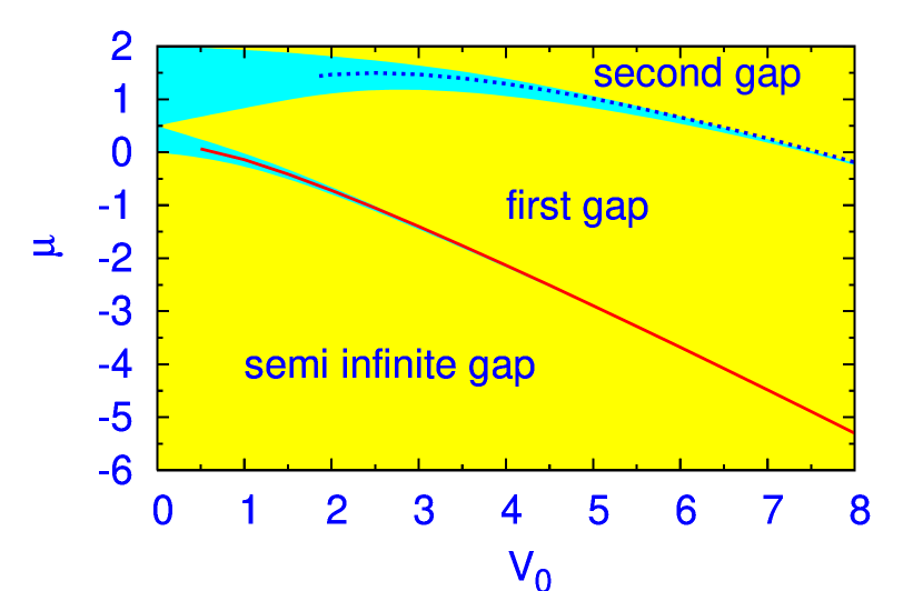
Figure 1: (Color online) The bandgap structure of the linearized version of Eq. (29). Narrow regions between the gaps represent Bloch bands. The solid and dotted curves are borders between the semi-infinite and first finite gaps, and between the first and second finite gaps, as predicted by the variational approximation (see text).

The above-mentioned variational curve shown in Fig. 1 corresponds to a smaller root of Eq. (35). Through the other (larger) root of the same equation, the VA is actually trying to predict another narrow Bloch band, which separates the first and second finite bandgaps in Fig. 1. This root produces a large error in predicting the border between the first and second gaps, as the underlying even ansatz, adopted in Eq. (31), is inadequate in that case. However, the border can be accurately predicted by a modified version of the VA, based on a properly modified (odd) ansatz, see Eq. (48) in Appendix and the dotted blue curve in Fig. 1.

In addition to the VA based on Gaussian ansatz (31), we have also elaborated its counterpart based on the hyperbolic secant, $\phi(x)=\sqrt{M/2W}\mathrm{sech}\left(x/W\right)$. Eventual results produced by this ansatz, which we do not display here, are quite close to those generated by the Gaussian, although the accuracy is slightly lower; in particular, it predicts $\left(\mu_{1}\right)_{\mathrm{left}}^{\mathrm{(var)}}(V_{0}=5)-2.854$, cf. value (37) produced by the Gaussian-based VA.

3.2 Numerical results: fundamental gap solitons

Numerical solutions where obtained by integration of time-dependent Eq. (14) (and time-dependent counterparts of bosonic Eqs. (38), see below), using the Crank-Nicholson discretization scheme, until the solution would converge to a time-independent real form. The equations were discretized using time step $0.0005$ and space step $0.025$, in domain $-20<x<+20$. This method of obtaining the stationary solutions guarantees that they are stable. The results presented here were obtained dropping the small cubic term in Eq. (14); effects induced by this additional term are considered below separately.

The family of fundamental GSs predicted by the VA is characterized by dependence $G_{\mathrm{1D}}^{(7/3)}(\mu)$, which was obtained from a numerical solution of Eqs. (33) and (34) (it can be easily translated into a dependence between $\mu$ and the number of atoms, using Eqs. (16) and (11)). This dependence is displayed for two different values of the OL strength, $V_{0}$, in Fig. 2. For the sake of comparison, the figure includes similar dependences for families of 1D bosonic GSs, as obtained by means of the VA, based on the same ansatz (31), from the following bosonic equations with the cubic and quintic self-repulsive terms,

$$\mu\phi+\frac{1}{2}\phi^{\prime\prime}-\left\{\begin{array}[]{c}G_{\mathrm{1D}}^{(3)}\phi^{3}\\ G_{\mathrm{1D}}^{(5)}\phi^{5}\end{array}\right\}+V_{0}\cos(2x)\phi=0.~{}$$ (38)

Here, wave function $\phi(x)$ is subject to normalization condition (15), and $G_{\mathrm{1D}}^{(3)}=\left(\lambda a_{s}/\pi a_{\mathrm{ho}}^{2}\right)N$ [8, 35], $G_{\mathrm{1D}}^{(5)}=\left(\pi^{2}/2\right)$ $N^{2}$ [23], with $N$ the number of boson atoms, $a_{s}$ the scattering length characterizing the repulsive interactions between them, and $a_{\mathrm{ho}}$ the same transverse-trapping size as above.

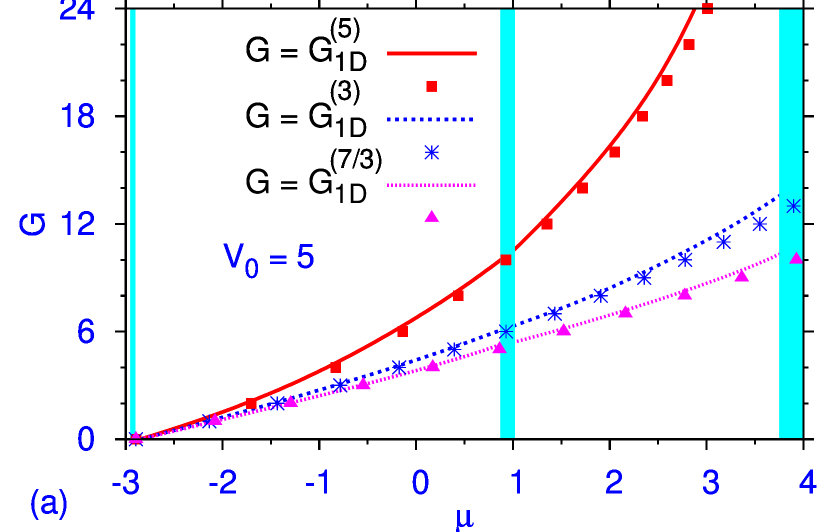
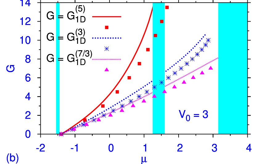
Figure 2: (Color online) The nonlinearity coefficient, $G_{\mathrm{1D}}^{(7/3)}$, in Eq. (14) for the BCS superfluid, versus chemical potential $\mu$, for the family of fundamental 1D gap solitons found in the first two finite bandgaps of periodic potential $-V_{0}\cos(2x)$, with $V_{0}=5$ (a) and $V_{0}=3$ (b). For comparison, also shown are dependences between the respective nonlinear coefficient, $G_{\mathrm{1D}}^{(3)}$ or $G_{\mathrm{1D}}^{(5)}$, and $\mu$ for families of fundamental gap solitons in two 1D bosonic equations (38). Here and in similar figures displayed below, shaded vertical areas represent Bloch bands which separate the gaps. Numerically found solution families are depicted by continuous curves, whereas the predictions produced by the variational approximation are shown by chains of symbols.

Comparison of typical shapes of the numerically found GSs with the respective VA profiles predicted by the Gaussian ansatz is displayed in Fig. 3 (a set of GS shapes obtained from Eq. (38) with the quintic nonlinearity, which is also displayed in this figure, makes it possible to compare the GSs in the BCS superfluid with their bosonic counterparts). The figure includes examples of the GSs belonging to both the first and second bandgaps, which can be easily identified by values of the chemical potential indicated in the panels. In addition to the numerical and variational profiles, in Fig. 3 we also plot their simplest counterparts predicted by the Thomas-Fermi (TF) approximation, which were obtained, as usual [1], by dropping the second-derivative term in Eqs. (29) or (38) (the TF profiles are not shown for very weak nonlinearity, where this approximation is irrelevant)

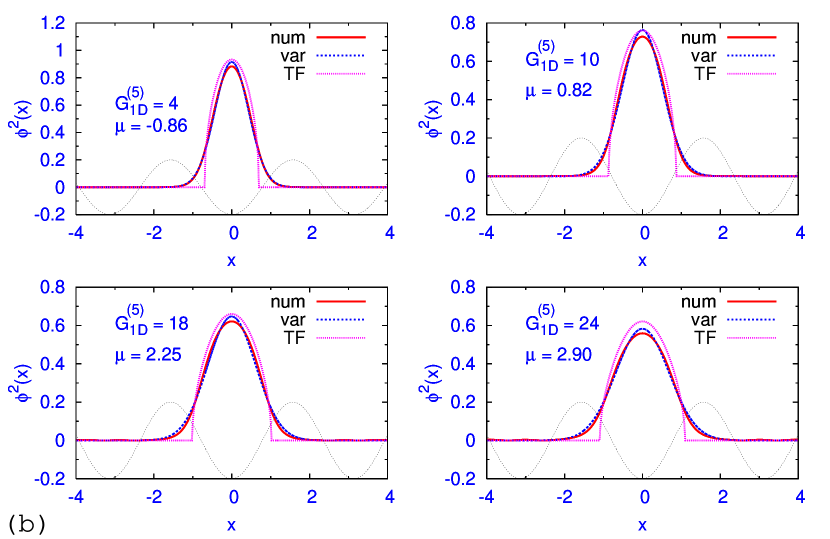
Figure 3: (Color online) One-dimensional GS wave forms (normalized to unity) in the first and second bandgaps as obtained (a) from Eq. (29), without the small cubic term, and (b) from bosonic Eq. (38) with the quintic nonlinearity, for $V_{0}=5$. Here and below, labels “num”, “var”, and “TF” represent numerical, variational, and Thomas-Fermi results, respectively and the thin sinusoidal line depicts the underlying periodic potential, $-V_{0}\cos(2x)$.

Figure 3 demonstrates that the fundamental GSs, unless taken near edges of the bandgaps, are indeed compact objects with a quasi-Gaussian shape, trapped in a single cell of the OL potential. This shape radically changes as one comes very close to a bandgap’s edge, or pushes the solutions to higher values of $\mu$ (in particular, the curves representing the GS family in Eq. (38) with the cubic nonlinearity are aborted in Fig. 2 (b) at a spot where the soliton undergoes a transition to a complex shape with undulating tails, making the further use of the VA irrelevant).

The variational solutions displayed in Fig. 2(a) emerge, at $G=0$, at the value of $\mu$ given by Eq. (37) (recall that it almost exactly coincides with the actual left edge of the first bandgap; the same is true for Fig. 2(b). However, an essential defect of the variational solutions for these families is that they ignore the Bloch band separating the first and second bandgaps, going across it (inside the bands the VA predicts the so-called quasi-solitons, i.e., nearly localized solutions, with the smallest amplitude of nonvanishing tails attached to the central “body” [42]). Another noteworthy inference is that, as seen from Figs. 2 and 3, the accuracy provided by the VA for the description of the GS family generated by Eq. (29) for the BCS superfluid is better than for the bosonic GS families.

3.3 Physical estimates for the fundamental gap solitons

Undoing rescalings (13) and (16), we conclude that conditions (7) and (9), which underlie the derivation of the effective 1D Eq. (14), are definitely satisfied for $G_{\mathrm{1D}}^{(7/3)}>3$, i.e., according to Fig. 2, starting from the middle of the first finite bandgap. To assess the feasibility of the creation of the GSs in the BCS superfluid trapped in the OL, it is necessary to estimate the expected number of atoms, $N$, in the predicted quasi-1D soliton. Getting back to the physical units, we arrive at the following estimates for $N$ and the corresponding value of $n$ (recall it is the largest quantum number of the filled states in the transverse trapping potential, which appears in Eqs. (10) and (11)):

$$N_{\mathrm{1Dsoliton}} \simeq 10^{3}\cdot\left(\frac{m}{m_{\mathrm{eff}}}\right)^{3/2}\left(G_{\mathrm{1D}}^{(7/3)}\right)^{5/2}\left(a_{\mathrm{ho}}/\lambda\right)^{4},$$

$$n^{5} \simeq 10\left(N_{\mathrm{1Dsoliton}}a_{\mathrm{ho}}/\lambda\right)^{2}.$$ (39)

Figure 2 demonstrates that the largest achievable value of the effective nonlinearity strength is $\left(G_{\mathrm{1D}}^{(7/3)}\right)_{\max}\sim 10$. Then, assuming $a_{\mathrm{ho}}/\lambda\sim 1$ (for ⁶Li atoms, this implies the use of trapping frequency $\ \omega_{\perp}\simeq 2\pi\times 1$ KHz, if the OL is induced by light with wavelength $\lambda\simeq 1$ $\mu$m), relations (39) predict $N_{\mathrm{1Dsoliton}}$ in the range of $10^{4}$, with $n\sim 100$. For a larger wavelength, $\lambda\simeq 3$ $\mu$m, one concludes that $N_{\mathrm{1Dsoliton}}$ takes values in the range of $10^{3}$, with $n$ $\sim\allowbreak 20$.

3.4 Bound states of gap solitons

We have also constructed symmetric and antisymmetric (“twisted”) bound states of the fundamental GSs (unlike the SF solutions, considered in Appendix, they are stable solutions to Eq. (14)). These states were formed by placing in-phase or out-of-phase pairs of identical GSs (ones with equal or opposite signs, respectively) in adjacent cells of the OL potential and allowing them to achieve a stable configuration. Typical examples are shown in Fig. 4 (a). In the experiment, the relative phase of adjacent atomic clusters may be controlled by laser beams.

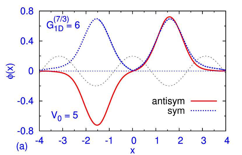
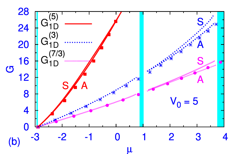
Figure 4: (Color online) (a) Examples of symmetric and antisymmetric (“twisted”) stable bound states of two 1D fundamental GSs, obtained from Eq. (14). (b) Numerically constructed (continuous lines) plots of the nonlinearity versus the chemical potential for symmetric (S) and antisymmetric (A) bound states, for the BCS superfluid and two bosonic models. The analytical results (chains of symbols) are generated using Fig. 2, with $G_{\mathrm{1D}}$ rescaled as described in the text.

The $G_{\mathrm{1D}}(\mu)$ curves for the symmetric and antisymmetric bound states are shown in Fig. 4(b) (again, they are presented together with similar dependences for bound GS pairs generated by two bosonic equations (38)). As might be expected, these curves can be obtained, in an almost exact form, from those for the fundamental solitons (see Fig. 2), by means of rescalings: $G_{\mathrm{1D}}^{(7/3)}\rightarrow 2^{2/3}G_{\mathrm{1D}}^{(7/3)}$, $G_{\mathrm{1D}}^{(3)}\rightarrow 2G_{\mathrm{1D}}^{(3)}$, $G_{\mathrm{1D}}^{(5)}\rightarrow 4G_{\mathrm{1D}}^{(5)}$, respectively. Indeed, if the equations are written in the notation with a fixed nonlinearity coefficient and variable norm, the rescalings simply imply that the norm of the bound state is twice that of the fundamental soliton. The fact that the so defined norm of the symmetric bound states slightly exceeds the norm of their antisymmetric counterparts is natural too, as the vanishing of the density at the center of the antisymmetric state makes its total norm slightly smaller.

3.5 Dragging gap solitons by a moving lattice

A problem of considerable interest is a possibility of controllable transfer of solitons by a moving OL. We have studied this possibility by means of direct simulations of Eqs. (14) and (38), replacing the static OL by $V(x)=-V_{0}\cos\left(2(x+vt)\right)$, which moves at constant velocity $-v$. Typical results for the dragging of GSs taken from the first bandgap are displayed in Fig. 5, both for the bosonic model with the ordinary cubic nonlinearity, and for the model of the BCS superfluid.

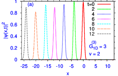
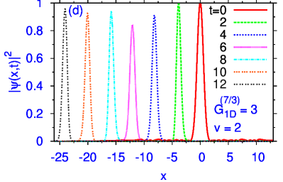
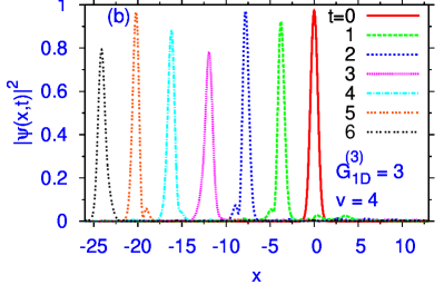
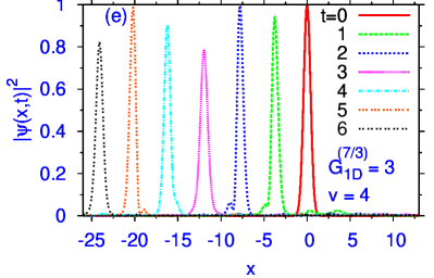
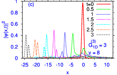
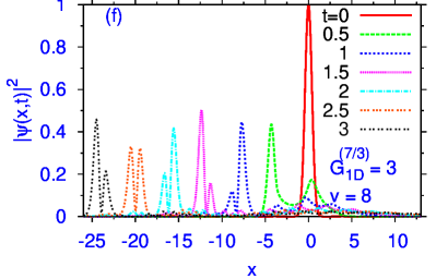
Figure 5: (Color online) Dragging GSs with $G_{\mathrm{1D}}^{(3)}=G_{\mathrm{1D}}^{(7/3)}=3$ by the OL potential $-5\cos[2(x+vt)]$, which was suddenly set in motion at constant velocities $-v=-2,-4,-8$. The upper (BEC) and lower (BCS superfluid) panels display a set of snapshots of the density, taken at consecutive moments of time.

As one might expect, the soliton is dragged in a relatively stable fashion at smaller velocities, but gets destroyed if $v$ is too large. The quality of the transportation may be characterized by the relative loss of the number of atoms in the soliton at the end of the simulation; these data are collected in Table 1 (recall that the initial norm of each soliton is $1$, as per Eq. (15)). It is difficult to exactly identify a critical value of $v$ at which the moving lattice destroys the GS; rather, the transition from the stable dragging (at $v=2$ and $4$) to the destruction (at $v=8$) is gradual. The results for the bosonic model with the quintic nonlinearity (not shown here) are generally similar, although in that case the GS appears to be more fragile, as its destruction commences at velocity $v$ somewhat smaller than in the two models represented in Fig. 5. The above physical estimates suggest that typical length and time units in the present setting are $\sim\,1$ $\mu$m and $1$ ms, from which we infer that the stable transportation of the GSs is possible for velocities $<1$ mm/s.

$v$	$2$	$4$	$8$
BEC	$1.5\%$	$7\%$	$30\%$
BCS superfluid	$2\%$	$8\%$	$28\%$

Table 1. The relative loss of atoms suffered by the one-dimensional gap solitons at the end of dragging shown in Fig. 5.

4 Two-dimensional solitons

4.1 Variational approximation

Stationary solutions to Eq. (18) are looked for as $\psi(x,y,t)=e^{-i\mu t}\phi(x,y)$, with real function $\phi(x)$ obeying equation

$$\mu\phi+(1/2)\left(\partial_{x}^{2}+\partial_{y}^{2}\right)\phi-G_{\mathrm{2D}}^{(7/3)}\phi^{7/3}$$

$$+V_{0}\left[\cos\left(2x\right)+\cos\left(2y\right)\right]\phi=0,$$ (40)

cf. Eq. (29) (the small cubic term is dropped here). Together with normalization condition (20), Eq. (40) can be derived from the respective Lagrangian,

$$L = \int\int dxdy\left\{\mu\phi^{2}-\frac{1}{2}\left(\nabla\phi\right)^{2}-\frac{3}{5}G_{\mathrm{2D}}^{(7/3)}\phi^{10/3}\right.$$ (41)

$$\left.+V_{0}\left[\cos(2x)+\cos(2y)\right]\phi^{2}\right\}-\mu,$$

cf. Eq. (30). To apply the VA, we adopt the 2D Gaussian ansatz, cf. its 1D counterpart (31), as

$$\phi(x,y)=\frac{1}{W}\sqrt{\frac{M}{\pi}}\exp\left(-\frac{x^{2}+y^{2}}{2W^{2}}\right),$$ (42)

where $M$ is the 2D norm, that will be actually fixed as $M=1$, in accordance with Eq. (20) (for the time being, $M$ is one of the variational parameters, together with $\mu$ and width $W$, like in the 1D setting considered above). An anisotropic ansatz for 2D solitons, with different widths in the $x$- and $y$-directions, was considered too. We do not present it here, as numerical solutions of the variational equations have revealed only isotropic solitons.

The substitution of ansatz (42) in Lagrangian (41) yields the effective Lagrangian, cf. Eq. (32)],

$$L_{\mathrm{eff}} = \mu\left(M-1\right)-\frac{M}{2W^{2}}$$ (43)

$$-\frac{9G_{\mathrm{2D}}^{(7/3)}M^{5/3}}{25\pi^{2/3}W^{4/3}}+2V_{0}Me^{-W^{2}}.$$

The first variational equation, $\partial L_{\mathrm{eff}}/\partial\mu=0$, yields, as expected, $M=1$. Then, equations $\partial L_{\mathrm{eff}}/\partial W=\partial L_{\mathrm{eff}}/\partial M=0$ take the following form:

$$\frac{1}{2W^{4}}+\frac{6G_{\mathrm{2D}}^{(7/3)}}{25\pi^{2/3}}\frac{1}{W^{10/3}}=2V_{0}e^{-W^{2}},$$ (44)

$$\mu=\frac{1}{2W^{2}}-2V_{0}e^{-W^{2}}+\frac{3G_{\mathrm{2D}}^{(7/3)}}{5\pi^{2/3}}\frac{1}{W^{4/3}}.$$ (45)

In the linear limit, $G_{\mathrm{2D}}^{(7/3)}=0$, Eq. (44) coincides with its 1D counterpart, Eq. (35). Accordingly, physical solutions ($W^{2}>0$) exist, in the linear limit, for $V_{0}>\left(V_{0}\right)_{\min}=e^{2}/16\approx\allowbreak 0.462$, see Eq. (36). Although the linear Schrödinger equation with a periodic potential cannot have localized solutions (in any dimension), the result obtained in the linear limit makes sense, similar to the situation in the 1D model: after taking $W$ as the smaller root of Eq. (35), and then the respective value of $\mu$ from Eq. (45), one will obtain a value of $\mu$ at which the family of the GS solutions emerges. In this way, the VA predicts the left edge of the first finite bandgap in the 2D spectrum (a similar result was obtained in [41], and for the quasi-1D OL potential in the 2D setting – also in work [43], where the VA could accurately predict the edge of the semi-infinite gap). In particular, the VA gives $\left[\left(\mu_{1}\right)_{\mathrm{left}}^{\mathrm{(var)}}\right]_{\mathrm{2D}}\approx-4.26$ for $V_{0}=4$, whereas the numerical solution of linearized equation (40) yields$\left[\left(\mu_{1}\right)_{\mathrm{left}}^{\mathrm{(num)}}\right]_{\mathrm{2D}}\approx-4.25$ in this case, cf. result (37) and its numerical counterpart, obtained in the 1D case.

4.2 Numerical results

Numerical solutions for 2D solitons were obtained by running simulations of Eq. (18) until the solutions would settle down to stationary real states, as done above for 1D equation (14); recall this procedure produces only stable solutions. The results were compared to the predictions of the VA. For the purpose of the comparison with BEC, we also include findings for the 2D GPE with the usual cubic nonlinearity, whose stationary form is

$$\mu\phi+(1/2)\left(\phi_{xx}+\phi_{yy}\right)-G_{\mathrm{2D}}^{(3)}\phi^{3}$$

$$+V_{0}\left[\cos(2x)+\cos(2y)\right]\phi=0,~{}$$ (46)

cf. one-dimensional equation (38). Solutions to this equation are normalized as in Eq. (20), hence the respective nonlinearity coefficient is [35] $G_{\mathrm{2D}}^{(3)}=2\sqrt{2\pi}\left(a_{s}/a_{\mathrm{ho}}\right)N$, where $a_{\mathrm{ho}}$ characterizes the tight confinement in direction $z$.

Typical examples of the 2D GSs belonging to the first and second bandgaps of the 2D spectrum, which are displayed in Fig. 6 (and many other examples not shown here) demonstrate that the VA provides a good fit to the numerically found shapes, although, of course, simple Gaussian ansatz (42) does not capture very weak tails attached to the central body of the solitons, that become (barely) visible in 2D numerical solutions taken near the edge of the bandgap. In the bosonic model with the cubic nonlinearity, the variational and numerically found soliton shapes are very close too (not shown here).

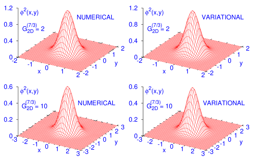
Figure 6: (Color online) Examples of stable 2D GSs, obtained in the numerical and variational forms from Eq. (18) for $V_{0}=4$. The smaller and larger values of $G_{\mathrm{2D}}$ correspond to the first and second bandgaps, respectively, see Fig. 7.

To quantify the accuracy provided by the VA, we calculated the corresponding relative error,

$$\mathrm{err}=\frac{\int\int dxdy\left||\phi_{\mathrm{num}}(x,y)|^{2}-|\phi_{\mathrm{var}}(x,y)|^{2}\right|}{\int\int dxdy|\phi_{\mathrm{num}}(x,y)|^{2}}.$$

For $G_{\mathrm{2D}}^{7/3}=2$ and $G_{\mathrm{2D}}^{7/3}=10$, which are the cases displayed in Fig. 6, we have found $\mathrm{err}=0.020$, and $0.079$, respectively, which illustrates the accuracy provided by the VA for 2D solitons. With the increase of nonlinearity, the shape of the soliton slightly deviates from the Gaussian, which gives rise to a larger value of error.

In addition to Eq. (18) with the square-shaped OL, we have also considered the same equation with the radial-lattice potential (the small cubic term is dropped here),

$$i\psi_{t}=-\frac{1}{2}\nabla^{2}\psi-G_{\mathrm{2D}}^{(7/3)}|\psi|^{4/3}\psi+V_{0}\cos\left(2r\right)\psi=0.$$ (47)

Unlike previously studied 2D models with the repulsive cubic nonlinearity and radial potential of the Bessel type [44], the potential in Eq. (47) does not vanish at $r\rightarrow\infty$, hence radial GSs can be produced by this equation [32]. The shape of these solitons (not shown here) is quite similar to that of the GSs supported, at the same values of $G_{\mathrm{2D}}^{(7/3)}$, by the square lattice, which suggests that the square OL gives rise to nearly isotropic solitons.

Bearing in mind normalization condition (20), families of fundamental two-dimensional GSs are characterized by dependence $G_{\mathrm{2D}}^{(7/3)}(\mu)$ (and its counterpart, $G_{\mathrm{2D}}^{(3)}(\mu)$, for bosonic Eq. (46)), similar to the 1D model. These dependences, as predicted by the VA and found from the numerical solutions, are displayed in Fig. 7 (the VA for Eq. (46) was also based on ansatz (42)). Numerical results for the family of the radial GSs obtained from Eq. (47) are included too.

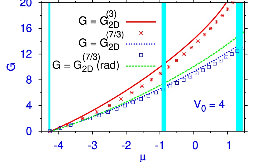
Figure 7: (Color online) The numerical (continuous lines) and variational (strings of symbols) nonlinearity-versus-chemical-potential plots for 2D GSs obtained from Eqs. (18) and (46). The curve labeled “$G=G_{\mathrm{3D}}^{(7/3)}$(rad)” additionally displays numerical results for radial GSs generated by Eq. (47) with the axisymmetric potential.

A conclusion is that the VA provides good accuracy in describing the GS families in both models with the square-lattice potential, although, as in the 1D case, the approximation formally predicts that the families continue across the narrow Bloch band separating the first and second bandgaps, where solitons cannot exist. Another noteworthy similarity to the 1D case is that the VA yields a higher accuracy for  the nonlinearity of power $7/3$ than for its cubic counterpart.

The family of 2D GSs was also constructed taking into regard the additional cubic term in Eq. (18). It was found that, as well as in the 1D case, this term, if taken with physically relevant values of the coefficient in front of it (an estimate for which is given below), produced a negligible effect.

4.3 Physical estimates for the two-dimensional solitons

As said above, underlying conditions (7) and (9) definitely hold for the 2D GSs generated by Eq. (18). Proceeding to the estimate for the number of atoms in 2D solitons in the BCS superfluid, it is relevant to mention that no two- (or three-) dimensional matter-wave solitons of any type, regular or gap-mode, have been created, thus far, even in BEC, therefore exploring new possibilities for the creation of multidimensional matter-wave solitons may be quite relevant to the experiment.

Figure 7 demonstrates that achievable values of the normalized nonlinearity strength for 2D GSs are $\left(G_{\mathrm{2D}}^{(7/3)}\right)_{\max}\simeq 15$. Undoing rescalings (17) and (19), we conclude that the corresponding number of atoms in the soliton is in the range of $\left(N_{\mathrm{2Dsoliton}}\right)_{\max}\sim 10^{3}$, the respective largest quantum number of the filled states in the transverse trapping potential being $n\sim 10$. This number of atoms is sufficient to justify the consideration of solitons in terms of the BCS superfluid, and to make experimental observation of the solitons possible.

As for the coefficient in front of the additional cubic term in Eq. (18), the estimate making use of expression (19) demonstrates that it may achieve values $\left|g_{\mathrm{2D}}\right|\sim 0.1$, which are higher than $\left|g_{\mathrm{1D}}\right|\sim 10^{-3}$ in the 1D geometry (see above), but still quite small in comparison with $G_{\mathrm{2D}}^{(7/3)}$.

5 Conclusion

The objective of this work was to predict the existence of quasi-1D and quasi-2D solitons in the BCS superfluid formed by a gas of fermion atoms, with weak attraction between atoms with opposite orientations of their spins. We considered the experimentally relevant configuration of the gas trapped under the combined action of the 1D or 2D optical lattice (OL) and tight 2D or 1D trap applied in the transverse direction(s). The analysis was based on the 3D equation for the wave function derived from the Lagrangian that included the energy density of the weakly coupled BCS superfluid. Then, the equation was reduced to effective 1D and 2D equations, taking into regard the tight transverse confinement. A characteristic feature of the equations is the self-repulsive nonlinear term of power $7/3$; it was also shown that the next-order correction to the energy density of the weakly coupled superfluid gives rise to a small additional cubic term in the equations. Families of stable one- and two-dimensional GSs (gap solitons) were found, by means of the VA (variational approximation) and in the numerical form, in the first two finite bandgaps of the OL-induced spectrum. The VA, based on the Gaussian ansatz, provides good accuracy in the description of the families of 1D and 2D solitons, except for very close to edges of the bandgaps, where the GS changes its shape from tightly- to a loosely-bound one, with undulating tails. In the linear limit, the VA accurately predicts borders (i.e., narrow Bloch bands) separating different gaps in the spectrum. The comparison with the predictions for 1D and 2D bosonic GSs, supported by the cubic (or quintic) repulsive nonlinearity, has demonstrated that the VA provides a higher accuracy in predicting the solitons in the present model with the weaker nonlinearity, of power $7/3$. Even and odd stable bound states of one-dimensional GSs were found too. They may be interpreted as pairs of fundamental solitons placed in adjacent local wells of the lattice. In the 2D case, additionally found solutions are radial GSs supported by the radial-lattice potential.

The quasi-1D and quasi-2D gap solitons, confined by the moderately strong transverse potential, may contain the number of fermion atoms in the ranges of $10^{3}-10^{4}$ and $10^{3}$, respectively. The possibility of dragging GSs by a moving OL was studied in the 1D setting. It was demonstrated that there is a smooth transition from a regime of stable motion of the soliton to its destruction, as the OL’s velocity increases beyond $\sim 1$ mm/s.

Experimental creation of the quasi-1D and quasi-2D gap solitons in the BCS superfluid seems quite feasible. As concerns further developments of the theory, issues of straightforward interest are 3D solitons, as well as vortex solitons in two dimensions.

We appreciate valuable discussions with L. Salasnich. The work of S.K.A. was supported in a part by FAPESP and CNPq (Brazil). The work of B.A.M. was partly supported by the Israel Science Foundation through the Center-of-Excellence grant No. 8006/03, and by the German-Israel Foundation through Grant No. 149/2006. B.A.M. appreciates hospitality of the Institute of Theoretical Physics at UNESP (São Paulo State University) and financial assistance from FAPESP.

Appendix: one-dimensional subfundamental solitons

The ordinary one-dimensional GPE with the repulsive cubic nonlinearity and OL potential, which corresponds to the first line in Eq. (38), gives rise to antisymmetric SF (subfundamental) solitons, which were found in the second bandgap of the OL-induced spectrum in work [45]. They are called so because, if one uses the notation with fixed $G_{\mathrm{3D}}^{(3)}$ and arbitrary norm, these solitons have the norm which is lower than in the fundamental bosonic GSs, for the same chemical potential. A characteristic feature of the SF solitons is that two maxima of the density, $|\phi(x)|^{2}$, are located inside a single cell of the OL potential (i.e., this antisymmetric soliton as a whole is essentially confined to the single cell). The SF solitons are different from antisymmetric bound states of two fundamental solitons, which feature two maxima of $\left|\phi(x)\right|^{2}$ located in different potential wells, see Fig. 4(a).

In the 1D model derived in this work, i.e., Eq. (14), families of SF solitons can also be found in the second bandgap. They are unstable, although their instability is weak, as, otherwise, the numerical method described above, which is based on the direct integration of Eq. (14), would not reveal them. Similar to the situation in the GPE, the instability does not completely destroy the SF solitons, but rather converts them into fundamental GSs belonging to the first finite bandgap.

The SF solitons, as odd solutions to Eq. (29), may be represented by the VA based on the accordingly modified Gaussian ansatz,

$$\phi(x)=\pi^{-1/4}\frac{\sqrt{2M}}{W^{3/2}}x\exp\left(-\frac{x^{2}}{2W^{2}}\right)$$ (48)

(its norm is $1$ for $M=1$). Inserting this ansatz in Lagrangian (30) yields

$$L = \mu\left(M-1\right)-\frac{3M}{4W^{2}}+{V}_{0}M(1-2W^{2})e^{-W^{2}}$$ (49)

$$- \frac{2^{5/3}\Gamma\left(13/6\right)}{\left(5/3\right)^{19/6}\pi^{5/6}}G_{\mathrm{1D}}^{(7/3)}\frac{M^{5/3}}{W^{2/3}}~{},$$

cf. Eq. (32). The first variational equation following from Eq. (49), $\partial L/\partial\mu=0$, gives $M=1$, as before. The remaining equations, $\partial L/\partial W=0$ and $\partial L/\partial M=0$, take the following form, cf. Eqs. (33) and (34):

$$1 + \frac{2^{11/3}\Gamma\left(13/6\right)}{9\left(5/3\right)^{19/6}\pi^{5/6}}G_{\mathrm{1D}}^{(7/3)}W^{4/3}$$ (50)

$$= \frac{4}{3}V_{0}W^{4}(3-2W^{2})e^{-W^{2}},$$

$$\mu = \frac{3}{4W^{2}}+\frac{2^{5/3}\Gamma(13/6)}{\left(5/3\right)^{13/6}\pi^{5/6}}\frac{G_{\mathrm{1D}}^{(7/3)}}{W^{2/3}}$$ (51)

$$- {V_{0}}(1-2W^{2})e^{-W^{2}}.$$

Note that setting $G_{\mathrm{1D}}^{(7/3)}=0$ in Eq. (50) yields an equation for $W^{2}$ which has two physical roots if $V_{0}$ exceeds a minimum value, $\left(V_{0}\right)_{\min}\approx 0.37$, cf. expression (36) for the minimum value of $V_{0}$ in the VA based on ansatz (31). The smaller root, if substituted in Eq. (51) with $G_{\mathrm{1D}}^{(7/3)}=0$, yields $\left(\mu_{2}\right)_{\mathrm{left}}^{\mathrm{(var)}}\equiv\mu\left(G_{\mathrm{1D}}^{(7/3)}=0\right)$, which, as shown by the dotted curve in Fig. 1, accurately predicts the lower/left edge of the second bandgap. In particular, this approximation predicts $\left(\mu_{1}\right)_{\mathrm{left}}^{\mathrm{(var)}}\approx 1.02$ for $V_{0}=5$, while the respective value obtained from the numerical solution of the Mathieu equation is $\mu_{12}^{\mathrm{(num)}}(V_{0}=5)\approx 1.03$, cf. variational prediction (37) for the border between the semi-infinite and first finite gaps.

The comparison of the dependence $G_{\mathrm{1D}}^{(7/3)}(\mu)$ for the SF solitons in the second bandgap, as predicted by Eqs. (50) and (51), versus its numerically found counterpart is presented in Fig. 8(a). Again, for the purpose of comparison, this figure additionally includes dependences between the nonlinearity strength and chemical potential of SF solitons, as obtained in the numerical form and by means of the VA (that was also based on ansatz (48)) for two bosonic equations (38). As seen from this figure and Fig. 2, the accuracy of the variational prediction for the SF soliton families is worse than it was for the fundamental GSs. Nevertheless, the prediction is still acceptable for the SF solitons in the BCS-superfluid model. In particular, the shape of the SF solitons in this model is approximated by the VA quite accurately, as shown in Fig. 8(b). On the other hand, it is evident from Fig. 8(a) that the discrepancy between the VA and numerical results for the SF solitons found in the bosonic models is much larger, which strongly confirms the above inference that the VA works essentially better in the model of the BCS superfluid than in the BEC models, i.e., for the nonlinearity of power $7/3$ than for the cubic and quintic nonlinear terms.

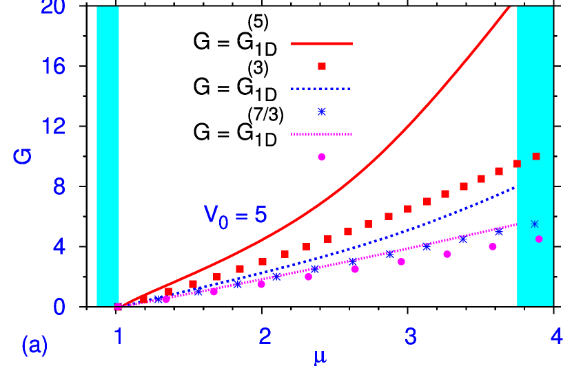
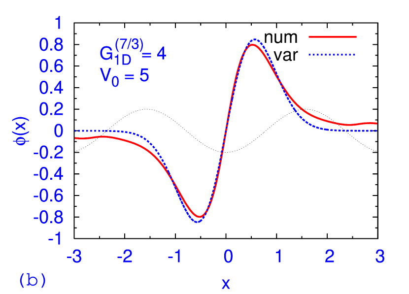
Figure 8: (Color online) (a) The same as in Fig. 2, but for 1D subfundamental solitons, found in the second finite bandgap. (b) A typical example of the subfundamental soliton found from the numerical solution of Eq. (29), and its variational counterpart.

References

- [1] C. Pethick, H. Smith. Bose-Einstein Condensation in Dilute Gases (Cambridge University Press: Cambridge, 2002); L. P. Pitaevskii, S. Stringari. Bose-Einstein Condensation (Clarendon Press: Oxford and New York, 2003).
- [2] A. Minguzzi, S. Succi, F. Toschi, M. P. Tosi, P. Vignolo, Phys. Rep. 395 (2004) 223; Q. J. Chen, J. Stajic, S. Tan, K. Levin, Phys. Rep. 412 (2005) 1.
- [3] K. E. Strecker, G. B. Partridge, A. G. Truscott, R. G. Hulet, New J. Phys. 5 (2003) 73; V. A. Brazhnyi, V. V. Konotop, Mod. Phys. Lett. B 18 (2004) 627; F. Kh. Abdullaev, A. Gammal, A. M. Kamchatnov, L. Tomio, Int. J. Mod. Phys. B 19 (2005) 3415; F. Dalfovo, S. Giorgini, L. P. Pitaevskii, S. Stringari, Rev. Mod. Phys. 71 (1999) 463; V. I. Yukalov, Laser Phys. Lett. 1 (2004) 435.
- [4] K. E. Strecker, G. B. Partridge, A. G. Truscott, R. G. Hulet, Nature 417 (2002) 150; L. Khaykovich, F. Schreck, G. Ferrari, T. Bourdel, J. Cubizolles, L. D. Carr, Y. Castin, C. Salomon, Science 256 (2002) 1290; V. M. Pérez-García, H. Michinel, H. Herrero, Phys. Rev. A 57 (1998) 3837.
- [5] S. L. Cornish, S. T. Thompson, C. E. Wieman, Phys. Rev. Lett. 96 (2006) 170401.
- [6] S. Inouye, M. R. Andrews, J. Stenger, H. J. Miesner, D. M. Stamper-Kurn, W. Ketterle, Nature 392 (1998) 151.
- [7] M. Zaccanti, C. D’Errico, F. Ferlaino, G. Roati, M. Inguscio, G. Modugno, Phys. Rev. A 74 (2006) 041605(R); S. Ospelkaus, C. Ospelkaus, L. Humbert, K. Sengstock, K. Bongs, Phys. Rev. Lett. 97 (2006) 120403.
- [8] G. L. Alfimov, V. V. Konotop, M. Salerno, Europhys. Lett. 58 (2002) 7; B. B. Baizakov, V. V. Konotop, M. Salerno, J. Phys. B 35 (2002) 51015; P. J. Y. Louis, E. A. Ostrovskaya, C. M. Savage, Y. S. Kivshar, Phys. Rev. A 67 (2003) 013602
- [9] H. Sakaguchi, B. A. Malomed, J. Phys. B 37 (2004) 1443; H. Sakaguchi, B. A. Malomed, J. Phys. B 37 (2004) 2225.
- [10] K. M. Hilligsøe, M. K. Oberthaler, K.-P. Marzlin, Phys. Rev. A 66 (2002) 063605; D. E. Pelinovsky, A. A. Sukhorukov, Y. S. Kivshar, Phys. Rev. E 70 (2004) 036618.
- [11] B. Eiermann, Th. Anker, M. Albiez, M. Taglieber, P. Treutlein, K.-P. Marzlin, M. K. Oberthaler, Phys. Rev. Lett. 92 (2004) 230401.
- [12] O. Morsch, M. Oberthaler, Rev. Mod. Phys. 78 (2006) 179.
- [13] V. Ahufinger, A. Sanpera, P. Pedri, L. Santos, M. Lewenstein, Phys. Rev. A 69 (2004) 053604.
- [14] M. Matuszewski, W. Królikowski, M. Trippenbach, Y. S. Kivshar, Phys. Rev. A 73 (2006) 063621.
- [15] B. DeMarco, D. S. Jin, Science 285 (1999) 1703; C. A. Regal, D. S. Jin, Adv. At. Mol. Opt. Phys. 54 (2007) 1.
- [16] T. Karpiuk, K. Brewczyk, S. Ospelkaus-Schwarzer, K. Bongs, M. Gajda, K. Rzazewski, Phys. Rev. Lett. 93 (2004) 100401; T. Karpiuk, M. Brewczyk, K. Rzazewski, Phys. Rev. A 73 (2006) 053602.
- [17] S. K. Adhikari, Phys. Rev. A 72 (2005) 053608.
- [18] A. Gubeskys, B. A. Malomed, I. M. Merhasin, Phys. Rev. A 73 (2006) 023607.
- [19] V. M. Pérez-García, J. B. Beitia, Phys. Rev. A 72 (2005) 033620; S. K. Adhikari, Phys. Lett. A 346 (2005) 179; T. C. Lin, J. C. Wei, Nonlinearity 19 (2006) 2755; S. K. Adhikari, B. A. Malomed, Phys. Rev. 77 (2008) 023607.
- [20] V. Yu. Bludov, J. Santhanam, V. M. Kenkre, V. V. Konotop, Phys. Rev. A 74 (2006) 043620.
- [21] S. K. Adhikari, L. Salasnich, Phys. Rev. A 76 (2007) 023612.
- [22] L. Tonks, Phys. Rev. 50 (1936) 955; M. Girardeau, J. Math. Phys. 1 (1960) 516; M. D. Girardeau, Phys. Rev. 139 (1965) B500.
- [23] E. B. Kolomeisky, T. J. Newman, J. P. Straley, X. Qi, Phys. Rev. Lett. 85 (2000) 1146; E. H. Lieb, R. Seiringer, J. Yngvason, Phys. Rev. Lett. 91 (2003) 150401; B. Damski, J. Phys. B 37 (2004) L85; J. Brand, J. Phys. B 37 (2004) S287; G. E. Astrakharchik, D. Blume, S. Giorgini, L. P. Pitaevskii, Phys. Rev. Lett. 93 (2004) 050402; G. E. Astrakharchik, D. Blume, S. Giorgini, B. E. Granger, J. Phys. B 37 (2004) S205.
- [24] F. Kh. Abdullaev, M. Salerno, Phys. Rev. A 72 (2005) 033617; G. L. Alfimov, V. V. Konotop, P. Pacciani, Phys. Rev. A 75 (2007) 023624.
- [25] M. Salerno, Phys. Rev. A 72 (2005) 063602.
- [26] J. R. Schrieffer, Theory of Superconductivity, W. A. Benjamin, Reading, 1964; M. Tinkham, Introduction to Superconductivity, 2nd Ed., McGraw Hill, New York, 1996.
- [27] S. K. Adhikari, B. A. Malomed, Europhys. Lett. 79 (2007) 50003.
- [28] K. Huang, C. N. Yang, Phys. Rev 105 (1957) 767; T. D. Lee, C. N. Yang, Phys. Rev. 105 (1957) 1119.
- [29] V. M. Pérez-García, H. Michinel, J. I. Cirac, M. Lewenstein, P. Zoller, Phys. Rev. A 56 (1997) 1424.
- [30] S. K. Adhikari, B. A. Malomed, Phys. Rev. A 76 (2007) 043626.
- [31] G. Theocharis, D. J. Frantzeskakis, R. Carretero-González, P. G. Kevrekidis, B. A. Malomed, Phys. Rev E 71 (2005) 017602; P. G. Kevrekidis, D. J. Frantzeskakis, R. Carretero-González, B. A. Malomed, G. Herring, A, Bishop, Phys. Rev A 71 (2005) 023614.
- [32] B. B. Baizakov, B. A. Malomed, and M. Salerno, Phys. Rev. E 74 (2006) 066615.
- [33] N. Manini, L. Salasnich,Phys. Rev A 71 (2005) 033625.
- [34] S. K. Adhikari, Phys. Rev. A 76 (2007) 053609; S. K. Adhikari, Phys. Rev. A 77 (2008) 045602; S. K. Adhikari, Eur. Phys. J. D 47 (2008) 413; A. Bulgac, Phys. Rev. A 76 (2007) 050402(R).
- [35] L. Salasnich, Laser Phys. 12 (2002) 198; L. Salasnich, A. Parola, L. Reatto, J. Phys. B 39 (2006) 2839; L. Salasnich, B. A. Malomed, Phys. Rev. A 74 (2006) 053610.
- [36] A. E. Muryshev, G. V. Shlyapnikov, W. Ertmer, K. Sengstock, M. Lewenstein, Phys. Rev. Lett. 89 (2002) 110401; L. Khaykovich, B. A. Malomed, Phys. Rev. A 74 (2006) 023607.
- [37] Y. B. Band, I. Towers, B. A. Malomed, Phys. Rev. A 67 (2003) 023602; S. De Nicola, B. A. Malomed, R. Fedele, Phys. Lett. A 360 (2006) 164.
- [38] C. N. Yang, Phys. Rev. Lett 19 (1967) 1312; M. Gaudin, Phys. Lett. A 24 (1967) 55.
- [39] I. V. Tokatly, Phys. Rev. Lett 93 (2004) 090405.
- [40] L. Salasnich, Phys. Rev A 76 (2007) 015601.
- [41] A. Gubeskys, B. A. Malomed, I. Merhasin, Stud. Appl. Math. 115 (2005) 255.
- [42] D. J. Kaup and B. A. Malomed, J. Opt. Soc. Am. B 15 (1998) 2838; Physica D 184 (2003) 153.
- [43] T. Mayteevarunyoo, B. A. Malomed, and M. Krairiksh, Phys. Rev. A 76, 053612 (2007).
- [44] Y. V. Kartashov, V. A. Vysloukh, L. Torner, Phys. Rev. Lett. 94 (2005) 043902; Y. V. Kartashov, R. Carretero-González, B. A. Malomed, V. A. Vysloukh, L. Torner.Opt. Exp. 13 (2005) 10703.
- [45] T. Mayteevarunyoo and B. A. Malomed, Phys. Rev. A 74 (2006) 033616.