Frequency locking in the injection-locked frequency divider equation

Abstract

We consider a model for the injection-locked frequency divider, and study analytically the locking onto rational multiples of the driving frequency. We provide explicit formulae for the width of the plateaux appearing in the devil’s staircase structure of the lockings, and in particular show that the largest plateaux correspond to even integer values for the ratio of the frequency of the driving signal to the frequency of the output signal. Our results prove the experimental and numerical results available in the literature.

1 Introduction

In [28], an electronic circuit known as the injection-locked frequency divider is studied experimentally, and the devil’s staircase structure of the lockings is measured: when the ratio of the frequency $\omega$ of the driving signal to the frequency $\Omega$ of the output signal is plotted versus $\omega$, plateaux are found for rational values of the ratio. In [29], a model for the circuit is presented and numerically investigated, and the results are shown to agree with the experiments.

In this paper, on the basis of the model introduced in [29], we address the problem of explaining analytically the appearance of the plateaux of the devil’s staircase. We aim to understand why the largest plateaux correspond to even integer values for the frequency ratio and, more generally, how the widths of the plateaux depend on the particular values of the ratio.

From a qualitative point of view, the mechanism of locking can be illustrated as follows. For fixed driving frequency $\omega$ one considers the Poincaré section at times $t=2\pi n/\omega$, for integer $n$, and studies the dynamics on the attractor. This leads to a map which behaves as a diffeomorphism on the circle. Thus, based on the theory of such systems [3], one expects that for $\omega/\Omega_{0}$ close to a rational number one has locking. How close $\omega$ has to be to a rational multiple of $\Omega_{0}$ depends on $\mu$ and on the multiple itself: in the $(\omega,\mu)$ parameter plane one has locking in wedge-shaped regions known as Arnold tongues.

However, all the discussion above is purely qualitative. In particular, there remains the major problem of determining the map to which one should apply the theory. A quantitative constructive analysis is another matter, and requires taking into account the fine details of the equation and the explicit expression of the solution of the unperturbed equation: we carry this out in this paper. Our analysis is based on perturbation theory, which is implemented to all orders and proved to be convergent. This approach is particularly suited for quantitative estimates within any given accuracy (for which it has to be possible to go to arbitrarily high perturbation orders, and to control the truncation errors). Furthermore, we think that a rigorous analysis ab initio, without introducing uncontrolled simplifications or approximations, can be of interest by itself. Indeed, although such simplifications can capture the essential features of the problem and allow a qualitative understanding of the physical phenomenon, it nonetheless remains unclear in general how far a simplified model can be expected to describe the original system faithfully.

The conclusions of our analysis can be summarised as follows. The equation modelling the system can be viewed as a perturbation of order $\mu$ of a particular differential equation. In the absence of the perturbation, after a suitable change of variables, the system can be cast in the form of a Liénard equation $x^{\prime\prime}+h(x)\,x^{\prime}+k(x)=0$. Under suitable assumptions on $h$ and $k$, this admits a globally attracting limit cycle. Let $\Omega_{0}$ be the proper frequency of such a cycle, and let us denote by $x_{0}(t)=X_{0}(\Omega_{0}t)$ the solution of the equation corresponding to the limit cycle, with the function $X_{0}$ being $2\pi$-periodic in its argument. By also including the time direction, one can study the dynamics in the three-dimensional extended phase space $(x,x^{\prime},t)$, in which the limit cycle generates a topological cylinder. When the perturbation is switched on, the cylinder survives as an invariant manifold, slightly deformed with respect to the unperturbed case. This follows from general arguments related to the centre manifold theorem [9]. However the dynamics on the manifold strongly depends on the relation between the proper frequency $\Omega_{0}$ and the frequency $\omega$ of the driving signal. If $\omega/\Omega_{0}$ is irrational and satisfies some Diophantine condition (such as $|\omega\nu_{1}+\Omega_{0}\nu_{2}|>\gamma(|\nu_{1}|+|\nu_{2}|+1)^{-\tau}$ for all $(\nu_{1},\nu_{2})\in\mathds{Z}^{2}$ and some positive constants $\gamma,\tau$), then one expects the output signal $x(t)$ to be a quasi-periodic function with frequency vector $\boldsymbol{\omega}=(\omega,\Omega_{0})$, so that one has $x(t)=X(\omega t,\Omega_{0}t)=X_{0}(\Omega_{0}t)+O(\mu)$, where $X$ is a $2\pi$-periodic function of both its arguments. In this case we say that the output frequency $\Omega$ equals $\Omega_{0}$ (of course, this is slightly improper terminology because $\Omega_{0}$ is only the frequency of the leading contribution to the output signal, and the latter is not even periodic). On the other hand, if $\omega/\Omega_{0}$ is close to a rational number $p/q$ (resonance), then $x(t)$ is periodic with frequency $\Omega=p\omega/q$ (locking): hence the frequency $\Omega$ of the output signal differs from $\Omega_{0}$ — even if it remains close to it —, because it is locked to the driving frequency $\omega$. Thus, if one plots the ratio $\omega/\Omega$ versus $\omega$ one obtains the devil’s staircase structure depicted in Figures 4 to 9 of [28]. The locked solutions can be obtained analytically from the unperturbed periodic solutions by a mechanism similar to the subharmonic bifurcations that we have studied in previous papers [4, 6]. We stress, however, that, unlike the cases studied in the latter references, here, the unperturbed equation cannot be solved in closed form. This will yield extra technical difficulties, because we shall have to rely for our analysis on abstract symmetry properties of the solution, without the possibility of using explicit expressions.

2 Model for the injection-locked frequency divider

We consider the system of ordinary differential equations

$$C\frac{{\rm d}V_{C}}{{\rm d}t}=I_{L}+f(V_{C},t),\qquad L\frac{{\rm d}I_{L}}{{\rm d}t}=-RI_{L}-V_{C},$$ (2.1)

where $L,C,R>0$ are parameters, $V_{C}$ and $I_{L}$, the state variables, are the capacitor voltage and the inductor current, respectively, and

$$f(V_{C},t)=\left(A+B\sin\Omega t\right)V_{C}\left(1-\left(V_{C}/V_{DD}\right)^{2}\right),\qquad V_{DD},A>0,\qquad B\in\mathds{R},$$

is the (cubic approximation of the) driving point characteristic of the nonlinear resistor. The model (2.1) was introduced in [29] as a simplified description of the injection-locked frequency divider.

By introducing the new variables $u:=V_{C}/V_{DD}$ and $v:=RI_{L}/V_{DD}$ and rescaling time $t\to Rt/L$, (2.1) becomes

$$u^{\prime}=\alpha v+\Phi(t)\,u\left(1-u^{2}\right),\qquad v^{\prime}=-u-v,$$ (2.2)

where the prime denotes derivative with respect to time $t$, and we have set $\alpha=L/R^{2}C$, $\beta=LA/RC$, $\mu=LB/RC$, and $\Phi(t)=\beta+\mu\sin\omega t$, with $\omega=\Omega L/R$.

From now on, we shall consider the system (2.2), with $\alpha>\beta>1$, and $\mu,\omega\in\mathds{R}$. By setting $\sigma=u+v$ we obtain

$$\sigma^{\prime}=\left(\alpha-1\right)\sigma+\left(\Phi(t)-\alpha\right)u-\Phi(t)\,u^{3},\qquad u^{\prime}=\alpha\,\sigma+\left(\Phi(t)-\alpha\right)u-\Phi(t)\,u^{3},$$ (2.3)

which gives $u^{\prime\prime}+\left[1-\Phi(t)+3\Phi(t)u^{2}\right]u^{\prime}+\left[\left(\alpha-\Phi(t)\right)u+\Phi(t)\,u^{3}\right]+\Phi^{\prime}(t)\left(u^{3}-u\right)=0$, that is

$$u^{\prime\prime}+\left(1-\beta+3\beta u^{2}\right)u^{\prime}+\left[\left(\alpha-\beta\right)u+\beta\,u^{3}\right]+\mu\Psi(u,u^{\prime},t)=0,$$ (2.4)

with

$$\Psi(u,u^{\prime},t)=\left[u^{\prime}\left(3u^{2}-1\right)\sin\omega t+\left(u^{3}-u\right)\sin\omega t+\omega\left(u^{3}-u\right)\cos\omega t\right].$$ (2.5)

For $\mu=0$, (2.4) reduces to $u^{\prime\prime}+(1-\beta+3\beta u^{2})\,u^{\prime}+[(\alpha-\beta)\,u+\beta\,u^{3}]=0$, which can be written as a Liénard equation

$$u^{\prime\prime}+u^{\prime}\,h(u)+k(u)=0,$$ (2.6)

with

$$h(u)=1-\beta+3\beta u^{2},\qquad k(u)=\left(\alpha-\beta\right)u+\beta u^{3}=u\left(\alpha-\beta+\beta u^{2}\right).$$ (2.7)

For (2.6) to have a unique limit cycle [10, 20], we require that

$$1-\beta<0,\qquad\alpha-\beta>0\qquad\Longrightarrow\qquad\alpha>\beta>1,$$

which motivates our assumptions on the parameters $\alpha$ and $\beta$.

Consider the system described by the equation (2.6), with the functions $h(u)$ and $k(u)$ given by (2.7) with $\alpha>\beta>1$. Such a system admits one and only one limit cycle encircling the origin [20]; cf. Figure 1. Let $T_{0}$ be the period of the solution $u_{0}(t)$ running on such a cycle. Denote by $\Omega_{0}=2\pi/T_{0}$ the corresponding frequency: $\Omega_{0}$ will be called the proper frequency of the system. Note that $\Omega_{0}$ depends only on the parameters $\alpha$ and $\beta$.

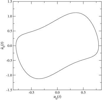
Figure 1: The limit cycle for $\alpha=2.5$, $\beta=2.0$ and $\mu=0$. The proper frequency is $\Omega_{0}\approx 1.1434$.

The solution $u_{0}(t)$ is unique up to time translation. Fix the time origin so that $u^{\prime}_{0}(0)=0$, $u_{0}(0)>0$. Note that fixing the origin of time in such a way that $u^{\prime}_{0}(0)=0$ compels us to shift by some $t_{0}$ the time in the argument of the driving term in (2.5), i.e. $\Psi(u,u^{\prime},t)$ must be replaced with $\Psi(u,u^{\prime},t+t_{0})$; cf. the analogous discussion in [17].

Lemma 1

The Fourier expansion of $u_{0}(t)$ contains only the odd harmonics, i.e.

$$u_{0}(t)=\sum_{\nu\in\mathds{Z}}{\rm e}^{i\Omega_{0}\nu t}u_{0,\nu}=\sum_{\begin{subarray}{c}\nu\in\mathds{Z}\\ \nu\;{\rm odd}\end{subarray}}{\rm e}^{i\Omega_{0}\nu t}u_{0,\nu}.$$

Proof. The symmetry properties of (2.6), more precisely the fact that $h(-u)=h(u)$ and $k(-u)=-k(u)$, ensure that the periodic solution $u_{0}(t)$ satisfies the property

$$u_{0}(t+T_{0}/2)=-u_{0}(t),$$ (2.8)

and in turn this implies the result (compare the proof of Lemma 3.2 in [6]).  

Lemma 2

One has $\displaystyle\int_{0}^{T_{0}}{\rm d}t\,h(u_{0}(t))>0$.

Proof. For a proof see [10].  

Moreover the limit cycle is a global attractor [20, 32], and it is uniformly hyperbolic [35, 10]. Hence the cylinder it generates in the extended phase space persists, slightly deformed, as a global attractor for small perturbations [25, 9, 22, 33]. This also means that the system described by the equation (2.4), at least for small values of $\mu$, has one and only one attractor, and the latter attracts the whole phase space. However, the persistence of the attractor does not tell us whether the dynamics on the attractor is periodic or quasi-periodic; cf. [8] for an analogous discussion. In particular it does not imply that for $\Omega_{0}/\omega$ close to a resonance the dynamics remains periodic; cf. Figure 2.

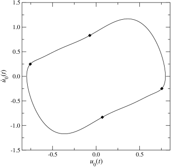
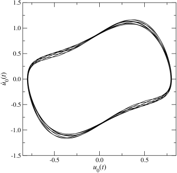
Figure 2: Examples of attractors for $\alpha=2.5$, $\beta=2.0$ and $\mu=0.1$. For $|\omega-4\Omega_{0}|\leq 0.03$ the motion is periodic: in (a), $\omega=4\Omega_{0}+0.02$. The black diamonds mark the four points where $\sin\omega t$ is zero and positive-going. For $\omega=4\Omega_{0}+0.2$ the motion is quasi-periodic (b). Recall that $\Omega_{0}\approx 1.1434$.

We note that for $\Omega_{0}/\omega$ Diophantine the attractor is expected to become quasi-periodic, with the dynamics analytically conjugated to a Diophantine rotation with rotation vector $(\Omega_{0},\omega)$. In principle, this can be proved by KAM techniques [8], or with methods closer to those used in this paper [11, 13, 18, 15, 12].

3 Framework for studying frequency locking

Rescale time so that the driving term has period $2\pi$, hence frequency $1$, by setting $\tau=\omega t$. Then, by denoting with the dot the derivative with respect to rescaled time $\tau$, (2.4) gives

$$\ddot{u}+\frac{1}{\omega}\left(1-\beta+3\beta u^{2}\right)\dot{u}+\frac{1}{\omega^{2}}\left[\left(\alpha-\beta\right)u+\beta\,u^{3}\right]+\mu\bar{\Psi}(u,\dot{u},\tau+\tau_{0})=0,$$ (3.1)

where $\tau_{0}=\omega t_{0}$, and we have defined $\bar{\Psi}(u,\dot{u},\tau)=[\omega^{-1}\,\dot{u}\,(3u^{2}-1)\,\sin\tau$ $+$ $\omega^{-2}(u^{3}-u)\,\sin\tau+\omega^{-1}(u^{3}-u)\,\cos\tau]$. For $\mu=0$ one has $\ddot{u}+\omega^{-1}(1-\beta+3\beta u^{2})\,\dot{u}+\omega^{-2}[(\alpha-\beta)\,u+\beta\,u^{3}]=0$, which can be written as

$$\ddot{u}+\frac{1}{\omega}\,h(u)\,\dot{u}+\frac{1}{\omega^{2}}\,k(u)=0,$$ (3.2)

which is of the form (2.6) up to the rescaling of time. As an effect of the time rescaling, the frequency of the limit cycle for the system (3.2) depends on $\omega$, as it is given by $\overline{\Omega}_{0}=\Omega_{0}/\omega$.

Remark 1

As the solution $u_{0}(\tau)$ is analytic in $\tau$, the property $\dot{u}_{0}(0)=0$ means that we can write $\dot{u}_{0}(\tau)=r_{1}\tau+O(\tau^{2})$, and hence $u_{0}(\tau)=r_{0}+r_{1}\tau^{2}/2+O(\tau^{3})$, with $r_{0}=u_{0}(0)$ and $r_{1}=\ddot{u}_{0}(0)$.

We want to show that if the frequency $\omega$ of the driving term is close to a rational multiple of the unperturbed proper frequency $\Omega_{0}$ of the system, that is $\omega\approx p\Omega_{0}/q$ for some $p,q\in\mathds{N}$ relatively prime, then the frequency $\Omega$ of the solution exactly equals $q\omega/p$, that is $\omega/\Omega=p/q$. Such a phenomenon is known as frequency locking: the system is said to be locked into the resonance $p\!:\!q$.

Let $\rho=p/q\in\mathds{Q}$. For $\mu=0$, for any frequency $\omega$ of the driving term the proper frequency is $\Omega=\Omega_{0}$ — the system is decoupled from the perturbation —, so that if we fix $\omega=\rho\Omega_{0}$ we obtain $\Omega=\Omega_{0}=\omega/\rho$. In terms of the rescaled variables, for which $\omega$ is replaced with $\overline{\omega}=1$, the proper frequency becomes $\overline{\Omega}_{0}=1/\rho$. For $\omega$ close to $\rho\Omega_{0}$ write

$$\frac{1}{\omega}=\frac{1}{\rho\Omega_{0}}+\varepsilon(\mu),$$ (3.3)

with $\varepsilon(\mu)$ such that $\varepsilon(\mu)\to 0$ as $\mu\to 0$.

We look for periodic solutions for the full system (2.4), hence for solutions with period $T=2\pi p/\omega$ (i.e the least common multiple of both $2\pi/\omega$ and $2\pi p/\omega q$). In terms of the rescaled time $\tau$, the solution will have period $2\pi p$, hence frequency $1/p$. For $\mu=0$ the system (3.1) reduces to

$$H_{0}(u,\dot{u},\ddot{u}):=\ddot{u}+f(u)\,\dot{u}+g(u)=0,$$ (3.4)

with

$$f(u)=\frac{1}{\rho\Omega_{0}}\,h(u),\qquad g(u)=\frac{1}{\rho^{2}\Omega_{0}^{2}}\,k(u),$$

which admits the periodic solution $u_{0}(\tau)$ such that $u_{0}(0)>0$, $\dot{u}_{0}(0)=0$ and $u_{0}(\tau+2\pi\rho)=u_{0}(\tau)$. In other words the frequency of the limit cycle is $1/\rho=q/p$ and the period is $2\pi p/q$, i.e. $u_{0}(\tau)=U(\tau/\rho)$, with the function $U$ being $2\pi$-periodic.

For $\mu\neq 0$ we write

$$\varepsilon(\mu)=\varepsilon_{1}\mu+\varepsilon_{2}\mu^{2}+\ldots=\sum_{k=1}^{\infty}\varepsilon_{k}\mu^{k},$$ (3.5)

and, by inserting (3.3) and (3.5) into (3.1), we obtain the equation

$$H(u,\dot{u},\ddot{u},\mu):=H_{0}(u,\dot{u},\ddot{u})+\sum_{k=1}^{\infty}\mu^{k}H_{k}(u,\dot{u},\tau+\tau_{0})=0,$$ (3.6)

where

$$\hbox{}\hskip-19.91684ptH_{1}(u,\dot{u},\tau) = \varepsilon_{1}\left(1-\beta+3\beta u^{2}\right)\dot{u}+\frac{2\varepsilon_{1}}{\rho\Omega_{0}}\left[\left(\alpha-\beta\right)u+\beta\,u^{3}\right]$$ (3.7)

$$+ \frac{1}{\rho\Omega_{0}}\,\dot{u}\left(3u^{2}-1\right)\sin\tau+\frac{1}{\rho^{2}\Omega_{0}^{2}}\left(u^{3}-u\right)\sin\tau+\frac{1}{\rho\Omega_{0}}\left(u^{3}-u\right)\cos\tau,$$

$$\hbox{}\hskip-19.91684ptH_{2}(u,\dot{u},\tau) = \varepsilon_{2}\left(1-\beta+3\beta u^{2}\right)\dot{u}+\left(\frac{2\varepsilon_{2}}{\rho\Omega_{0}}+\varepsilon_{1}^{2}\right)\left[\left(\alpha-\beta\right)u+\beta\,u^{3}\right]$$ (3.8)

$$+ \varepsilon_{1}\dot{u}\left(3u^{2}-1\right)\sin\tau+\frac{2\varepsilon_{1}}{\rho\Omega_{0}}\left(u^{3}-u\right)\sin\tau+\varepsilon_{1}\left(u^{3}-u\right)\cos\tau,$$

and so on. The shifting of time by $\tau_{0}=\omega t_{0}$ in the driving term is due to the choice of the origin of time made according to Section 2.

In the following sections we shall prove that for $\mu$ small enough it is possible to choose $\varepsilon(\mu)$ as a function of $t_{0}$, in such a way that there exists a periodic solution of (3.6) with period $2\pi p$, i.e. with frequency $1/p$. When projected onto the $(u,\dot{u})$ plane, such a solution is close enough to the unperturbed limit cycle (cf. for instance Figure 2): the difference between them is of order $\mu$.

4 The linearised equation

Write the unperturbed system (3.4) as

$$\dot{u}=v,\qquad\dot{v}=G(u,v),$$ (4.1)

with $G(u,v)=-(\rho\Omega_{0})^{-1}(1-\beta+3\beta u^{2})\,v-(\rho^{2}\Omega_{0})^{-2}[(\alpha-\beta)\,u+\beta\,u^{3}]$. Let $(u_{0}(\tau),v_{0}(\tau))$ be the $2\pi\rho$-periodic solution of (4.1), which is uniquely determined by the conditions

$$\dot{u}_{0}(0)=0,\qquad u_{0}(0)>0.$$ (4.2)

The periodicity properties of $u_{0}(\tau)$ allow us to write

$$u_{0}(\tau)=\sum_{\begin{subarray}{c}{\nu\in\mathds{Z}}\\ \nu\;{\rm odd}\end{subarray}}{\rm e}^{i\nu\tau/\rho}u_{0,\nu},\qquad\rho=\frac{p}{q},$$ (4.3)

as follows from Lemma 1. Denote by

$$W(\tau)=\left(\begin{matrix}w_{11}(\tau)&w_{12}(\tau)\\ w_{21}(\tau)&w_{22}(\tau)\end{matrix}\right)$$ (4.4)

the Wronskian matrix of the system (4.1), that is the solution of the matrix equation

$$\begin{cases}\dot{W}(\tau)=M(\tau)\,W(\tau),&\\ W(0)=\mathds{1},\end{cases}\qquad M(\tau)=\left(\begin{matrix}0&1\\ G_{u}(u_{0}(\tau),v_{0}(\tau))&G_{v}(u_{0}(\tau),v_{0}(\tau))\end{matrix}\right),$$ (4.5)

where $G_{u}$ and $G_{v}$ denote derivatives with respect to $u$ and $v$ of $G$, and $w_{21}(\tau)=\dot{w}_{11}(\tau)$, $w_{22}(\tau)=\dot{w}_{12}(\tau)$.

Lemma 3

In (4.4) one can set

$$w_{12}(\tau):=c_{2}\dot{u}_{0}(\tau),\qquad w_{11}(\tau):=c_{1}\dot{u}_{0}(\tau)\int_{\bar{\tau}}^{\tau}{\rm d}\tau^{\prime}\frac{{\rm e}^{-F(\tau^{\prime})}}{\dot{u}_{0}^{2}(\tau^{\prime})},$$ (4.6)

where $F(\tau)$ is defined as

$$F(\tau):=\int_{0}^{\tau}{\rm d}\tau^{\prime}\,f(u_{0}(\tau^{\prime})),\qquad f(u):=\frac{1}{\rho\Omega_{0}}\left(1-\beta+3\beta u^{2}\right)=\frac{1}{\rho\Omega_{0}}\,h(u),$$ (4.7)

the constant $\bar{\tau}\in(0,\pi\rho)$ is chosen so that $\dot{w}_{11}(0)=0$, and the constants $c_{1}$ and $c_{2}$ are such that $w_{11}(0)=w_{22}(0)=1$.

Proof. It can immediately be checked that $(w_{12}(\tau),w_{22}(\tau))$, with $w_{12}(\tau)$ defined as in (4.6) and $w_{22}(\tau)=\dot{w}_{12}(\tau)$, solves the linearised equation to (4.1). Then a second independent solution is of the form $(w_{11}(\tau),w_{21}(\tau))$, with $w_{11}(\tau)$ given by (4.6) and $w_{21}(\tau)=\dot{w}_{11}(\tau)$; cf. [23], p. 122. In Appendix A we show that it is possible to choose $\bar{\tau}\in(0,\pi\rho)$ in such a way that $\dot{w}_{11}(0)=0$. The constants $c_{1}$ and $c_{2}$ are chosen so that $W(0)=\mathds{1}$.  

Remark 2

With the notations of Remark 1 one has $c_{2}=1/r_{1}$ and $c_{1}=-r_{1}$, so that $c_{1}c_{2}+1=0$.

Note that $\dot{u}_{0}(0)=0$, so that in (4.6) the function $w_{11}(\tau)$ at $\tau=0$ is defined as the limit

$$\lim_{\tau\to 0}c_{1}\dot{u}_{0}(\tau)\int_{\bar{\tau}}^{\tau}{\rm d}\tau^{\prime}\frac{{\rm e}^{-F(\tau^{\prime})}}{\dot{u}_{0}^{2}(\tau^{\prime})},$$ (4.8)

which is well defined; cf. Appendix A. The same argument applies for $\tau=\pi\rho$, where $\dot{u}_{0}(\pi\rho)=\dot{u}_{0}(0)=0$ — by (2.8), with the half-period $T_{0}/2$ becoming $\pi\rho$ in terms of the rescaled variable.

For any periodic function $G$ we denote its average by $\langle G\rangle$ and set $\tilde{G}=G-\langle G\rangle$. Then $f_{0}:=\langle f\circ u_{0}\rangle>0$ (cf. Lemma 2), so that we can write

$${\rm e}^{-F(\tau)}={\rm e}^{-f_{0}\tau-\tilde{F}(\tau)},\qquad\tilde{F}(\tau)=\int_{0}^{\tau}{\rm d}\tau^{\prime}\left(f(u_{0}(\tau^{\prime}))-f_{0}\right),$$ (4.9)

where $\tilde{F}(\tau)$, and hence ${\rm e}^{-\tilde{F}(\tau)}$, are well defined $2\pi\rho\,$-periodic functions.

Lemma 4

Given any periodic function $P(\tau)$ and any real constant $C\neq 0$ there exists a periodic function $Q(\tau)$, with the same period as $P(\tau)$, and a constant $D$ such that

$$\int_{0}^{\tau}{\rm d}\tau^{\prime}\,{\rm e}^{C\tau^{\prime}}P(\tau^{\prime})=D+{\rm e}^{C\tau}Q(\tau).$$

One has $D=-Q(0)$.

Proof. Let $P(\tau)$ be a periodic function of period $T$. Write

$$P(\tau)=\sum_{\nu\in\mathds{Z}}{\rm e}^{i\omega\nu\tau}P_{\nu},$$ (4.10)

where $\omega=2\pi/T$. Then one has

$$\int_{0}^{\tau}{\rm d}\tau^{\prime}\,{\rm e}^{C\tau^{\prime}}P(\tau^{\prime})=\sum_{\nu\in\mathds{Z}}P_{\nu}\int_{0}^{\tau}{\rm d}\tau^{\prime}\,{\rm e}^{i\omega\nu\tau^{\prime}+C\tau^{\prime}}=\sum_{\nu\in\mathds{Z}}P_{\nu}\frac{{\rm e}^{i\omega\nu\tau+C\tau}-1}{C+i\omega\nu},$$

so that, by setting

$$Q(\tau):=\sum_{\nu\in\mathds{Z}}\frac{P_{\nu}}{C+i\omega\nu}{\rm e}^{i\omega\nu\tau},\qquad D:=-\sum_{\nu\in\mathds{Z}}\frac{P_{\nu}}{C+i\omega\nu},$$ (4.11)

the assertion follows.  

Lemma 5

There exist two $2\pi\rho$-periodic functions $a(\tau)$ and $b(\tau)$ such that

$$w_{11}(\tau)=a(\tau)+{\rm e}^{-f_{0}\tau}\,b(\tau),\qquad w_{12}(\tau)=c\,a(\tau),$$ (4.12)

for a suitable constant $c$.

Proof. We cannot directly apply Lemma 4 because the function ${\rm e}^{-F(\tau)}/\dot{u}_{0}^{2}(\tau)$ appearing in (4.6) is singular. However we can proceed as follows. We write

$$\frac{1}{\dot{u}_{0}^{2}(\tau)}=\lim_{\eta\to 0}\frac{1}{\dot{u}_{0}^{2}(\tau)+\eta},$$

so that the new integrand is smooth and it is given by ${\rm e}^{-f_{0}\tau}$ times a $2\pi\rho$-periodic function. Hence, as long as $0<\tau<\pi\rho$, the integrand is bounded uniformly in $\eta$, and we can apply Lebesgue’s dominated convergence theorem, to write

$$w_{11}(\tau)=c_{1}\dot{u}_{0}(\tau)\lim_{\eta\to 0}\int_{\bar{\tau}}^{\tau}{\rm d}\tau^{\prime}\,\frac{{\rm e}^{ct^{\prime}}}{\dot{u}_{0}^{2}(\tau^{\prime})+\eta}.$$

Then Lemma 4 gives

$$w_{11}(\tau)=c_{1}\dot{u}_{0}(\tau)\lim_{\eta\to 0}\left({\rm e}^{c\tau}P(\tau,\eta)-{\rm e}^{c\bar{\tau}}P(\bar{\tau},\eta)\right)=c_{1}\lim_{\eta\to 0}\left(\dot{u}_{0}(\tau){\rm e}^{c\tau}P(\tau,\eta)\right)-\dot{u}_{0}(\tau){\rm e}^{c\bar{\tau}}P(\bar{\tau}),$$

where the function $P(\tau,\eta)$ is $2\pi\rho\,$-periodic in $\tau$ and $P(\bar{\tau})=\lim_{\eta\to 0}P(\bar{\tau},\eta)$ is well defined. Note that $-\dot{u}_{0}(\tau){\rm e}^{c\bar{\tau}}P(\bar{\tau})$ gives the function $a(\tau)$ in (4.12). On the other hand, the function $w_{11}(\tau)$ is also well defined, so that we can conclude that $\lim_{\eta\to 0}\left(\dot{u}_{0}(\tau){\rm e}^{c\tau}P(\tau,\eta)\right)$ is well defined and smooth. As the function $\dot{u}_{0}(\tau)\,P(\tau,\eta)$ is periodic for any $\eta$, the limit will also be periodic, and this defines the function $b(\tau)$ of (4.12).

Comparing the expressions for $w_{11}(\tau)$ and $w_{12}(\tau)$ in (4.6), proportionality between the function $w_{12}(\tau)$ and the periodic component of $w_{11}(\tau)$ also follows.  

Lemma 6

The Fourier expansions of the functions $a(\tau)$ and $b(\tau)$ in (4.12) contain only the odd harmonics.

Proof. Write $u_{0}(\tau)$ according to (4.3). Then $w_{12}(\tau)=c\,a(\tau)=c\,\dot{u}_{0}(\tau)$, so that the assertion follows trivially for $a(\tau)$. Moreover the function ${\rm e}^{-F(\tau)}/\dot{u}_{0}^{2}(\tau)$ involves even powers of functions containing only odd harmonics, so that it contains only even harmonics, and so does its integral as appearing in the definition (4.6) of $w_{11}(\tau)$. Hence, by Lemma 4 and Lemma 5, also $b(\tau)$ in (4.12) contains only the odd harmonics.  

A straightforward calculation gives $\det W(\tau)=-c_{1}c_{2}{\rm e}^{-F(\tau)}={\rm e}^{-F(\tau)}$, since $c_{1}c_{2}=-1$, so that

$$W^{-1}(\tau)={\rm e}^{F(\tau)}\left(\begin{matrix}w_{22}(\tau)&-w_{12}(\tau)\\ -w_{21}(\tau)&w_{11}(\tau)\end{matrix}\right).$$ (4.13)

We want to develop perturbation theory for a $2\pi p$-periodic solution which continues the solution running on the unperturbed limit cycle when the perturbation is switched on. Therefore we write

$$u(\tau)=u_{0}(\tau)+\sum_{k=1}^{\infty}\mu^{k}u_{k}(\tau),\qquad u_{k}(\tau)=\sum_{\nu\in\mathds{Z}}{\rm e}^{i\nu\tau/p}u_{k,\nu},$$ (4.14)

where $u_{0}(\tau)$ is the solution satisfying the conditions (4.2). Inserting (4.14) into (3.6) and expanding everything in powers of $\mu$, we obtain a sequence of recursive equations. In Sections 5 and 6 we shall consider in detail the first order. Higher order analysis and the issue of convergence will be discussed in Section 7.

5 First order computations

Let us also expand the initial conditions in $\mu$:

$$u(0):=\bar{u}=u_{0}(0)+\sum_{k=1}^{\infty}\mu^{k}\bar{u}_{k},\qquad\dot{u}(0):=\bar{v}=\sum_{k=1}^{\infty}\mu^{k}\bar{v}_{k},$$ (5.1)

and set $\Psi_{1}(\tau)=H_{1}(u_{0}(\tau),v_{0}(\tau),\tau+\tau_{0})$ — cf. (3.7). We look for a solution $(u(\tau),v(\tau))$ which is analytic in $\mu$, i.e. $u(\tau)=u_{0}(\tau)+\mu u_{1}(\tau)+\mu^{2}u_{2}(\tau)+\ldots$ and $v(\tau)=\dot{u}(\tau)$ — cf. [4, 6, 17] for similar situations. Here we are interested in the dynamics on the attractor, hence in periodic solutions, but in principle we could also study the dynamics near the attractor, by looking for solutions of the form $u(\tau)=U({\rm e}^{-f_{1}\tau},{\rm e}^{-f_{2}\tau},\tau)$, as in [11, 13, 5], with $f_{1}=f_{0}+O(\mu)$ and $f_{2}=O(\mu)$, and $U(\cdot,\cdot,\psi)$ $2\pi/p$-periodic in $\psi$. To first order one has

$$\left(\begin{matrix}u_{1}(\tau)\\ v_{1}(\tau)\end{matrix}\right)=W(\tau)\left[\left(\begin{matrix}\bar{u}_{1}\\ \bar{v}_{1}\end{matrix}\right)+\int_{0}^{\tau}{\rm d}\tau^{\prime}\,W^{-1}(\tau^{\prime})\left(\begin{matrix}0\\ \Psi_{1}(\tau^{\prime})\end{matrix}\right)\right],$$ (5.2)

and we can confine ourselves to the first component $u_{1}(\tau)$, since $v_{1}(\tau)=\dot{u}_{1}(\tau)$,

$$u_{1}(\tau)=w_{11}(\tau)\,\bar{u}_{1}+w_{12}(\tau)\,\bar{v}_{1}+\int_{0}^{\tau}{\rm d}\tau^{\prime}\,{\rm e}^{F(\tau^{\prime})}\left[w_{12}(\tau)w_{11}(\tau^{\prime})-w_{11}(\tau)w_{12}(\tau^{\prime})\right]\Psi_{1}(\tau).$$

which can be more conveniently written as

$$u_{1}(\tau)=w_{11}(\tau)\left(\bar{u}_{1}\!\!-\int_{0}^{\tau}\!\!\!\!{\rm d}\tau^{\prime}\,{\rm e}^{F(\tau^{\prime})}w_{12}(\tau^{\prime})\Psi_{1}(\tau^{\prime})\right)+w_{12}(\tau)\left(\bar{v}_{1}+\!\!\int_{0}^{\tau}\!\!\!\!{\rm d}\tau^{\prime}\,{\rm e}^{F(\tau^{\prime})}w_{11}(\tau^{\prime})\Psi_{1}(\tau^{\prime})\right).$$

The function ${\rm e}^{F(\tau)}w_{11}(\tau)\Psi_{1}(\tau)$ is periodic, while ${\rm e}^{F(\tau)}w_{12}(\tau)\Psi_{1}(\tau)$ is given by ${\rm e}^{f_{0}\tau}$ times a periodic function. Therefore we can write $w_{11}(\tau)$ and $w_{12}(\tau)$ according to (4.6), and set — cf. Lemma 4 —

$$\int_{0}^{\tau}{\rm d}\tau^{\prime}\,{\rm e}^{F(\tau^{\prime})}a(\tau^{\prime})\Psi_{1}(\tau^{\prime}) = {\rm e}^{f_{0}\tau}{\mathcal{Q}}_{1}(\tau)-{\mathcal{Q}}_{1}(0),$$ (5.3)

$$\int_{0}^{\tau}{\rm d}\tau^{\prime}\,{\rm e}^{F(\tau^{\prime})}{\rm e}^{-f_{0}\tau^{\prime}}b(\tau^{\prime})\Psi_{1}(\tau^{\prime}) = \tau{\mathcal{Q}}_{0}+{\mathcal{Q}}_{2}(\tau)-{\mathcal{Q}}_{2}(0),$$ (5.4)

for some periodic functions ${\mathcal{Q}}_{1}(\tau)$ and ${\mathcal{Q}}_{2}(\tau)$, and with

$${\mathcal{Q}}_{0}=\langle{\rm e}^{\tilde{F}}b\,\Psi_{1}\rangle.$$ (5.5)

Assume that we can choose the parameters in such a way that ${\mathcal{Q}}_{0}=0$. Then we obtain

$$u_{1}(\tau)\!\!\! = \!\!\!a(\tau)\left(\bar{u}_{1}+c{\mathcal{Q}}_{1}(0)-{\rm e}^{f_{0}\tau}c\,{\mathcal{Q}}_{1}(\tau)+c\,\bar{v}_{1}+{\rm e}^{f_{0}\tau}c\,{\mathcal{Q}}_{1}(\tau)-c\,{\mathcal{Q}}_{1}(0)\right.$$ (5.6)

$$\!\!\!+ \!\!\!{\mathcal{Q}}_{2}(\tau)-{\mathcal{Q}}_{2}(0)\left)\;+\;\;{\rm e}^{-f_{0}\tau}b(\tau)\left(\bar{u}_{1}+c\,{\mathcal{Q}}_{1}(0)-{\rm e}^{f_{0}\tau}c\,{\mathcal{Q}}_{1}(\tau)\right)\right.,$$

and if we want that (5.6) describe a periodic function, the constant $\bar{v}_{1}$ can assume any value, but we need

$$\bar{u}_{1}=-c\,{\mathcal{Q}}_{1}(0).$$ (5.7)

so that (5.6) becomes

$$u_{1}(\tau)=a(\tau)\left(c\,\bar{v}_{1}-c\,{\mathcal{Q}}_{1}(0)+{\mathcal{Q}}_{2}(\tau)-{\mathcal{Q}}_{2}(0)\right)+c\,b(\tau){\mathcal{Q}}_{1}(\tau),$$ (5.8)

where we have used that the function ${\rm e}^{f_{0}\tau}c\,{\mathcal{Q}}_{1}(\tau)$ appears twice but with opposite sign in (5.6).

Remark 3

The constant $\bar{v}_{1}$ is left undetermined, and we can fix it arbitrarily, say $\bar{v}_{1}=0$, as we still have at our disposal the free parameter $\tau_{0}$; cf. [17], Section 2, for an analogous discussion.

Therefore we can conclude that if ${\mathcal{Q}}_{0}=0$ then we can choose $\bar{u}_{1}$ according to (5.7) in such a way that up to first order there exists a periodic solution $u_{0}(\tau)+\mu u_{1}(\tau)+O(\mu^{2})$. In the next Section we study in detail the condition ${\mathcal{Q}}_{0}=0$.

6 Compatibility to first order

Consider the equation ${\mathcal{Q}}_{0}=0$, which can be written as

$$\varepsilon_{1}A+B_{1}(\tau_{0})+B_{2}(\tau_{0})+B_{3}(\tau_{0})=0,$$ (6.1)

where we have defined

$$A\!\! := \!\!\left\langle{\rm e}^{\tilde{F}}b\left[\left(1-\beta+3\beta u_{0}^{2}\right)\dot{u}_{0}+\frac{2}{\rho\Omega_{0}}\left(\alpha u_{0}-\beta u_{0}+\beta\,u_{0}^{3}\right)\right]\right\rangle$$ (6.2)

$$= \!\!\frac{1}{2\pi p}\int_{0}^{2\pi p}{\rm d}\tau\,{\rm e}^{\tilde{F}(\tau)}b(\tau)\left[\dot{u}_{0}(\tau)\,h(u_{0}(\tau))+\frac{2}{\rho\Omega_{0}}k(u_{0}(\tau))\right]$$

$$= \!\!\frac{1}{2\pi\rho}\int_{0}^{2\pi\rho}{\rm d}\tau\,{\rm e}^{\tilde{F}(\tau)}b(\tau)\left[\dot{u}_{0}(\tau)\,h(u_{0}(\tau))+\frac{2}{\rho\Omega_{0}}k(u_{0}(\tau))\right],$$

and

$$B_{1}(\tau_{0}) := \frac{1}{2\pi p}\int_{0}^{2\pi p}{\rm d}\tau\,{\rm e}^{\tilde{F}(\tau)}b(\tau)\left[\frac{1}{\rho\Omega_{0}}\dot{u}_{0}(\tau)\left(3u_{0}^{2}(\tau)-1\right)\right]\sin(\tau+\tau_{0}),$$

$$B_{2}(\tau_{0}) := \frac{1}{2\pi p}\int_{0}^{2\pi p}{\rm d}\tau\,{\rm e}^{\tilde{F}(\tau)}b(\tau)\left[\frac{1}{\rho^{2}\Omega_{0}^{2}}u_{0}(\tau)\left(u_{0}^{2}(\tau)-1\right)\right]\sin(\tau+\tau_{0}),$$

$$B_{3}(\tau_{0}) := \frac{1}{2\pi p}\int_{0}^{2\pi p}{\rm d}\tau\,{\rm e}^{\tilde{F}(\tau)}b(\tau)\left[\frac{1}{\rho\Omega_{0}}u_{0}(\tau)\left(u_{0}^{2}(\tau)-1\right)\right]\cos(\tau+\tau_{0}).$$ (6.3)

Remark 4

Note that we can write (6.2) as $A=\frac{1}{2\pi\rho}\int_{0}^{2\pi}{\rm d}s\,Q(s)\left[\frac{{\rm d}U(s)}{{\rm d}s}\,h(U(s))+\frac{2}{\Omega_{0}}k(U(s))\right]$, where $U(s)$ and $Q(s)$ are $2\pi$-periodic functions, with $U(s)=u_{0}(\rho s)$ and $Q(s)={\rm e}^{\tilde{F}(\rho s)}\,b(\rho s)$. The function $U(s)$ is the $2\pi$-periodic solution of the differential equation ${\rm d}^{2}U/{\rm d}s^{2}+\Omega_{0}^{-1}h(U)\,{\rm d}U/{\rm d}s+\Omega_{0}^{-2}k(U)=0$, and $\tilde{F}(\rho s)=-\frac{f_{0}\,s}{\Omega_{0}}+\frac{1}{\Omega_{0}}\int_{0}^{s}{\rm d}s^{\prime}\,h(U(s^{\prime}))$, so that the constant $A$ is of the form $A=\bar{A}/\rho$, with $\bar{A}$ independent of $\rho$. Hence if $A\neq 0$ for some $\rho\in\mathds{Q}$ then it is non-zero for all rational $\rho\neq 0$.

By expanding $\sin(\tau+\tau_{0})=\sin\tau\cos\tau_{0}+\cos\tau\sin\tau_{0}$ and $\cos(\tau+\tau_{0})=\cos\tau\cos\tau_{0}-\sin\tau\sin\tau_{0}$, we can rewrite (6.3) as $B_{i}(\tau_{0})=B_{i1}\cos\tau_{0}+B_{i2}\sin\tau_{0}$ for $i=1,2,3$, where we have introduced the constants

$$B_{11}\!\!\! := \!\!\!\frac{1}{2\pi p}\int_{0}^{2\pi p}{\rm d}\tau\,{\rm e}^{\tilde{F}(\tau)}b(\tau)\left[\frac{1}{\rho\Omega_{0}}\dot{u}_{0}(\tau)\left(3u_{0}^{2}(\tau)-1\right)\right]\sin\tau,$$

$$B_{12}\!\!\! := \!\!\!\frac{1}{2\pi p}\int_{0}^{2\pi p}{\rm d}\tau\,{\rm e}^{\tilde{F}(\tau)}b(\tau)\left[\frac{1}{\rho\Omega_{0}}\dot{u}_{0}(\tau)\left(3u_{0}^{2}(\tau)-1\right)\right]\cos\tau,$$

$$B_{21}\!\!\! := \!\!\!\frac{1}{2\pi p}\int_{0}^{2\pi p}{\rm d}\tau\,{\rm e}^{\tilde{F}(\tau)}b(\tau)\left[\frac{1}{\rho^{2}\Omega_{0}^{2}}u_{0}(\tau)\left(u_{0}^{2}(\tau)-1\right)\right]\sin\tau=-\rho\Omega_{0}B_{32},$$

$$B_{22}\!\!\! := \!\!\!\frac{1}{2\pi p}\int_{0}^{2\pi p}{\rm d}\tau\,{\rm e}^{\tilde{F}(\tau)}b(\tau)\left[\frac{1}{\rho^{2}\Omega_{0}^{2}}u_{0}(\tau)\left(u_{0}^{2}(\tau)-1\right)\right]\cos\tau=\rho\Omega_{0}B_{31}.$$ (6.4)

By setting $D_{1}=-\left(B_{11}+B_{21}+B_{31}\right)$ and $D_{2}=-\left(B_{12}+B_{22}+B_{32}\right)$, (6.1) then becomes

$$\varepsilon_{1}A={\mathfrak{D}}_{1}(\tau_{0}):=D_{1}\cos\tau_{0}+D_{2}\sin\tau_{0}.$$ (6.5)

All constants $B_{ij}$ in (6.4) are given by the average of a suitable function which can be written as the product of a $2\pi/\rho\,$-periodic function times a cosine or sine function. Consider explicitly the constant $B_{11}$; the other constants can be discussed in the same way. We write

$$B_{11}=\frac{1}{2\pi p}\int_{0}^{2\pi p}{\rm d}\tau\,K(\tau)\,\sin\tau,\qquad\text{with}\qquad K(\tau)=\sum_{\begin{subarray}{c}\nu\in\mathds{Z}\\ \nu\;{\rm even}\end{subarray}}{\rm e}^{i\nu\tau/\rho}K_{\nu}=\sum_{\nu\in\mathds{Z}}{\rm e}^{i2\nu\tau/\rho}K_{2\nu},$$

as follows from Lemmas 3 and 6. If we write $\sin\tau=\sum_{\sigma=\pm 1}(\sigma/2i){\rm e}^{i\sigma\tau}$, then

$$B_{11}=\sum_{\begin{subarray}{c}\nu\in\mathds{Z},\,\sigma=\pm 1\\ 2\nu+\sigma\rho=0\end{subarray}}\frac{\sigma K_{2\nu}}{2i}.$$ (6.6)

The same argument applies to the other constants, so that we can conclude that the constants $B_{ij}$ can be different from zero only if $\rho$ is an even integer. If we set $\rho=p/q$ this means $q=1$ and $p=2n$, $n\in\mathds{N}$. Hence for all rational $\rho\notin 2\mathds{N}$ the first order compatibility equation (6.5) gives $\varepsilon_{1}A=0$, so that either $A=0$ and $\varepsilon_{1}$ is arbitrary or $A\neq 0$ and $\varepsilon_{1}=0$. An explicit calculation (cf. Appendix B) shows that $A\neq 0$. Therefore for all resonances $p\!:\!q$, with $p/q\notin 2\mathds{N}$, frequency locking, if possible at all, can occur only for a range of frequencies of width at most $\mu^{2}$.

The argument above does not imply that $D_{1},D_{2}\neq 0$ for $p/q\in 2\mathds{N}$ — in principle there could be cancellations in the sum (6.6). For any given resonance $p\!:\!q$, the non-vanishing of the constants $D_{1}$ and $D_{2}$ can be checked numerically; for instance, when $\alpha=5$ and $\beta=4$, for $p/q=2$ one finds $D_{1}=0.00735$ and $D_{2}=-0.04507$ [7]. Therefore for $\rho=2n$, $n\in\mathds{N}$, frequency locking occurs for a range of frequencies of width of order $\mu$ around the value $2n$.

7 Higher order computations and convergence

To extend the analysis of the previous sections to any perturbation order, we write the solution we are looking for as

$$u(\tau)=\sum_{k=0}^{\infty}\mu^{k}u_{k}(\tau),\qquad v(\tau)=\sum_{k=0}^{\infty}\mu^{k}v_{k}(\tau)=\dot{u}(\tau),$$ (7.1)

with $(u(0),v(0))$ written according to (5.1). Thus we find for all $k\in\mathds{N}$

$$\left(\begin{matrix}u_{k}(\tau)\\ v_{k}(\tau)\end{matrix}\right)=W(\tau)\left[\left(\begin{matrix}\bar{u}_{k}\\ \bar{v}_{k}\end{matrix}\right)+\int_{0}^{\tau}{\rm d}\tau^{\prime}\,W^{-1}(\tau^{\prime})\left(\begin{matrix}0\\ \Psi_{k}(\tau^{\prime})\end{matrix}\right)\right],$$ (7.2)

where

$$\Psi_{k}(\tau):=\left[\sum_{k^{\prime}=1}^{k}\mu^{k^{\prime}}H_{k^{\prime}}(u(\tau),\dot{u}(\tau),\tau+\tau_{0})\right]_{k},$$ (7.3)

with $H_{k}$ defined in (3.6). The notation $[\cdot]_{k}$ for $\Psi_{k}(\tau)$ in (7.3) means the following. In each term $H_{k^{\prime}}$, we expand $u(\tau)$ and $\dot{u}(\tau)$ according to (7.1), and, by taking the Taylor series of the function $H_{k^{\prime}}$, we keep all contributions proportional to $\mu^{k}$: we write the sum of these contributions as $\mu^{k}\Psi_{k}(\tau)$. For instance one has $\Psi_{2}(\tau)=H_{2}(u_{0}(\tau),v_{0}(\tau),\tau+\tau_{0})+\frac{\partial}{\partial u_{0}}H_{1}(u_{0}(\tau),v_{0}(\tau),\tau+\tau_{0})\,u_{1}(\tau)+\frac{\partial}{\partial v_{0}}H_{1}(u_{0}(\tau),v_{0}(\tau),\tau+\tau_{0})\,\dot{u}_{1}(\tau)$, with $u_{1}(\tau)$ given by (5.8).

As in Section 5, we study only the equation for the first component, which is

$$u_{k}(\tau)=w_{11}(\tau)\,\bar{u}_{k}+w_{12}(\tau)\,\bar{v}_{k}+\int_{0}^{\tau}{\rm d}\tau^{\prime}\,{\rm e}^{F(\tau^{\prime})}\left[w_{12}(\tau)w_{11}(\tau^{\prime})-w_{11}(\tau)w_{12}(\tau^{\prime})\right]\Psi_{k}(\tau^{\prime}).$$ (7.4)

The equation (7.4) for $k=1$ has been studied in Section 5. Here we want to show that the equation (7.4) is well defined to any perturbation order $k$, and that it is possible to choose the constant $\varepsilon_{k}$ in (3.5) so that it admits a periodic solution $u_{k}(\tau)$.

The discussion proceeds as in Section 5, once we note that each function $H_{k}(u,\dot{u},\tau+\tau_{0})$ in (3.6) contains a term $\varepsilon_{k}\left(1-\beta+3\beta u^{2}\right)\dot{u}+2\varepsilon_{k}(\rho\Omega_{0})^{-1}\left[\left(\alpha-\beta\right)u+\beta\,u^{3}\right]$, whereas all the other terms depend on the constants $\varepsilon_{k^{\prime}}$, with $k^{\prime}$ strictly less than $k$. Therefore for $k\in\mathds{N}$ one has

$$\Psi_{k}(\tau)=\varepsilon_{k}\left(1-\beta+3\beta u_{0}^{2}\right)\dot{u}_{0}(\tau)+\frac{2\varepsilon_{k}}{\rho\Omega_{0}}\left[\left(\alpha-\beta\right)u_{0}(\tau)+\beta\,u_{0}^{3}(\tau)\right]+\Xi_{k}(\tau;\tau_{0}),$$ (7.5)

with the function $\Xi_{k}(\tau;\tau_{0})$ depending only on the constants $\varepsilon_{1},\ldots,\varepsilon_{k-1}$, besides the parameter $\tau_{0}$ and time $\tau$. Therefore to any perturbation order $k$, in order to have a periodic solution, we need

$${\mathcal{Q}}_{k,0}:=\langle{\rm e}^{\tilde{F}}b\,\Psi_{k}\rangle=0,$$ (7.6)

and this can be obtained by requiring

$$\varepsilon_{k}A={\mathfrak{D}}_{k}(\tau_{0}),\qquad{\mathfrak{D}}_{k}(\tau_{0}):=-\langle{\rm e}^{\tilde{F}}b\,\Xi_{k}(\cdot;\tau_{0})\rangle,$$ (7.7)

with $A$ defined as in (6.2). Since $A\neq 0$ (as proved in Appendix B) then we can use (7.7) to fix $\varepsilon_{k}$ as a function of $\tau_{0}$. Defining the periodic functions ${\mathcal{Q}}_{k,1}(\tau)$ and ${\mathcal{Q}}_{k,2}(\tau)$ such that

$$\int_{0}^{\tau}{\rm d}\tau^{\prime}\,{\rm e}^{F(\tau^{\prime})}a(\tau^{\prime})\Psi_{k}(\tau^{\prime}) = {\rm e}^{f_{0}\tau}{\mathcal{Q}}_{k,1}(\tau)-{\mathcal{Q}}_{k,1}(0),$$ (7.8)

$$\int_{0}^{\tau}{\rm d}\tau^{\prime}\,{\rm e}^{F(\tau^{\prime})}{\rm e}^{-f_{0}\tau^{\prime}}b(\tau^{\prime})\Psi_{k}(\tau^{\prime}) = \tau{\mathcal{Q}}_{k,0}+{\mathcal{Q}}_{k,2}(\tau)-{\mathcal{Q}}_{k,2}(0),$$ (7.9)

choosing the constants $\bar{u}_{k}$ so that $\bar{u}_{k}+c{\mathcal{Q}}_{k,1}(0)=0$, and using (7.6), then (7.4) gives

$$u_{k}(\tau)=a(\tau)\left(c\,\bar{v}_{k}-c\,{\mathcal{Q}}_{k,1}(0)+{\mathcal{Q}}_{k,2}(\tau)-{\mathcal{Q}}_{k,2}(0)\right)+c\,b(\tau){\mathcal{Q}}_{k,1}(\tau),$$ (7.10)

with the constants $\bar{v}_{k}$ which will be fixed in the most convenient way (cf. Remark 3). For instance we can set $\bar{v}_{k}=0$ for all $k\in\mathds{N}$.

We can make the perturbative analysis of the previous sections rigorous to all orders, by following the strategy introduced in [17, 6], and hence study the convergence of the perturbation series. Alternatively, one could try to apply arguments based on the implicit function theorems. Typically, the latter would allow a simplification of the proof of existence of the periodic solutions, but would be less suitable for explicitly constructing the solutions themselves within any given accuracy; see the comments in [17]; therefore we follow the first method. Note that we are not confining ourselves to approximate analytical solutions, which could be unreliable because of the uncontrolled truncation of the series expansion. On the contrary we want also to settle the issue of convergence. In some sense this approach is complementary to that of [19], where qualitative geometric methods are preferred to quantitative analytical ones.

The study of the convergence of the series is standard, and it has been discussed extensively and in full detail in [17] for a similar situation. Thus, we only sketch how the argument proceeds.

By expanding the functions $u(\tau)$ and $\dot{u}(\tau)$ in $H_{k^{\prime}}(u(\tau),\dot{u}(\tau),\tau+\tau_{0})$ in (7.3) according to (7.1), one sees that $\Psi_{k}(\tau)$ can be expressed in terms of the functions $u_{k^{\prime}}(\tau)$ with $k^{\prime}<k$. On the other hand, by (7.10), the functions $u_{k}(\tau)$ are expressed in terms of the functions ${\mathcal{Q}}_{k,1}(\tau)$ and ${\mathcal{Q}}_{k,2}(\tau)$, which in turn are integrals of functions involving $\Psi_{k}(\tau)$, and hence depend on $u_{k^{\prime}}(\tau)$ for $k^{\prime}<k$.

This means that we have recursive equations for the functions $u_{k}(\tau)$. By passing to the Fourier space, that is by expanding $u_{k}(\tau)=\sum_{\nu\in\mathds{Z}}{\rm e}^{i\nu\tau/p}u_{k,\nu}$, we obtain recursive equations for the Fourier coefficients $u_{k,\nu}$. We do not write them explicitly because the ensuing expressions are rather cumbersome, but one can easily work out the analytical expressions for the recursions by following the scheme that we have outlined. Eventually, we can represent $u_{k,\nu}$ for $k\geq 1$ and $\nu\in\mathds{Z}$, in terms of tree graphs, which can be studied with the techniques of [17].

We do not repeat the analysis here, but we instead just give the final result. To any order $k\geq 1$ one obtain the following bounds for the Fourier coefficients: $|u_{k,\nu}|\leq C_{1}C_{2}^{k-1}$ and $\sum_{\nu\in\mathds{Z}}|u_{k,\nu}|\leq C_{3}C_{2}^{k-1}$, for suitable positive constants $C_{1},C_{2},C_{3}$, depending on $\rho$. This implies the convergence of the perturbation series (7.1) for $\mu$ small enough, say for $|\mu|<C_{2}^{-1}$.

8 Arnold tongues and devil’s staircase

We use the perturbative analysis, developed to all orders in the previous section, to study for which values of the driving frequency $\omega$ one has locking. We shall see that the analysis accounts for the devil’s staircase structure found in [29], for small values of the driving amplitude $\mu$.

Lemma 7

The functions $H_{k}(u,\dot{u},\tau+\tau_{0})$ in (3.6) are polynomials of odd order in $(u,\dot{u})$ for all $k\in\mathds{N}$.

Proof. The function $H(u,\dot{u},\ddot{u},\mu)$ given by (3.1) is a polynomial of odd order in $(u,\dot{u},\ddot{u})$. By writing $H(u,\dot{u},\ddot{u},\mu)$ as in (3.6), the only term containing $\ddot{u}$ is the first one ($k=0$), so that all the other terms are polynomials of odd order in $(u,\dot{u})$.  

Lemma 8

For all $k\in\mathds{N}$ one has

$$u_{k}(\tau) \!\!\!=\!\!\! \sum_{\begin{subarray}{c}\nu\in\mathds{Z}\\ \nu\;{\rm odd}\end{subarray}}\sum_{\begin{subarray}{c}\sigma\in\mathds{Z}\\ |\sigma|\leq k\end{subarray}}{\rm e}^{i\nu\tau/\rho}{\rm e}^{i\sigma(\tau+\tau_{0})}\overline{u}_{k,\nu,\sigma}$$ (8.1)

$$\Psi_{k}(\tau) \!\!\!=\!\!\! \sum_{\begin{subarray}{c}\nu\in\mathds{Z}\\ \nu\;{\rm odd}\end{subarray}}\sum_{\begin{subarray}{c}\sigma\in\mathds{Z}\\ |\sigma|\leq k\end{subarray}}{\rm e}^{i\nu\tau/\rho}{\rm e}^{i\sigma(\tau+\tau_{0})}\overline{\Psi}_{k,\nu,\sigma},$$ (8.2)

with the coefficients $\overline{u}_{k,\nu,\sigma}$ and $\overline{\Psi}_{k,\nu,\sigma}$ independent of $\tau_{0}$.

Proof. First of all note that if $\Psi_{k}(\tau)$ is of the form (8.2) then $u_{k}(\tau)$ is also of the form (8.1). This can be proved as follows. For brevity, here and henceforth we say that $u_{k}(\tau)$ and $\Psi_{k}(\tau)$ ‘contain only odd harmonics’ if they are of the form (8.1) and (8.2), respectively. The functions ${\mathcal{Q}}_{k,1}(\tau)$ and ${\mathcal{Q}}_{k,2}(\tau)$ are integrals of functions which are either periodic functions $P(\tau)$ or of the form ${\rm e}^{f_{0}t}$ times periodic functions $P(\tau)$. In all cases the function $P(\tau)$ is given by the product of three functions: two of these functions — one is either $a(\tau)$ or $b(\tau)$, the other one is $\Psi_{k}(\tau)$ — contain odd harmonics, by Lemma 6 and by our assumption on $\Psi_{k}(\tau)$, while the third one — ${\rm e}^{\tilde{F}(\tau)}$ — contains only even harmonics. If we compare (4.10) with (4.11) we see that the integral of a function ${\rm e}^{C\tau}P(\tau)$ is of the form $D+{\rm e}^{C\tau}Q(\tau)$, where $Q(\tau)$ contains the same harmonics as $P(\tau)$. Therefore both ${\mathcal{Q}}_{k,1}(\tau)$ and ${\mathcal{Q}}_{k,2}(\tau)$ are periodic functions containing only even harmonics. Then, recall that $u_{k}(\tau)$ is given by (7.10). We have already used the fact that the functions $a(\tau)$ and $b(\tau)$ contain only odd harmonics, so that we can conclude that, as claimed above, if $\Psi_{k}(\tau)$ is of the form (8.2) then $u_{k}$ is of the form (8.1).

Then, the proof of the lemma proceeds by induction. Recall that for $k=1$ one has $\Psi_{1}(\tau)=H_{1}(u_{0}(\tau),\dot{u}_{0}(\tau),\tau+\tau_{0})$, with $H_{1}$ given by (3.7), so that, by Lemma 1 and Lemma 7, $\Psi_{1}(\tau)$ is of the form (8.1), and, by the previous observation, the function $u_{1}(\tau)$ is also of the form (8.2).

By assuming that $u_{k}(\tau)$ is of the form (8.1) for all $k<\bar{k}$, then by Lemma 7 it also follows that $\Psi_{\bar{k}}(\tau)$, given by (8.2), is of the form (8.2). Again by the observation at the beginning of the proof, it follows that $u_{\bar{k}}(\tau)$ can be expressed as in (8.2).  

Remark 5

If we expand $u_{k}(\tau)$ as a Fourier series, $u_{k}(\tau)=\sum_{\nu\in\mathds{Z}}{\rm e}^{i\nu\tau/p}u_{k,\nu}$, then (8.1) implies

$$u_{k,\nu}=\sum_{\begin{subarray}{c}\nu^{\prime}\in\mathds{Z},|\sigma|\leq k\\ q\nu^{\prime}+p\sigma=\nu\end{subarray}}{\rm e}^{i\sigma\tau_{0}}\overline{u}_{k,\nu^{\prime},\sigma}.$$

In particular $u_{k}(\tau)$ and $\Psi_{k}(\tau)$ are polynomials of order $k$ in $\tau_{0}$.

Lemma 9

For all $k\in\mathds{N}$ one has

$${\mathfrak{D}}_{k}(\tau_{0})={\mathfrak{D}}_{k,0}+\frac{1}{2\pi p}\sum_{\begin{subarray}{c}\nu\in\mathds{Z}\\ \nu\;{\rm even}\end{subarray}}\,\sum_{\begin{subarray}{c}\sigma\in\mathds{Z}\\ 0<|\sigma|\leq k\end{subarray}}\int_{0}^{2\pi p}{\rm d}\tau\,{\rm e}^{i\nu\tau/\rho}{\rm e}^{i\sigma(\tau+\tau_{0})}K_{k,\nu,\sigma},$$

for suitable $\tau_{0}$-independent coefficients $K_{k,\nu,\sigma}$, depending on $\varepsilon_{1},\ldots,\varepsilon_{k-1}$, but not on $\varepsilon_{k}$.

Proof. The functions ${\rm e}^{\tilde{F}(\tau)}$ and $b(\tau)$ in (7.6) are periodic in $\tau$ with period $2\pi\rho=2\pi p/q$, and contain only even and odd harmonics, respectively, whereas $\Psi_{k}(\tau)$ is given by (8.2). By Lemma 8, this yields that ${\mathcal{Q}}_{k,0}={\mathcal{Q}}_{k,0}(\tau_{0})$ is of the form ${\mathcal{Q}}_{k,0}=\frac{1}{2\pi p}\sum_{\begin{subarray}{c}\nu\in\mathds{Z}\\ \nu\;{\rm even}\end{subarray}}\sum_{\begin{subarray}{c}\sigma\in\mathds{Z}\\ |\sigma|\leq k\end{subarray}}\int_{0}^{2\pi p}{\rm d}\tau\,{\rm e}^{i\nu\tau/\rho}{\rm e}^{i\sigma(\tau+\tau_{0})}Q_{k,\nu,\sigma}$, for suitable coefficients $Q_{k,\nu,\sigma}$, which are independent of $\tau_{0}$ but depend on $\varepsilon_{1},\ldots,\varepsilon_{k}$. In particular the only contribution to ${\mathcal{Q}}_{k,0}$ depending on $\varepsilon_{k}$ is of the form $\varepsilon_{k}A$ — cf. (7.7) —, so that we can write ${\mathcal{Q}}_{k,0}=\varepsilon_{k}A+\overline{\mathfrak{D}}_{k,0}(\varepsilon_{1},\ldots,\varepsilon_{k-1};\tau_{0})$, for a suitable function $\overline{\mathfrak{D}}_{k,0}(\varepsilon_{1},\ldots,\varepsilon_{k-1};\tau_{0})$.  

By (3.5) and (7.7), and using Lemma 9, we can write

$$\varepsilon(\mu)={\mathfrak{D}}(\tau_{0},\mu):=\frac{1}{A}\sum_{k=1}^{\infty}\mu^{k}{\mathfrak{D}}_{k}(\tau_{0}),\qquad{\mathfrak{D}}_{k}(\tau_{0})=\sum_{\begin{subarray}{c}\sigma\in\mathds{Z}\\ |\sigma|\leq k\end{subarray}}{\rm e}^{i\sigma\tau_{0}}{\mathfrak{D}}_{k,\sigma},$$ (8.3)

for suitable coefficients ${\mathfrak{D}}_{k,\sigma}$. For given $\omega$, for a periodic solution with period $2\pi p$ to exist, we need that $\varepsilon(\mu)$, defined according to (3.3), satisfy (8.3) for some $\tau_{0}\in[0,2\pi)$. Therefore, by defining

$$\varepsilon_{\rm max}(\rho):=\max_{0\leq\tau_{0}\leq 2\pi}{\mathfrak{D}}(\tau_{0},\mu),\qquad\varepsilon_{\rm min}(\rho):=\min_{0\leq\tau_{0}\leq 2\pi}{\mathfrak{D}}(\tau_{0},\mu),$$

and setting ${\mathcal{W}}(\rho)=\varepsilon_{\rm max}(\rho)-\varepsilon_{\rm min}(\rho)$, such a periodic solution exists for all $\varepsilon(\mu)\in{\mathcal{W}}(\rho)$.

Lemma 10

Fix $\rho=p/q$. One has ${\mathfrak{D}}_{k}(\tau_{0})={\mathfrak{D}}_{k,0}$ for all $k<q$ if $p$ is even and for all $k<2q$ if $p$ is odd.

Proof. One can write $\varepsilon_{k}A={\mathfrak{D}}_{k}(\tau_{0})$, with ${\mathfrak{D}}_{k}(\tau_{0})$ defined in Lemma 9. By comparing (8.3) with the expression for ${\mathfrak{D}}_{k}(\tau_{0})$ in Lemma 9, we see that ${\mathfrak{D}}_{k,\sigma}=\frac{1}{2\pi p}\sum_{\begin{subarray}{c}\nu\in\mathds{Z}\\ \nu\;{\rm even}\end{subarray}}\int_{0}^{2\pi p}{\rm d}\tau\,{\rm e}^{i\nu\tau/\rho}{\rm e}^{i\sigma(\tau+\tau_{0})}K_{k,\nu,\sigma}$ for $\sigma\neq 0$, so that one can have ${\mathfrak{D}}_{k,\sigma}\neq 0$ only if $\sigma\rho\in 2\mathds{N}$ for some $|\sigma|\leq k$. Hence, if $\rho=p/q$ with either even $p$ and $q>k$ or odd $p$ and $q>2k$, one has ${\mathfrak{D}}_{k,\sigma}=0$. In other words, for fixed $\rho=p/q$ one has ${\mathfrak{D}}_{k}(\tau_{0})={\mathfrak{D}}_{k,0}$ for all $k<q$ if $p$ is even and for all $k<2q$ if $p$ is odd.  

By Lemma 10 we can write in (8.3)

$${\mathfrak{D}}_{k}(\tau_{0})={\mathfrak{D}}_{k,0}+\widetilde{\mathfrak{D}}_{k}(\tau_{0}),\qquad\widetilde{\mathfrak{D}}_{k}(\tau_{0})=\sum_{\begin{subarray}{c}\sigma\in\mathds{Z}\\ 0<|\sigma|\leq k\end{subarray}}{\rm e}^{i\sigma\tau_{0}}{\mathfrak{D}}_{k,\sigma},$$

where the zero-mean function $\widetilde{\mathfrak{D}}_{k}(\tau_{0})$ vanishes for $k<q$ if $p$ is even and for $k<2q$ if $p$ is odd.

Remark 6

The coefficient ${\mathfrak{D}}_{k,0}$ does not contribute to ${\mathcal{W}}(\rho)$: when making the difference between $\varepsilon_{\rm max}$ and $\varepsilon_{\rm min}$ only $\widetilde{\mathfrak{D}}_{k}(\tau_{0})$ plays a role. Therefore Lemma 10 implies that ${\mathcal{W}}(\rho)=O(\mu)$ only for $\rho=2n$, $n\in\mathds{N}$, ${\mathcal{W}}(\rho)=O(\mu^{2})$ only for $\rho=2n-1$, $n\in\mathds{N}$, ${\mathcal{W}}(\rho)=O(\mu^{3})$ only for $\rho=2n/3$, $n\in\mathds{N}$, ${\mathcal{W}}(\rho)=O(\mu^{4})$ only for $\rho=(2n-1)/2$, $n\in\mathds{N}$, ${\mathcal{W}}(\rho)=O(\mu^{5})$ only for $\rho=2n/5$, $n\in\mathds{N}$, ${\mathcal{W}}(\rho)=O(\mu^{6})$ only for $\rho=(2n-1)/3$, $n\in\mathds{N}$, and so on. In general, if $\rho=p/q$ with even $p$, then ${\mathcal{W}}(\rho)=O(\mu^{q})$, while if $\rho=p/q$ with odd $p$, then ${\mathcal{W}}(\rho)=O(\mu^{2q})$.

If we recall the definition (3.3) of $\varepsilon(\mu)$ and we set

$$\omega_{\rm min}(\rho):=\frac{\rho\Omega_{0}}{1+\rho\Omega_{0}\,\varepsilon_{\rm max}(\rho)},\qquad\omega_{\rm max}(\rho):=\frac{\rho\Omega_{0}}{1+\rho\Omega_{0}\,\varepsilon_{\rm min}(\rho)},$$ (8.4)

we obtain that for

$$\omega_{\rm min}(\rho)\leq\omega\leq\omega_{\rm max}(\rho)$$ (8.5)

there exists a periodic solution with period $2\pi p$ (recall that $\rho=p/q$). In the $(\omega,\mu)$ plane the region (8.5) defines a distorted wedge with apex at $\omega=\rho\Omega_{0}$ on the real axis.

Call $\Delta\omega(\rho)=\omega_{\rm max}(\rho)-\omega_{\rm min}(\rho)$ the range of frequencies around the value $\rho\Omega_{0}$, with $\rho=p/q$, for which there is frequency locking. Then

$$\Delta\omega(2n/k)=O(\mu^{k}),\qquad\Delta\omega((2n+1)/k)=O(\mu^{2k})$$ (8.6)

for all $k,n\in\mathds{N}$ such that $2n/k$ and $(2n+1)/k$, respectively, are irreducible fractions. Indeed, $\Delta\omega(\rho)$ is proportional to ${\mathcal{W}}(\rho)$, so that ${\mathfrak{D}}_{k,0}$ does not contribute to the width of the plateau, but only to its ‘centre’. In the $(\omega,\mu)$ plane the locking regions (Arnold tongues) ‘emanate’ from the values $\rho\Omega_{0}$, with $\rho\in\mathds{Q}$. For $\rho\in 2\mathds{N}$ they are centred around the vertical passing through $\omega=\rho\Omega_{0}$ and for fixed $\mu$ have width $O(\mu)$. For all the other rational values of $\rho$, in general, they slightly bend away from the vertical: for fixed $\mu$ the centre of the region is shifted of order $\mu^{2}$ with respect to the value $\omega=p\Omega_{0}/q$, whereas the width is $O(\mu^{q})$ for even $p$ and $O(\mu^{2q})$ for odd $p$.

9 Conclusions and open problems

The locking of oscillators onto subharmonics of the driving frequency (also called frequency demultiplication) has been well known in electronics since the work of van der Pol and van der Mark [34]. In the $(\omega,\mu)$ frequency-amplitude plane, the locking region occurs in distorted wedges (Arnold tongues) with apices corresponding to the rational values on the frequency axis. If one plots the ratio of the driver frequency $\omega$ to the output frequency $\Omega$ versus the driving frequency $\omega$, one obtains a so-called devil’s staircase, i.e. a self-similar fractal object, where the qualitative structure is replicated at a higher level of resolution, with plateaux corresponding to rational values of the ratio.

The phase locking phenomenon, the existence of the Arnold tongues, and the devil’s staircase picture have been proved rigorously in some mathematical models, such as the circle map [3], and studied numerically for several electronic circuits, such as the van der Pol equation [19], the Josephson junction [2, 24, 31], the Chua circuit [30] among others.

In this paper we have studied analytically the injection-locked frequency divider equation considered in [29]. In particular we aimed to understand the devil’s staircase picture, with the largest plateaux corresponding to integer resonances of even order, and to provide an algorithm to compute the width of the plateaux for small values of the driving amplitude $\mu$.

The main result is summarised by (8.6), which gives the width of the Arnold tongues in terms of the driving amplitude $\mu$ and of the resonances $p\!:\!q$. Note that the width of the tongues is narrower for resonances of higher order.

In most of the analytic discussions in the literature, one usually assumes that the unperturbed system is written in a very simple form — see for instance [19]. Of course, determining analytically the change of variables which puts the system into such a form can be very difficult in general, in principle as difficult as finding explicitly the solution itself. Hence, we have preferred to work directly with the original coordinates. Even if we have concentrated here on the injection-locked frequency divider equation, our analysis applies to any driven Liénard equation, of which the van der Pol equation is a particular type. The dynamics of the forced or driven van der Pol equation has been analytically investigated in [26, 27, 25]. However, we could not rely on results existing in the literature, as we are interested in the exact structure of the Arnold tongues, which of course strongly depends on the particular form of the system under study.

We have considered the model (2.1) introduced in [29]. In particular we have taken the same driving term as in [29], containing only one non-zero harmonic. In principle, one can consider more general functions, for instance any analytic periodic function, instead of the sine function. In that case the driving function contains all the harmonics; of course, by analyticity, the coefficients of the harmonics decay exponentially fast. Then one could ask how the analysis changes in such a case. From a technical point of view, there are no further complications. However, the conclusions about the devil’s staircase structure are slightly different. For instance, the width of all plateaux becomes of order $\mu$. This follows by the same arguments as given in Section 6. The analogues of the functions $B_{i}(\tau_{0})$ in (6.3) contain all the harmonics $\sin(\sigma(\tau+\tau_{0}))$ and $\cos(\sigma(\tau+\tau_{0}))$, with $\sigma\in\mathds{N}$, so that, when imposing the constraint $2\nu+\sigma\rho=0$ in (6.6), one no longer has $\sigma=\pm 1$. On the contrary, one has $\sigma\in\mathds{Z}$; thus in general the constraint can be satisfied for all $\rho\in\mathds{Q}$ (by choosing $\nu$ appropriately), and so all the plateaux have width of order $\mu$. However, the larger $p$ and $q$ in $\rho=p/q$ are, the narrower the plateau is: indeed $2\nu+\sigma\rho=(2\nu q+\sigma p)/q=0$ requires $2|\nu|/|\sigma|=p/q$, hence, for very large values of $p$ and $q$, both $\nu$ and $\sigma$ are very large, and hence the factors $K_{2\nu}$ contributing to $B_{11}$ in (6.6) are very small. This is consistent with the fact that the union of Arnold tongues form an open dense subset of the $(\omega,\mu)$ plane, whose complement converges to full measure as $\mu\to 0$ [21]. So, an important observation is that large plateaux have not been found in [28] for odd integer values because of the peculiar form of the driving term: they would appear by taking, for instance, a driving term involving also the harmonics with $\nu=\pm 2$.

We have studied analytically the existence and properties of the periodic solution which continues the unperturbed limit cycle when the perturbation is switched on. It would be interesting to prove analytically also that such a solution is attracting, for instance by determining the Lyapunov exponents or studying the more general solutions which move nearby and tend asymptotically to the attractor — for instance by following the strategy outlined in the first paragraph of Section 5.

Another interesting problem to investigate analytically concerns the dynamics far away from the resonances, i.e. when the rotation vector $(\omega,\Omega_{0})$ satisfies some Diophantine condition such as the standard Diophantine condition mentioned in Section 1 — see also the comments in the last paragraph of Section 2 — or the weaker Bryuno condition [14, 16]. Such values of $\omega$, in the devil’s staircase picture, are complementary to those for which frequency locking occurs.

The analysis we have performed is based on perturbation theory, and applies for $\mu$ small enough. It would be interesting to investigate the locking diagram in the $(\omega,\mu)$ plane for large values of $\mu$. It could be worthwhile to enquire further both analytically (for small values of $\mu$) and numerically (even for larger values of $\mu$) into the structure of the Arnold tongues in the $(\omega,\mu)$ plane. Work is underway concerning these problems [7].

Acknowledgements. We thank Giovanni Gallavotti for useful discussions, and Peter Kennedy for bringing this problem to our attention. We are also indebted to Henk Bruin and Freddy Dumortier for providing us with the references [10] and [35].

Appendix A Well-posedness of the Wronskian matrix

Let $u_{0}$ be the periodic solution of (3.4) satisfying the conditions (4.2). Write $u_{0}(\tau)=r_{0}+r_{1}\tau^{2}/2+r_{2}\tau^{3}/3+O(\tau^{4})$ — cf. Remark 1.

Lemma 11

The function $w_{11}(\tau)$ in (4.6) is smooth.

Proof. By deriving (3.4), one finds

$$\dddot{u}_{0}+f(u_{0})\,\ddot{u}_{0}+f^{\prime}(u_{0})\,\dot{u}_{0}^{2}+g^{\prime}(u_{0})\,\dot{u}_{0}=0,$$ (A.1)

where $f^{\prime}$ and $g^{\prime}$ are the derivatives of $f$ and $g$ with respect to their arguments, while the dots denote derivatives with respect to the time $\tau$.

By computing (A.1) at $\tau=0$ and using that $\dot{u}_{0}(0)=0$, we find

$$0=\dddot{u}_{0}(0)+f(u_{0}(0))\,\ddot{u}_{0}(0)=2r_{2}+f(r_{0})\,r_{1}.$$ (A.2)

In (4.7) we can write $F(\tau)=\int_{0}^{\tau}{\rm d}\tau^{\prime}\,f(u_{0}(0))+O(\tau^{2})=f(r_{0})\,\tau+O(\tau^{2})$, so that ${\rm e}^{-F(\tau)}=1-f(r_{0})\,\tau+O(\tau^{2})$. On the other hand one has $1/\dot{u}_{0}^{2}(\tau)=(r_{1}^{2}\tau^{2})^{-1}\left(1-2r_{2}\tau/r_{1}+O(\tau^{2})\right)$. Therefore the integrand in (4.6) can be expanded as

$$\frac{{\rm e}^{-F(\tau)}}{\dot{u}_{0}^{2}(\tau)}=\frac{1}{r_{1}^{2}\tau^{2}}\left(1-\frac{2r_{2}}{r_{1}}\tau-f(r_{0})\,\tau+O(\tau^{2})\right).$$ (A.3)

The term $1/r_{1}^{2}\tau^{2}$ produces a linear divergence, which is compensated by the function $\dot{u}_{0}(\tau)$ in front of the integral. The integral arising from the linear term inside the parentheses of (A.3) would produce a logarithmic divergence (hence a divergence of the first derivative of $w_{11}(\tau)$); however such a term is of the form $-\left(2r_{2}/r_{1}+f(r_{0})\right)\tau=-\tau\,r_{1}^{-1}\left(2r_{2}+f(r_{0})\,r_{1}\right)$, which vanishes because of (A.2). Finally, the remaining part of the integrand arises from the terms of order $\tau^{2}$ in (A.3), and hence produces regular terms. This proves that the function $w_{11}(\tau)$ is smooth.  

Lemma 12

There exists a unique $\bar{\tau}\in(0,\pi\rho)$ such that $\dot{w}_{11}(0)=0$.

Proof. One can write $w_{11}(\tau)$ in (4.6) as $w_{11}(\tau)=c_{1}\dot{u}_{0}(\tau)\left(R(\tau)-R(\bar{\tau})\right)$, where $R(\tau)$ is a primitive of the function ${\rm e}^{-F(\tau)}/\dot{u}_{0}^{2}(\tau)$, i.e. $\dot{R}(\tau)=r(\tau):={\rm e}^{-F(\tau)}/\dot{u}_{0}^{2}(\tau)$.

The function $r(\tau)$ is smooth and strictly positive for $t\in(0,\pi\rho)$, and hence its primitive $R(\tau)$ is strictly increasing for $t\in(0,\pi\rho)$. For all $t,\bar{\tau}\in(0,\pi\rho)$ the function

$$R(\tau,\bar{\tau}):=\int_{\bar{\tau}}^{\tau}{\rm d}\tau^{\prime}\,r(\tau^{\prime})=R(\tau)-R(\bar{\tau})$$ (A.4)

is smooth, and for all $\bar{\tau}\in(0,\pi\rho)$ one has $\lim_{\tau\to 0^{+}}R(\tau,\bar{\tau})=-\infty$ and $\lim_{\tau\to\pi\rho^{-}}R(\tau,\bar{\tau})=+\infty$, which imply that for all $\bar{\tau}\in(0,\pi\rho)$ the function $R(\tau,\bar{\tau})$ is strictly increasing in $\tau$ from $-\infty$ to $+\infty$. Now $\dot{w}_{11}(\tau)=c_{1}\ddot{u}_{0}(\tau)\left(R(\tau)-R(\bar{\tau})\right)+c_{1}\,{\rm e}^{-F(\tau)}/\dot{u}_{0}(\tau)$, so that

$$\dot{w}_{11}(0)=c_{1}\lim_{\tau\to 0}\left(\ddot{u}_{0}(\tau)R(\tau)+\frac{{\rm e}^{-F(\tau)}}{\dot{u}_{0}(\tau)}\right)-c_{1}\ddot{u}_{0}(0)R(\bar{\tau}).$$ (A.5)

Lemma 11 shows that the limit in (A.5) is well defined, so that we obtain $\dot{w}_{11}(0)=0$ provided

$$R(\bar{\tau})=\frac{1}{\ddot{u}_{0}(0)}\lim_{\tau\to 0}\left(\ddot{u}_{0}(\tau)\,R(\tau)+\frac{{\rm e}^{-F(\tau)}}{\dot{u}_{0}(\tau)}\right).$$ (A.6)

Since $R(\bar{\tau})$ is finite, by (A.4) also the function $R(\tau)$ is strictly increasing in $\tau$ from $-\infty$ to $+\infty$. Therefore (A.6) has one and only one solution $\bar{\tau}$ in $(0,\pi\rho)$.  

Appendix B Non-vanishing of the constant $\boldsymbol{A}$

Recall the definition (6.2) of $A$. We can write ${\rm e}^{-f_{0}\tau}b(\tau)=w_{11}(\tau)-a(\tau)=w_{11}(\tau)-\gamma\,\dot{u}_{0}(\tau)$, with $\gamma=c_{2}/c$ and $\dot{u}_{0}(\tau)\,h(u_{0}(\tau))+2(\rho\Omega_{0})^{-2}k(u_{0}(\tau))=-[2\rho\Omega_{0}\ddot{u}_{0}(\tau)+\dot{u}_{0}(\tau)\,h(u_{0}(\tau))]$ — see (4.6), (4.12) and (3.4) —, so obtaining

$$A=-\frac{1}{2\pi\rho}\int_{0}^{2\pi\rho}{\rm d}\tau\,{\rm e}^{F(\tau)}\left(w_{11}(\tau)-\gamma\,\dot{u}_{0}(\tau)\right)\left[2\rho\Omega_{0}\ddot{u}_{0}(\tau)+\dot{u}_{0}(\tau)\,h(u_{0}(\tau))\right].$$ (B.1)

Lemma 13

One has

$$\int_{0}^{2\pi\rho}{\rm d}\tau\,{\rm e}^{F(\tau)}\dot{u}_{0}(\tau)\left[2\rho\Omega_{0}\ddot{u}_{0}(\tau)+\dot{u}_{0}(\tau)\,h(u_{0}(\tau))\right]=0.$$

Proof. By writing ${\mathcal{F}}(\tau)={\rm e}^{F(\tau)}$, one has $\dot{\mathcal{F}}(\tau)=f(u_{0}(\tau))\,{\mathcal{F}}(\tau)=h(u_{0}(\tau))\,{\mathcal{F}}(\tau)/\rho\Omega_{0}$; cf. (4.7). Hence ${\mathcal{F}}\dot{u}_{0}\left[2\rho\Omega_{0}\ddot{u}_{0}+\dot{u}_{0}\,h(u_{0})\right]=\rho\Omega_{0}\left({\mathcal{F}}\frac{{\rm d}}{{\rm d}t}\dot{u}_{0}^{2}+\dot{\mathcal{F}}\dot{u}_{0}^{2}\right)=\rho\Omega_{0}\frac{{\rm d}}{{\rm d}t}\left({\mathcal{F}}\dot{u}_{0}^{2}\right)$, so that

$$\hbox{}\hskip-42.67912pt\int_{0}^{2\pi\rho}{\rm d}\tau\,{\rm e}^{F(\tau)}\dot{u}_{0}(\tau)\left[2\rho\Omega_{0}\ddot{u}_{0}(\tau)+\dot{u}_{0}(\tau)\,h(u_{0}(\tau))\right]=\rho\Omega_{0}\int_{0}^{2\pi\rho}{\rm d}\tau\,\frac{{\rm d}}{{\rm d}\tau}\left({\mathcal{F}}(\tau)\dot{u}_{0}^{2}(\tau)\right)$$

$$=\rho\Omega_{0}\left[{\mathcal{F}}(2\pi\rho)\dot{u}_{0}^{2}(2\pi\rho)-{\mathcal{F}}(0)\dot{u}_{0}^{2}(0)\right]=\rho\Omega_{0}\left({\mathcal{F}}(2\pi\rho)-{\mathcal{F}}(0)\right)\dot{u}_{0}^{2}(0)=0,$$ (B.2)

where we have used that $\dot{u}_{0}(\tau)$ is $2\pi\rho\,$-periodic and $\dot{u}_{0}(0)=0$.  

Because of Lemma 13, (B.1) becomes

$$A=-\frac{1}{2\pi\rho}\int_{0}^{2\pi\rho}{\rm d}\tau\,{\rm e}^{F(\tau)}w_{11}(\tau)\left[2\rho\Omega_{0}\ddot{u}_{0}(\tau)+\dot{u}_{0}(\tau)\,h(u_{0}(\tau))\right].$$ (B.3)

Lemma 14

One has

$$\int_{0}^{2\pi\rho}{\rm d}\tau\,{\rm e}^{F(\tau)}w_{11}(\tau)\left[2\rho\Omega_{0}\ddot{u}_{0}(\tau)+\dot{u}_{0}(\tau)\,h(u_{0}(\tau))\right]=-2\pi\rho\,r_{1}\rho\Omega_{0},$$

with $r_{1}$ defined in Remark 2.

Proof. By writing once more ${\mathcal{F}}(\tau)={\rm e}^{F(\tau)}$, we have

$$\!\!\!\!\!\!\!\!\!\!\!\!{\mathcal{F}}\,w_{11}\left[2\rho\Omega_{0}\ddot{u}_{0}+\dot{u}_{0}\,h(u_{0})\right]=\rho\Omega_{0}w_{11}\left[{\mathcal{F}}\ddot{u}_{0}+\left({\mathcal{F}}\ddot{u}_{0}+\dot{\mathcal{F}}\dot{u}_{0}\right)\right]=\rho\Omega_{0}\left[w_{11}{\mathcal{F}}\ddot{u}_{0}+w_{11}\frac{{\rm d}}{{\rm d}\tau}\left({\mathcal{F}}\dot{u}_{0}\right)\right]$$

$$\!\!\!\!\!\!\!\!\!\!\!\!=\rho\Omega_{0}\left[w_{11}{\mathcal{F}}\ddot{u}_{0}+\frac{{\rm d}}{{\rm d}\tau}\left({\mathcal{F}}\dot{u}_{0}w_{11}\right)-{\mathcal{F}}\dot{u}_{0}\dot{w}_{11}\right]=\rho\Omega_{0}\left[\frac{{\rm d}}{{\rm d}\tau}\left({\mathcal{F}}\dot{u}_{0}w_{11}\right)+{\mathcal{F}}\left(w_{11}\ddot{u}_{0}-\dot{w}_{11}\dot{u}_{0}\right)\right],$$ (B.4)

where

$${\mathcal{F}}\left(w_{11}\ddot{u}_{0}-\dot{w}_{11}\dot{u}_{0}(\tau)\right)=\frac{1}{c_{2}}{\mathcal{F}}\left(w_{11}w_{22}-w_{21}w_{12}(\tau)\right)=\frac{1}{c_{2}}{\mathcal{F}}\det W=\frac{1}{c_{2}}{\mathcal{F}}{\rm e}^{-F}=\frac{1}{c_{2}}=r_{1},$$

so that the integration of (B.4) gives

$$\hbox{}\hskip-42.67912pt\int_{0}^{2\pi\rho}{\rm d}\tau\,{\rm e}^{F(\tau)}w_{11}(\tau)\left[2\rho\Omega_{0}\ddot{u}_{0}+\dot{u}_{0}(\tau)\,h(u_{0}(\tau))\right]$$

$$\hbox{}\hskip-28.45274pt=\rho\Omega_{0}\left[{\mathcal{F}}(2\pi\rho)\dot{u}_{0}(2\pi\rho)w_{11}(2\pi\rho)-{\mathcal{F}}(0)\dot{u}_{0}(0)w_{11}(0)+2\pi\rho\,r_{1}\right]=2\pi\rho\,r_{1}\rho\Omega_{0},$$ (B.5)

where once more we have used that $\dot{u}_{0}(2\pi\rho)=\dot{u}_{0}(0)=0$.  

By using Lemma 14 in (B.3) we obtain $A=-r_{1}\rho\Omega_{0}$. Therefore $A\neq 0$ for any value $\rho\in\mathds{Q}$. Note that the time rescaling implies that $r_{1}$ is of the form $r_{1}=(\rho\Omega_{0})^{-2}\bar{r}_{1}$, with $\bar{r}_{1}$ independent of $\rho$, so that $A=\bar{A}/\rho$, with $\bar{A}=-\bar{r}_{1}/\Omega_{0}$ independent of $\rho$, consistently with Remark 4.

References

[1]
[2]
A.A. Abidi, L.O. Chua,
On the dynamics of Josephson-junction circuits,
Electron. Circuits Syst.
3 (1979), no. 4, 974–980.
[3]
V.I. Arnold,
Geometrical methods in the theory of
ordinary differential equations,
Grundlehren der Mathematischen Wissenschaften Vol. 250,
Springer, New York, 1988.
[4]
M.V. Bartuccelli, A. Berretti, J.H.B. Deane, G. Gentile, S. Gourley,
Selection rules for periodic orbits and scaling laws
for a driven damped quartic oscillator,
Nonlinear Anal. Real World Appl., in press;
doi: 10.1016/j.nonrwa.2007.06.007.
[5]
M.V. Bartuccelli, G. Gentile, K.V. Georgiou,
On the stability of the upside-down pendulum with damping,
R. Soc. Lond. Proc. Ser. A Math. Phys. Eng. Sci.
458 (2002), no. 2018, 255–269.
[6]
M.V. Bartuccelli, J.H.B. Deane, G. Gentile,
Bifurcation phenomena and attractive periodic solutions
in the saturating inductor circuit,
Proc. R. Soc. Lond. Ser. A Math. Phys. Eng. Sci.
463 (2007), no. 2085, 2351–2369.
[7]
M.V. Bartuccelli, J.H.B. Deane, G. Gentile, F. Schilder,
work in progress.
[8]
M.-C. Ciocci, A. Litvak-Hinenzon, H. Broer,
Survey on dissipative KAM theory including
quasi-periodic bifurcation theory. Based on lectures by Broer,
London Math. Soc. Lecture Note Ser. Vol. 306,
Geometric mechanics and symmetry, 303–355,
Cambridge University Press, Cambridge, 2005.
[9]
S.-N. Chow, J.K. Hale,
Methods of bifurcation theory,
Grundlehren der Mathematischen Wissenschaften 251,
Springer-Verlag, New York-Berlin, 1982.
[10]
W.A. Coppel,
Some quadratic systems with at most one limit cycle,
Dynamics reported Vol. 2, 61–88,
Dynam. Report. Ser. Dynam. Systems Appl., 2, Wiley, Chichester, 1989.
[11]
G. Gallavotti,
Twistless KAM tori, quasi flat homoclinic intersections,
and other cancellations in the perturbation series of
certain completely integrable Hamiltonian systems. A review,
Rev. Math. Phys.
6 (1994), no. 3, 343–411.
[12]
G. Gallavotti, F. Bonetto, G. Gentile,
Aspects of ergodic, qualitative and statistical theory of motion,
Texts and Monographs in Physics,
Springer-Verlag, Berlin, 2004.
[13]
G. Gentile,
Whiskered tori with prefixed frequencies and Lyapunov spectrum,
Dynam. Stability Systems
10 (1995), no. 3, 269–308.
[14]
G. Gentile,
Degenerate lower-dimensional tori under the Bryuno condition,
Ergodic Theory Dynam. Systems
27 (2007), no. 2, 427–457.
[15]
G. Gentile, M.V. Bartuccelli, J.H.B. Deane,
Summation of divergent series and Borel summability for
strongly dissipative differential equations with periodic or
quasiperiodic forcing terms,
J. Math. Phys.
46 (2005), no. 6, 062704, 20 pp.
[16]
G. Gentile, M.V. Bartuccelli, J.H.B. Deane,
Quasiperiodic attractors, Borel summability
and the Bryuno condition for strongly dissipative systems,
J. Math. Phys.
47 (2006), no. 7, 072702, 10 pp.
[17]
G. Gentile, M.V. Bartuccelli, J.H.B. Deane,
Bifurcation curves of subharmonic solutions and
Melnikov theory under degeneracies,
Rev. Math. Phys.
19 (2007), no. 3, 307–348.
[18]
G. Gentile, G. Gallavotti,
Degenerate elliptic resonances,
Comm. Math. Phys.
257 (2005), no. 2, 319–362.
[19]
J. Guckenheimer, Ph. Holmes,
Nonlinear oscillations, dynamical systems,
and bifurcations of vector fields,
Applied Mathematical Sciences Vol. 42,
Springer, New York, 1990.
[20]
Ph. Hartman,
Ordinary differential equations,
Classics in Applied Mathematics Vol. 38,
Society for Industrial and Applied Mathematics (SIAM),
Philadelphia, PA, 2002.
[21]
M.R. Herman,
Mesure de Lebesgue et nombre de rotation,
Geometry and topology (Proc. III Latin Amer. School of Math.,
Inst. Mat. Pura Aplicada CNPq, Rio de Janeiro, 1976),
pp. 271–293, Lecture Notes in Mathematics, Vol 597,
Springer, Berlin, 1977.
[22]
M.W. Hirsch, C.C. Pugh, M. Shub,
Invariant manifolds,
Lecture Notes in Mathematics Vol. 583,
Springer, Berlin-New York, 1977.
[23]
E.L. Ince,
Ordinary differential equations,
Dover Publications, New York, 1944.
[24]
M. Levi,
Nonchaotic behavior in the Josephson junction,
Phys. Rev. A (3)
37 (1988), no. 3, 927–931.
[25]
M. Levi,
Qualitative analysis of the periodically
forced relaxation oscillations,
Mem. Amer. Math. Soc.
32 (1981), no. 244, vi+147 pp.
[26]
N. Levinson,
A second order differential equation with singular solutions,
Ann. of Math. (2)
50 (1949), 127–153.
[27]
N. Levinson,
Small periodic perturbations of an autonomous system
with a stable orbit,
Ann. of Math. (2)
52 (1950), 727–738.
[28]
D. O’Neill, D. Bourke, M.P. Kennedy,
The Devil’s staircase as a method of comparing injection-locked
frequency divider topologies,
Proceedings of the 2005 European Conference on
Circuit Theory and Design, 2005, Vol. III, pp. 317–320.
[29]
D. O’Neill, D. Bourke, Zh. Ye, M.P. Kennedy,
Accurate modeling and experimental validation of
an injection-locked frequency divider,
Proceedings of the 2005 European Conference on
Circuit Theory and Design, 2005, Vol. III, pp. 409–412.
[30]
L. Pivka, A.L. Zheleznyak, L.O. Chua,
Arnold tongues, devil’s staircase, and self-similarity
in the driven Chua’s circuit,
Internat. J. Bifur. Chaos Appl. Sci. Engrg.
4 (1994), no. 6, 1743–1753.
[31]
M. Qian, J. Wang, X. Zhang,
Resonant regions of Josephson junction equation in case
of large damping,
Phys. Lett. A, in press;
doi:10.1016/j.physleta.2008.02.029.
[32]
G. Sansone, R. Conti,
Non-linear differential equations,
International Series of Monographs in Pure and Applied Mathematics 67,
A Pergamon Press book, The Macmillan Company, New York 1964.
[33]
A. Vanderbauwhede,
Centre manifolds, normal forms and elementary bifurcations,
Dynamics reported Vol. 2, 89–169,
Dynam. Report. Ser. Dynam. Systems Appl., 2, Wiley, Chichester, 1989.
[34]
B. van der Pol, J. van der Mark,
Frequency demultiplication,
Nature
120 (1927), no. 3019, 363–364.
[35]
Zh. F. Zhang,
Proof of the uniqueness theorem of limit cycles
of generalized Liénard equations,
Appl. Anal.
23 (1986), no. 1-2, 63–76.