Search for solar hadronic axions produced by a bremsstrahlung-like process

Abstract

We have searched for hadronic axions which may be produced in the Sun by a bremsstrahlung-like process, and observed in the HPGe detector by an axioelectric effect. A conservative upper limit on the hadronic axion mass of $m_{a}\lesssim 334$ eV at 95% C.L. is obtained. Our experimental approach is based on the axion-electron coupling and it does not include the axion-nucleon coupling, which suffers from the large uncertainties related to the estimation of the flavor-singlet axial-vector matrix element.

, , ,

The axion, a light pseudoscalar particle associated with the spontaneous breaking of a $U$(1) Peccei-Quinn symmetry [1], was introduced to explain the absence of CP violation in strong interactions. The mass of the axion satisfies $m_{a}=6\,{\rm eV}\times 10^{6}\,{\rm GeV}/f_{a}$ [2]. The symmetry-breaking scale (or the axion decay constant) $f_{a}$, however, is left undetermined in the theory. The present astrophysical and cosmological considerations [2] have placed bounds on the parameter, and are consistent with $10^{-5}\,{\rm eV}\lesssim m_{a}\lesssim 10^{-2}\,{\rm eV}$. At the lower end of this constraint, axions are a viable cold dark matter candidate, and experimental attempts to detect their presence are in progress [3]. Besides this range of allowed axion masses, for hadronic axions [4] there exists another window of $10\,{\rm eV}\lesssim m_{a}\leq 20\,{\rm eV}$ [2], as long as the axion-photon coupling is sufficiently small [5]. These bounds arising from arguments concerning the supernova 1987A cooling and axion burst, however, are model dependent and with large uncertainties. In respect of the early universe, axions in this hadronic axion window can reach thermal equilibrium before the QCD phase transition and hence, like neutrinos, they are also candidates for hot dark matter [6, 7].

As axions couple to photons, electrons and nucleons, the Sun would be a strong axion emitter. Hadronic axions of continuous energy spectrum, with an average energy of 4.2 keV, could be produced abundantly in the solar core by the Primakoff conversion of thermal photons in the electric fields of charged particles in the plasma. The ongoing CAST experiment at CERN searches directly for these axions by pointing a decommissioned Large Hadron Collider prototype magnet (with a field of 9 T and length of 9.26 m) toward the Sun. Thanks to the powerful magnet and the installed x-ray focusing mirrors (which reduce noise), the detection sensitivity is considerably improved relative to previous experiments of this kind [8]. The obtained upper limit on the axion-photon coupling of $8.8\times 10^{-11}$  GeV^-1 [9] also supersedes, for a broad range of axion masses, the previous limit derived from energy-loss arguments on globular cluster stars [2]. In the case of hadronic axions with strongly suppressed photon couplings the Primakoff rate is negligible. Some nuclear processes have been proposed as sources of solar monoenergetic axions [10, 11] and experiments based on the detection of hadronic axions with suppressed axion-photon couplings were reported by several authors [12, 13, 14, 15, 16, 17, 18, 19]. To date the best experimental limit on mass of these axions is set to be around 216 eV [17]. However, as pointed by the author himself, this experimental approach based on the axion-nucleon coupling suffers from a poorly constrained flavor-singlet axial-vector matrix element that affects the axion-nucleon interaction strongly. For example, if a recent value of this matrix element of $\simeq 0.3$ [20] is taken into account, the obtained result becomes weaker, $m_{a}<515$ eV (95% C.L.) [17].

Here we focus our attention to emission of the hadronic axions via their radiatively induced coupling to electrons [21] in the hot solar plasma and only the bremsstrahlung-like process, $e^{-}+Ze(e^{-})\rightarrow e^{-}+Ze(e^{-})+a$, is used as a source of axions. In addition, following the calculations in [22], we have estimated that the contributions of electron-electron collisions to the axion bremsstrahlung emission from the Sun are negligible in the 2.0 - 3.8 keV energy region which is of interest in our experiment. Therefore, only scattering of electrons on protons and He nuclei was considered. Using theoretical predictions of Zhitnitsky and Skovpen [23] for the axion bremsstrahlung due to electron-nucleus collisions, for the case where the Born approximation is valid and $E\gg m_{a}$ ($E$ is the total energy of axion), we can write the differential solar axion flux at the Earth as

$$\frac{d\Phi_{a}}{dE}=\frac{1}{4\pi d_{\odot}^{2}}\int_{0}^{R_{\odot}}4\pi r^{2}dr\int_{0}^{\infty}(N_{\rm H}+4N_{\rm He})\,n_{e}\,v_{e}\,\frac{d\sigma_{a}}{dE}\,dT_{e}\>.$$ (1)

Here $d_{\odot}$ is the average distance between the Sun and the Earth, $R_{\odot}$ denotes the solar radius while $N_{\rm H}$ and $N_{\rm He}$ are the number density of hydrogen and helium nuclei in a given spherical shell in the solar interior at the radius $r$, respectively. The Maxwellian distribution at the temperature $T(r)$ for the nondegenerate, nonrelativistic incident electrons of velocities $v_{e}$ and kinetic energies $T_{e}$ is given by

$$n_{e}=\frac{2\sqrt{T_{e}}\,e^{-T_{e}/kT}}{\sqrt{\pi}\,{(kT)}^{3/2}}\,N_{e}\>,$$ (2)

where $N_{e}$ is the number density of the electrons at the radius $r$, and $k$ is the Boltzmann constant. The differential cross section for the axion bremsstrahlung process (for $Z$=1) [23] is designated by $d\sigma_{a}/dE$. Integrating the expression of Eq. (1) over the BS05 standard solar model [24] we find that the expected solar axion flux at the Earth is $\Phi_{a}=g_{ae}^{2}\,1.3\times 10^{35}\>{\rm cm}^{-2}\,{\rm s}^{-1}$ with an average energy of 1.6 keV and an approximate spectrum

$$\frac{d\Phi_{a}}{dE}=g_{ae}^{2}\,1.55\times 10^{35}\,({E}_{\rm keV})^{0.63}\,e^{-E_{\rm keV}}\>{\rm cm}^{-2}\,{\rm s}^{-1}\,{\rm keV}^{-1}\,,$$ (3)

as shown in Fig. 1. Here $E_{\rm keV}\equiv E/{\rm keV}$. The corresponding solar axion luminosity is calculated to be $L_{a}=g_{ae}^{2}\,2.4\times 10^{20}L_{\odot}$, where $L_{\odot}=3.84\times 10^{26}\>{\rm W}$ is the solar photon luminosity. In particular, the coupling exploited in our experiment, of the hadronic axion to electrons, is given numerically by [14]

$$g_{ae}=6.6\times 10^{-15}\,m_{\rm eV}\left[\frac{E}{N}(23.2-{\rm ln}m_{\rm eV})-14.8\right]\,,$$ (4)

where $E/N$ is the model-dependent ratio of electromagnetic and color anomalies, and $m_{\rm eV}\equiv m_{a}/{\rm eV}$. For hadronic axions that have greatly suppressed photon couplings ($E/N\approx 2$) [5] this is $g_{ae}\approx(2.0\rightarrow 1.2)\times 10^{-13}\,m_{\rm eV}$ over a broad range of axion masses of $1\rightarrow 1000$ eV. We note that astrophysical arguments related to stellar evolution ($L_{a}\lesssim L_{\odot}$) [25] and helioseismology ($L_{a}\lesssim 0.2\,L_{\odot}$) [26] would imply upper bounds on the axion-electron coupling of $6.5\times 10^{-11}$ and $2.9\times 10^{-11}$, respectively. By using Eq. (4) they translate to upper bounds on the hadronic axion mass of 515 eV and 210 eV.

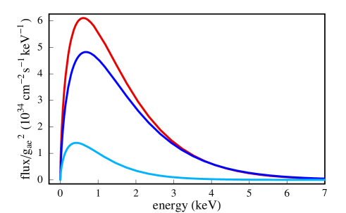
Figure 1: Differential solar axion flux at the Earth, derived by integrating Eq. (1) over SSM [24] up to $r=R_{\odot}$ (red line), $r=0.2\,R_{\odot}$ (blue line), and from $r=0.2\,R_{\odot}$ to $r=R_{\odot}$ (light blue line). The axion-electron coupling $g_{ae}$ is defined in Eq. (4).

In this Letter, we report results of our search for solar hadronic axions which could be produced in the Sun by the bremsstrahlung-like process and detected in the single spectrum of an HPGe detector as the result of the axioelectric effect on germanium atoms. The x rays accompanying the axioelectric effect will be subsequently absorbed in the same crystal, and the energy of the particular outgoing signal equals the total energy of the incoming axion. Because in this experimental set-up the target and detector are the same, the efficiency $\varepsilon$ of the system is substantially increased, i.e., $\varepsilon\approx 1$. The HPGe detector with an active target mass of 1.5 kg was placed at ground level, inside a low-radioactivity iron box with a wall thickness ranging from 16 to 23 cm. The box was lined outside with 1 cm thick lead. The crystal was installed in a standard PopTop detector capsule (Ortec, model CFG/PH4) with a beryllium window of 0.5 mm. The HPGe preamplifier signals were distributed to a spectroscopy amplifier at the 6 $\mu$s shaping time. A low threshold on the output provided the online trigger, ensuring that all the events down to the electronic noise were recorded. The linearity and energy resolution have been studied by using various calibrated sources and, in particular, in the lowest-energy region mainly a ²⁴¹Am source (13.9 keV x-rays and their escape peak of 3.9 keV). Data were accumulated in a 1024-channel analyzer, with an energy dispersion of 63.4 eV/channel, in 20-hour cycles with total time of collection of 275 days. In long-term running conditions, the knowledge of the energy scale is assured by continuously monitoring the positions and resolution of the In x-ray peaks which are present in the measured energy distribution. Drifts were $<\pm 1$ channel and a statistical accuracy of better than 0.6% per channel was attained. Thus, all of the spectra were summed together without applying any gain shifts or offsets and are shown in Fig. 2.

Figure 2: Total measured energy spectrum showing also x-ray peaks from various materials.

Energy resolution (FWHM) was estimated to have a value of 660 eV at the photon energy in the 2.0 - 3.8 keV region, where the axion signal is expected. The former bound is imposed as the analysis threshold due to the electronic noise while the latter one is due to the energy distribution of the solar axions.

Our experiment involves searching for the particular energy spectrum in the measured data,

$$S_{n}=2\,N_{\rm Ge}\,t\int_{E_{n}}^{E_{n+1}}dE^{{}^{\prime}}\int_{0}^{\infty}\frac{d\Phi_{a}}{dE}\sigma_{ae\rightarrow e}\,R(E^{{}^{\prime}},E)dE\>,$$ (5)

produced if the solar axions are detected via axioelectric effect. Here $S_{n}$ is the number of counts detected in detector energy channel $n$, $N_{\rm Ge}$=1.24$\times 10^{25}$ is the number of germanium atoms in our 67 mm in diameter and 80 mm thick HPGe crystal, and $t$ is the time of measurement. Factor 2 is number of electrons in (L₁-) M₁-shell while their binding energies are $E_{\rm b}$(L₁)=1.413 keV and $E_{\rm b}$(M₁)=0.181 keV. The axion response function of the detector $R(E^{{}^{\prime}},E)$ is well represented by a Gaussian (to describe full energy peak) with the amplitude, normalized on the efficiency $\varepsilon$, and width of 0.42 FWHM. Using Eq. (3) from [14], the cross section for axioelectric effect per electron was calculated including contributions from 2$s$ and 3$s$ initial state electrons and may be written in the $m_{a}\rightarrow 0$ & $E\ll m_{e}$ approximation and for $E>E_{\rm b}$(L₁) as:

$$\sigma_{ae\rightarrow e}=\left(\frac{1}{2^{3}}+\frac{1}{3^{3}}\right)\frac{\sqrt{2}}{4\,\pi}\,{g_{ae}^{2}}\,\sigma_{\rm Th}\,{\alpha}^{3}Z^{5}\,\left(\frac{m_{e}}{E}\right)^{3/2}\>.$$ (6)

Here $\sigma_{\rm Th}=6.65\times 10^{-25}$ cm² is the cross section for Thomson scattering, $\alpha$=1/137 is the fine-structure constant, $Z$=32 is the atomic number of Ge, and $m_{e}$ is the electron mass. Equation (6) is consistent with a more general expression $\sigma_{ae\rightarrow e}=(\alpha_{ae}/\alpha)\,(E/2m_{e})^{2}\,\sigma_{\rm ph}$ [27], where $\alpha_{ae}=g_{ae}^{2}/4\,\pi$ and $\sigma_{\rm ph}$ is the photoelectric cross section.

We have used the fit method to analyse the data in order to find upper limits on $g_{ae}$ ($m_{a}$), as described below. Similar approaches have been used by other groups [28] to extract (conservative) upper limits in a case like this where direct background measurement is not possible (the Sun cannot be switched off) and the signal shape is a broad smooth spectrum on top of an unknown background spectrum.

In the fit method we have used the following procedure to make the estimation of an axion signal. The experimental data in the energy interval 2.0 - 3.8 keV (corresponded to MCA channels of 32 to 60) was fitted by the sum of three functions: the electronic noise expectation ($T_{n}$), the background expectation ($B_{n}$) and the effect being searched for ($S_{n}$). To estimate the electronic noise the data were fit to a four-parameter function in the region below 2 keV (corresponded to the channels of 4 to 24); it has the form $T_{n}=A\,n^{B}{\rm exp}(Cn^{D})$, where $A=1.46\times 10^{7}$, $B=6.85$, $C=-0.858$, and $D=1.08$, see Fig. 3 (top panel). As a simple background estimation, suitable for the present purposes, a first-order polynomial $B_{n}=a+bn$ has been assumed. Values of $a=4.54\times 10^{4}$ and $b=-42.5$ were found by fitting $B_{n}$ with the data in the region above 3.8 keV, corresponded to the channels of 70 to 110. From the current limits on the axion mass [17, 18] we estimate that the axion signal is negligible in this channel interval. Contribution of axions was then investigated by extrapolating the electronic noise $T_{n}$ and background $B_{n}$ in the 2.0 - 3.8 keV region, where the detection of axion events should be the most efficient. Inserting Eqs. (3) and (6) in Eq. (5), one can express the expected axion spectrum $S_{n}$ as a function of $g_{ae}^{4}$. As the best values of $A$, $B$, $C$, $D$, $a$ and $b$ had been already determined in the regions where axion contributions could be neglected, only $g_{ae}^{4}$ was varied in the ${\chi}^{2}$ comparison. We were using $g_{ae}^{4}$ instead of $g_{ae}$ as the minimization parameter because the signal strength (i.e., number of counts) is proportional to $g_{ae}^{4}$. The results of the analysis are consistent with $g_{ae}^{4}=(3.6\pm 0.1)\times 10^{-42}$ at 1$\sigma$ level. Figure 3 (bottom panel) displays the results of our fit.

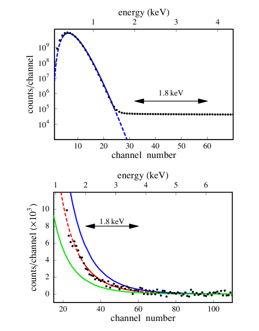
Figure 3: Top panel: low-energy data are shown together with the best fit for the electronic noise expectation $T_{n}$ (solid line) and its extrapolations (dashed line). Bottom panel: residuals from the noise and background expectation are shown together with the expectations for best fit $g_{ae}=4.4\times 10^{-11}$ (red line) as well as for $g_{ae}=5.0\times 10^{-11}$ (blue line) and $g_{ae}=3.7\times 10^{-11}$ (green line). On both panels arrows indicate the energy region of interest for axion signal.

Since we cannot exclude more complicated scenarios in which both the background and the electronic noise modify significantly the energy spectrum of signal events in the region of 32 to 60 channels, we treat the residuals from the noise and background expectation conservatively as an upper limit on the axion signal. In other words, we adopted a criteria commonly used in experiments where direct background measurement is not possible [28] that the theoretically expected signal cannot be larger than that observed at a given confidence level. In this way we obtain the standard 95% C.L. upper limit [2] $g_{ae}\lesssim 4.4\times 10^{-11}$ which translates through Eq. (4) to $m_{a}\lesssim 334$ eV. Because the precise form of the background expectation is not known, we tried also other plausible forms, such as $B_{n}=a+bn+cn^{2}$ and $B_{n}=a+bn+cn^{-1}$. The former yields $g_{ae}^{4}=(2.5\pm 0.2)\times 10^{-42}$ resulting in $m_{a}\lesssim 310$ eV (95% C.L.) while the latter provides $g_{ae}^{4}=(1.4\pm 1.9)\times 10^{-43}$ implying the more stringent limit $m_{a}\lesssim 190$ eV (95% C.L.). One can see that subtraction of the background expectation in a form of $a+bn+cn^{-1}$ cancels the excess of events and the obtained result is very close to the sensitivity of the experiment. Namely, if we assume that the measured spectrum in the region of interest for axion signal is compatible with the background expectation, the fluctuation due to statistical uncertainty imposes a limit on the maximum allowable number of axion events. In this case (the mean is zero and statistical uncertainty for $g_{ae}^{4}$ is $\sigma=2\times 10^{-43}$) we obtain $g_{ae}\lesssim 2.4\times 10^{-11}$ corresponding to $m_{a}\lesssim 170$ eV at the 95% confidence level.

In conclusion, our measurements based on the coupling of the hadronic axions to electrons set a conservative upper limit on the axion mass of $m_{a}\lesssim 334$ eV at 95% confidence level. This upper limit is comparable to the current limits [17, 18] which are extracted from the data taken in the experiments based on the axion-nucleon coupling. We point out the derived limit is free from the large uncertainties and ambiguity, associated with the estimation of the flavor-singlet axial-vector matrix element, which are related to experiments based on the axion-nucleon coupling. New experiments with lower electronic noise and reduced background could improve our search for the hadronic axions. Note that the axioelectric absorption peak in germanium occurs at lower incoming axion momentum when $E$ coincides with the binding energy of atomic shells. At these energies, atomic bound state effects lead to large enhancements in the detection rates of axions, similarly to those in the photoelectric effect. For example, the expected number of axion events for $E>1.4$ keV is about 3 times that for $E>2$ keV. Thus an improvement in the discovery potential may come from examination of the Ge data for energies near the L₁-shell peak of 1.413 keV. Upgradings of the set-up to reduce the electronic noise and permit lowering of the energy threshold below 1 keV are already foreseen and in preparation. In the near future we expect that measurements with the array of 10 - 20 ultra-low-energy IGLET germanium detectors with an anti-Compton shield could improve significantly our understanding on hadronic axions.

We acknowledge support from the Ministry of Science, Education and Sports of Croatia under grant no. 098-0982887-2872.

References

- [1] R.D. Peccei, H.R. Quinn, Phys. Rev. Lett. 38 (1977) 1440.
- [2] W.-M. Yao, et al., Particle Data Group, J. Phys. G 33 (2006) 1, and 2007 partial update for edition 2008 (URL: http://pdg.lbl.gov).
- [3] L. Duffy, et al., Phys. Rev. Lett. 95 (2005) 091304.
- [4] J.E. Kim, Phys. Rev. Lett. 43 (1979) 103; M.A. Shifman, A.I. Vainshtein, V.I. Zakharov, Nucl. Phys. B166 (1980) 493.
- [5] D.B. Kaplan, Nucl. Phys. B260 (1985) 215.
- [6] T. Moroi, H. Murayama, Phys. Lett. B 440 (1998) 69.
- [7] S. Hannestad, A. Mirizzi, G.G. Raffelt, Y.Y.Y. Wong, J. Cosmol. Astropart. Phys. 08 (2007) 015.
- [8] D.M. Lazarus, et al., Phys. Rev. Lett. 69 (1992) 2333; S. Moriyama, et al., Phys. Lett. B 434 (1998) 147. Y. Inoue, et al., Phys. Lett. B 536 (2002) 18; F.T. Avignone III, et al., Phys. Rev. Lett. 81 (1998) 5068. A. Morales, et al., Astropart. Phys. 16 (2002) 325; R. Bernabei, et al., Phys. Lett. B 515 (2001) 6.
- [9] S. Andriamonje, et al., CAST Collaboration, J. Cosmol. Astropart. Phys. 04 (2007) 010.
- [10] G. Raffelt, L. Stodolsky, Phys. Lett. 119B (1982) 323.
- [11] W.C. Haxton, K. Y. Lee, Phys. Rev. Lett. 66 (1991) 2557.
- [12] M. Krčmar, Z. Krečak, M. Stipčević, A. Ljubičić, D.A. Bradley, Phys. Lett. B 442 (1998) 38.
- [13] M. Krčmar, Z. Krečak, M. Stipčević, A. Ljubičić, D.A. Bradley, Phys. Rev. D 64 (2001) 115016.
- [14] A. Ljubičić, D. Kekez, Z. Krečak, T. Ljubičić, Phys. Lett. B 599 (2004) 143.
- [15] K. Jakovčić, Z. Krečak, M. Krčmar, A. Ljubičić, Radiat. Phys. Chem. 71 (2004) 793.
- [16] A.V. Derbin, A.I. Egorov, I.A. Mitropol´sky, V.N. Muratova, JETP Lett. 81 (2005) 365.
- [17] T. Namba, Phys. Lett. B 645 (2007) 398.
- [18] A.V. Derbin, et al., JETP Lett. 85 (2007) 12.
- [19] P. Belli, et al., Nucl. Phys. A 806 (2008) 388.
- [20] E. Leader, A.V. Sidorov, D.B. Stamenov, JHEP 0506 (2005) 033.
- [21] M. Srednicki, Nucl. Phys. B260 (1985) 689.
- [22] G. G. Raffelt, Phys. Rev. D 33 (1986) 897.
- [23] A.R. Zhitnitsky, Yu.I. Skovpen, Sov. J. Nucl. Phys. 29 (1979) 513, Yad. Fiz. 29 (1979) 995 (in Russian).
- [24] J.N. Bachall, A.M. Serenelli, S. Basu, Astrophys. J. 621 (2005) L85, (URL:http://www.sns.ias.edu/jnb/).
- [25] G. Raffelt, Stars as Laboratories for Fundamental Physics (Chicago Univ. Press, Chicago, 1996); G.G. Raffelt, D.S.P. Dearborn, Phys. Rev. D 36 (1987) 2211.
- [26] H. Schlattl, A. Weiss, G. Raffelt, Astropart. Phys. 10 (1999) 353.
- [27] S. Dimopoulos, G.D. Starkman, B.W. Lynn, Mod. Phys. Lett. A 1 (1986) 491.
- [28] See for instance: E. García, et al., Phys. Rev. D 51 (1995) 1458; L. Baudis, et al., HDMS, Phys. Rev. D 59 (1998) 022001; A. Morales, et al., IGEX, Phys. Lett. B 532 (2002) 8; G. Angloher, et al., CRESST, Astropart. Phys. 18 (2002) 43; J. Angle, et al., XENON, Phys. Rev. Lett. 100 (2008) 021303.