Coherent-incoherent transition in a Cooper-pair-box coupled to a quantum oscillator: an equilibrium approach

Abstract

Temperature effect on quantum tunneling in a Cooper-pair-box coupled to a quantum oscillator is studied by both numerical and analytical calculations. It is found that, in strong coupling regions, coherent tunneling of a Cooper-pair-box can be destroyed by its coupling to a quantum oscillator and the tunneling becomes thermally activated as the temperature rises, leading to failure of the Cooper-pair-box. The transition temperature between the coherent tunneling and thermo-activated hopping is determined and physics analysis based on small polaron theory is also provided.

I Introduction

Since the experimental realization of the single-electron transistor (SET) in 1987,al ; fd the SET has become an important element in both extremely precise measurementbw ; zb ; kc ; la and quantum information processing.aa ; mss ; dv The development of the so-called radio-frequency SET electrometer is considered as the electrostatic “dual” of the well known superconducting quantum interference devices (SQUIDs) and has shown its power of fast and ultrasensitive measurement.sch ; sch1 On the other hand, the direct observation of the coherent oscillation in superconducting SET (SSET, or the so-called Cooper-pair-box (CPB)) shows the SSET can be served as a physical realization of a coherent two-state system,na ; na1 and since then the SSET or the SSET-based circuit has been considered as a candidate of a qubit in a solid state device and a read-out device of a qubit.aa ; mss ; dv

The high frequency (up to 1 GHz) and high quality factor ($Q\sim 10^{3}$) nano-mechanical resonator (NR) was firstly fabricated from bulk silicon crystal in 1996,cr and therefore it brought a lot of interest in demonstrating the quantum nature of this small mechanical device.is ; ir ; lt ; ts ; ar A nano-mechanical resonator capacitively coupled to a SSET forms the so-called nano-electromechanical system (NEMS), a system shows promises for fast and ultrasensitive force microscopy.la ; pb Especially, displacement-detection approaching the quantum limit by this system has been demonstrated.la From a view point of theoretical study, NEMS can be interesting in their own right. In fact, NEMS provides a physical realization of a simple quantum system: a two-level system (TLS) coupled to a single phonon mode, which has basic relation to some important models in solid state physics and quantum optics. First of all, it represents an oversimplified spin-boson model,leg ; weiss i.e., the spin-boson model in a single-phonon mode case, also it can be considered as the Einstein model in a two-site problem in the exciton-phonon (or polaron-phonon) system.ss By taking the analog of the resonator as the single mode cavity, it is the Jaynes-Cummings model in quantum optics.lt ; jm ; jc ; sun

To be a physical realization of a TLS, the SSET needs to work in severe constrains. It is well known that both thermal and quantum fluctuations from the environment can destroy the Coulomb blockade of tunneling and lead to the failure of the SET.al1 ; hd Additional conditions are needed for a SSET,al1 and one important factor is to maintain the coherent tunneling. The study on polaron-phonon system shown that the coherent motion of the electron can be destroyed by its coupling to the phonon and a transition from band motion to hopping motion happens as the temperature rises.mah By analogy, it is important to know if the coherent tunneling of the SSET in NEMS can be destroyed by its coupling to a NR, leading to failure of the SSET. We shall state such a phonon-induced transition as coherent-incoherent transition and this is the main interest of the present paper.

The coherent-incoherent transition in NEMS will be studied by both numerical and analytical analyses. It is shown that the coherent-incoherent transition exists for some frequency ranges with strong coupling parameters. The rest of the present paper is organized as follows. In Sec. II, we explain the model and the way to trace out the environment, the results from adiabatic approximation is also discussed. The coherent-incoherent transition is studied in Sec. III and conclusion and discussion are presented in Sec. IV.

II The model and explanation of the approximation

The Hamiltonian of the NEMS, i.e., a TLS $+$ a NR, is given by (setting $\hbar=1$)mss ; ar

$$\hat{H}_{0}=\frac{1}{2}\epsilon_{0}\hat{\sigma}_{z}-\frac{1}{2}\Delta_{0}\hat{\sigma}_{x}+\Omega\hat{a}^{\dagger}\hat{a}+\lambda\hat{\sigma}_{z}(\hat{a}^{\dagger}+\hat{a}),$$ (1)

where $\epsilon_{0}=E_{C}(1-2n_{g})$ and $E_{C}$ is the charging energy of a Cooper pair, $n_{g}=C_{g}V_{g}/(2e)$ with $C_{g}$ and $V_{g}$ are the gate capacity and gate voltage, respectively. $\Delta_{0}=E_{J}=I_{c}/(2e)$ and $I_{c}$ is the critical current of the Josephson junction. $\hat{\sigma}_{i}$ ($i=x,y,z$) are the Pauli matrices and $\hat{a}^{\dagger}$ $(\hat{a})$ is the creation (annihilation) operator of the phonon mode with energy $\Omega$, while $\lambda$ is the coupling parameter. The above Hamiltonian indicates that our main interest is the case when the SSET is closed to the degeneracy point.mss ; ar It should be noted that the system described by the above Hamiltonian is not a thermodynamical system, a true thermodynamical system should include the environment, which is modeled as a collection of harmonic oscillators.leg ; weiss The whole Hamiltonian can be written as

$$\hat{H}=\hat{H}_{0}+\hat{H}_{e},\quad\hat{H}_{e}=\sum_{k}\omega_{k}\hat{b}_{k}^{\dagger}\hat{b}_{k}+\hat{H}_{int},$$ (2)

where $\hat{H}_{int}$ represents the coupling between the environment and NEMS. In the present paper, we shall assume that the effect of the environment is just to keep the NEMS in equilibrium. Here we apply the concept of reduced density matrix to explain the approximation. The density matrix of the whole system is

$$\rho=\rho_{0}\otimes\rho_{e},$$ (3)

where $\rho_{0}$ and $\rho_{e}$ are the density matrix of the NEMS and environment, respectively. The expectation value of any operator $\hat{Q}$ that acts only on the variables of the NEMS can be found bybl

$$\langle\hat{Q}\rangle={\rm Tr}\rho_{r}(\phi)\langle\phi|\hat{Q}|\phi\rangle,\quad\rho_{r}={\rm Tr}_{bath}\rho,$$ (4)

where $\rho_{r}$ is the reduced density matrix and “${\rm Tr}_{bath}$” means the trace operation over the environment. Our approximation means that the above expression can be rewritten as

$$\langle\hat{Q}\rangle\simeq\frac{1}{Z}\sum_{i}e^{-\beta E_{i}}\langle\phi_{i}|\hat{Q}|\phi_{i}\rangle,~{}~{}~{}~{}~{}~{}~{}~{}\hat{H}_{0}|\phi_{i}\rangle=E_{i}|\phi_{i}\rangle,$$ (5)

with $Z=\sum_{i}e^{-\beta E_{i}}$ is the partition function of the NEMS and $\beta=1/T$ (setting $k_{B}=1$). In previous treatments,ir ; lt the effect of the environment is just to keep the NR in equilibrium. The present treatment, taking a small step further, suggests that the NEMS is in equilibrium with the environmental bath.

By taking this approximation, thermodynamical properties of the NEMS can be known, provided that the eigenvalue problem of $\hat{H}_{0}$ in Eq. (1) can be solved. The eigenvalues of $\hat{H}_{0}$ can be obtain by the standard numerical diagonalization technique. In a practical treatment, the number of eigenvalues treated must be finite, we therefore truncate the eigenspectrum by just taking the first smallest $N$ eigenvalues, i.e.,

$$\langle\hat{Q}\rangle\simeq\frac{1}{Z}\sum_{i}e^{-\beta E_{i}}\langle\phi_{i}|\hat{Q}|\phi_{i}\rangle\simeq\frac{1}{Z}\sum_{i=1}^{N}e^{-\beta E_{i}}\langle\phi_{i}|\hat{Q}|\phi_{i}\rangle,$$ (6)

with $Z\simeq\sum_{i=1}^{N}e^{-\beta E_{i}}$, while $N$ is determined by the following condition

$$\beta(E_{N}-E_{1})\geq L,$$ (7)

where $L$ is a fixed number to control the calculation error and in the present paper we have $L\geq 20$. Accordingly, one can find the interested physical quantities from the numerical results, for example, the free energy of the NEMS is

$$F(T)\simeq-T\ln\left(\sum_{i=1}^{N}e^{-\beta E_{i}}\right),$$ (8)

from which all the thermodynamical quantities of the NEMS can be found. In our numerical calculation, we have randomly checked the dependence of the results on the value of $L$. We found no observable dependence on $L$ for $L\geq 20$ by extending $L$ to 50 or even 100. It should be noted that, for calculating the temperature dependence of tunneling splitting, Eq. (5) should be modified as

$$\Delta(T)\simeq\frac{1}{Z}\sum_{i=1}^{N}e^{-\beta E_{i}}|\langle\phi_{i}|\hat{\sigma}_{x}|\phi_{i}\rangle|,$$ (9)

this is because the sign of $\langle\phi_{i}|\hat{\sigma}_{x}|\phi_{i}\rangle$ is not relevant in the calculation of $\Delta(T)$.

Before going to numerical results, we shall first discuss the adiabatic approximation in the case of $\epsilon_{0}=0$ which was shown to be a good approximation for $\Delta_{0}/\Omega\leq 1$.ir In the adiabatic approximation, the eigenvalues of $\hat{H}_{0}$ are characterized by pairs of energies that are given byir

$$E_{a}^{\pm}(n)=n\Omega\pm\Delta_{a}(n)-\frac{\lambda^{2}}{\Omega},\quad\Delta_{a}(n)=\frac{\Delta_{0}}{2}\langle n_{+}|n_{-}\rangle,$$ (10)

where $|n_{\pm}\rangle=\exp\{\mp(\lambda/\Omega)(a^{+}-a)\}|n\rangle$ are the displaced-oscillator states and $n=0,1,2,\cdots$. Taking these eigenvalues, one can find the temperature dependence of the tunneling splitting according to Eq. (9) and the result is

$$\Delta_{a}(T)\simeq\frac{1}{Z_{a}}\sum_{n=0}^{\infty}\Delta_{a}(n)e^{-\beta n\Omega}~{}2\cosh(\beta\Delta_{a}(n)),$$ (11)

where $Z_{a}=\sum_{n=0}^{\infty}e^{-\beta n\Omega}~{}2\cosh(\beta\Delta_{a}(n))$. In the limit of $\Delta_{a}(n)\ll\Omega$, it can be found that

$$\Delta_{a}(T)\simeq\sum_{n=0}^{\infty}\Delta_{a}(n)p_{{\rm th}}(n),~{}~{}~{}~{}~{}~{}p_{{\rm th}}(n)=e^{-\beta n\Omega}(1-e^{-\beta\Omega}),$$ (12)

a result that was used in the previous treatments.ir ; lt

III Coherent-incoherent transition

To perform numerical diagonalization, one needs to represent the Hamiltonian $\hat{H}_{0}$ with a suitable basis. In the treatment of Ref. ir, , the basis of $|\uparrow,\downarrow\rangle\otimes|n_{\pm}\rangle$ is applied, where $|\uparrow\rangle$ and $|\downarrow\rangle$ are the eigenstates of $\sigma_{z}$. However, with this basis, the elements of the Hamiltonian matrix are flooded with the overlap terms between different states $|n_{\pm}\rangle$ as shown in the Eq. (8) of Ref. ir, . Such overlap terms are rather complicated to compute and therefore the generation of the Hamiltonian matrix will be slow. In our treatment, for convenient, we use a very simple basis that consist of the eigenstates of $\sigma_{z}$ and $\hat{a}^{\dagger}\hat{a}$ to represent the Hamiltonian, i.e., a basis of $|\uparrow,\downarrow\rangle\otimes|n\rangle$. Hence, we represent the TLS terms with $|\uparrow,\downarrow\rangle$ and the NR terms with $|n\rangle$ and do a tensor product, the matrix of $\hat{H}_{0}$ is generated. Of course, both schemes give the same results. The diagonalization can give the eigenvalues of $\hat{H}_{0}$, i.e., $\{E_{i}\}$, and the corresponding eigenvectors $\{\phi_{i}\}$, from which the tunneling splitting $\langle\phi_{i}|\hat{\sigma}_{x}|\phi_{i}\rangle$ can be found. Noted that, to reach the accuracy condition (7), the matrix size is $\Omega$-dependent, the lower the frequency, the larger the matrix size. In the following, we shall firstly concentrate our interest on the unbiased case of $\epsilon_{0}=0$ and the biased case will be discussed in the end of this section. The eigenvalues in the case of $\epsilon_{0}=0$ we found are in good agreement with the results in Ref. ir, , i.e., the results of the adiabatic approximation given in Eq. (10) work well for $\Omega/\Delta_{0}\geq 1$. The corresponding tunneling splitting of the eigenstates for $\lambda/\Omega=0.5$ and some typical values of $\Delta_{0}/\Omega$ are shown in Fig. 1, where the results of the adiabatic approximation are also given for comparison.

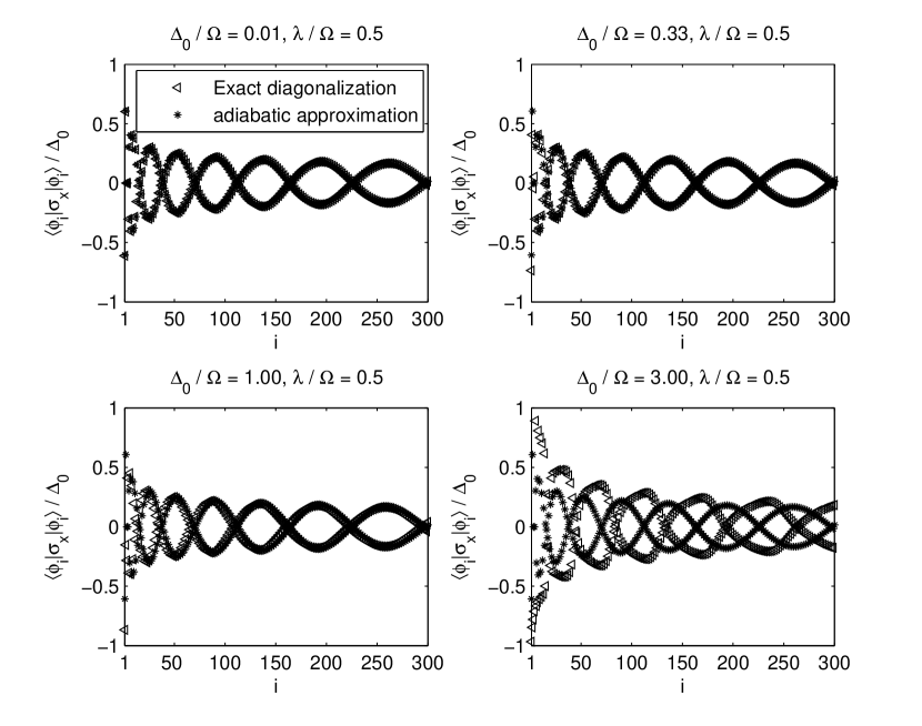
Figure 1: Tunneling splitting for eigenstates of $\hat{H}_{0}$ in the case of $\lambda/\Omega=0.5$ and $\epsilon_{0}=0$ for some typical values of $\Delta_{0}/\Omega$ by numerical calculation (shown as triangles). The results of the adiabatic approximation (shown as “$\ast$”) are also shown for comparison. The sketches of both curves show good agreement for $\Delta_{0}/\Omega\leq 1$ and the higher the excited states the better the agreement. However, obvious discrepancy appears for both the ground state and the first excited state even when $\Delta_{0}/\Omega=1/3$. The results of the adiabatic approximation show large discrepancy with the numerical results in low frequency region with $\Delta_{0}/\Omega>1$.

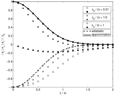
Figure 2: Comparison of the tunneling splitting of both the ground state and the first excited state by numerical calculation with adiabatic approximation in the case of $\epsilon_{0}=0$ for some typical values of $\Delta_{0}/\Omega$. It should be noted that the result by adiabatic approximation is $\Delta_{0}/\Omega$-independent, which is shown as solid and dash lines (dash line is the ground state). Numerical results are shown in different patterns for different values of $\Delta_{0}/\Omega$ (the hollow patterns are for the ground state).

It can be found that the sketches of both curves show good agreement for $\Delta_{0}/\Omega\leq 1$ and the higher the excited states the better the agreement. However, a closed look at the curves shows that obvious discrepancy appears for both the ground state and the first excited state even when $\Delta_{0}/\Omega=1/3$. Figure 2 shows the details of the discrepancy. We found that the discrepancy begins to appear even when $\Delta_{0}/\Omega=0.1$ and becomes obvious when $\Delta_{0}/\Omega=1/3$. The present results show that, if one compares the eigenvalues of the adiabatic approximation with the numerical diagonalization, the adiabatic approximation seems to work pretty well for $\Delta_{0}/\Omega\leq 1$; however, if one measures the tunneling splitting, the adiabatic approximation works well only for $\Delta_{0}/\Omega\leq 0.1$.

After finding out the eigenvalues and the corresponding tunneling splitting, one can calculate temperature dependence of the tunneling splitting according to Eq. (8). For all the frequencies we studied (down to $\Delta_{0}/\Omega=50$), it is found that the tunneling splitting decreases with temperature at the beginning in low temperature regions. However, when the coupling strength $\lambda/\Omega$ increases to some critical value, $\Delta(T)$ has a “upturn” at some temperature $T_{t}$, which is $\lambda/\Omega$-dependent. Typical results are shown in Fig. 3.

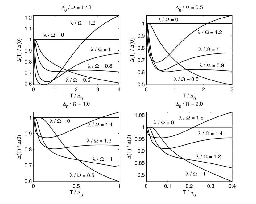
Figure 3: Temperature dependence on the tunneling splitting in the case of $\epsilon_{0}=0$ for some typical values of $\Delta_{0}/\Omega$. At the beginning, $\Delta(T)$ decreases with temperature, but as the coupling parameter $\lambda/\Omega$ increases, $\Delta(T)$ shows a “up-turn” at some temperature $T_{t}$, which is $\lambda/\Omega$-dependent.

The curves shown in Fig. 3 indicate that, for a given value of $\Delta_{0}/\Omega$ and in the low temperature region, the main effect of the NR on quantum tunneling is to decreases the tunneling splitting in the weak coupling regions. The situation is more or less the same as that in the polaron-phonon (or exciton-phonon) system, say, coupling to phonons makes the electron become a “dressed” one and lowers the hopping rate of the electron. However, as the coupling strength increases, the effect of the NR on quantum tunneling changes as temperature increases to $T_{t}$, e.g., the tunneling splitting is enhanced by a NR as temperature increases further. The result is reminiscent of the transition from Bloch-type band motion to phonon-activated hopping motion in the polaron-phonon (or exciton-phonon) system.mah Moreover, $\Delta_{a}(T)$ obtained from Eq. (11) does not show such “upturn” for the frequency regions we studied. This implies that the “up-turn” is a non-adiabatic effect.

As we have mentioned in Sec. I, the present model can be considered as an analog to the polaron-phonon system of Einstein model.mah We therefore employ the small polaron theory to analyze the temperature dependence of the tunneling splitting. At the beginning of the low temperature regions, the expectation value of phonon number is small, the main contribution to the tunneling splitting is the so-called diagonal transitions. The diagonal transition rate can be found by following the way given in Ref. mah, . Firstly, a canonical transformation is applied to the Hamiltonian in Eq.(2), i.e.,

$$\hat{H}^{\prime}=e^{S}\hat{H}e^{-S}=\hat{{\cal H}}_{0}+\hat{V}+\sum_{k}\omega_{k}\hat{b}_{k}^{\dagger}\hat{b}_{k}+\hat{H}_{int}^{\prime},$$ (13)

where $S=(\lambda/\Omega)\hat{\sigma}_{z}(\hat{a}^{\dagger}-\hat{a})$,

$$\hat{{\cal H}}_{0}=\frac{\epsilon_{0}}{2}\hat{\sigma}_{z}+\Omega\hat{a}^{\dagger}\hat{a}-\frac{\lambda^{2}}{\Omega},$$ (14)

$$\hat{V}=\frac{\Delta_{0}}{4}(\hat{\sigma}_{+}e^{(\lambda/\Omega)(\hat{a}-\hat{a}^{\dagger})}+h.c.),$$ (15)

$\hat{H}_{int}^{\prime}=e^{S}\hat{H}_{int}e^{-S}$ and $\hat{\sigma}_{\pm}=\hat{\sigma}_{x}\pm i\hat{\sigma}_{y}$. The diagonal transition rate is given by

$$w_{d}(T)={\rm Tr}_{\hat{{\cal H}}_{0}}\langle i|\hat{V}|i\rangle=\frac{\Delta_{0}}{2}e^{-S_{T}},$$ (16)

where $S_{T}=(2\lambda/\Omega)^{2}(n+1/2)$ and $n=(e^{\beta\Omega}-1)^{-1}$ is the expectation value of phonon number. Here, we have employed the approximation elucidated in Sec. II, i.e., the effect of $\sum_{k}\omega_{k}\hat{b}_{k}^{\dagger}\hat{b}_{k}+\hat{H}_{int}^{\prime}$ is just to keep the NEMS in equilibrium. $w_{d}$ and hence the tunneling splitting will decrease with increasing temperature. On the other hand, the main contribution to tunneling splitting, at higher temperature, is the so-called non-diagonal transitions. One can calculate the correlation function in the way given in Ref. mah, , e.g.,

$$W(t)={\rm Tr}_{\hat{{\cal H}}_{0}}[\langle i|\hat{V}(t)\hat{V}(0)|i\rangle-|\langle i|\hat{V}|i\rangle|^{2}],$$ (17)

with $\hat{V}(t)=e^{i\hat{{\cal H}}_{0}t}\hat{V}e^{-i\hat{{\cal H}}_{0}t}$ and the result is

$$W(t)=(\Delta_{0}/2)^{2}e^{-2S_{T}}[e^{\varphi(t)}-I_{0}(\epsilon)],$$ (18)

where $I_{0}(x)$ is a Bessel function and

$$\varphi(t)=\epsilon\cos[\Omega(t+i\beta\hbar/2)],\quad\epsilon=2(2\lambda/\Omega)^{2}[n(n+1)]^{1/2}.$$ (19)

It is interesting to note that, in the present case, the factor $I_{0}(\epsilon)$ still survives after taking thermodynamical limit, a situation that is different from the small polaron theory of the Einstein model.mah This is because only one phonon mode coupled to the TLS in the present case and all the other modes just serve as the bath. This result can also help to get rid of the delta function problem shown in Ref. mah, . The non-diagonal transition rate can be found by using the saddle-point integration

$$w_{n}(T)=\int_{-\infty}^{\infty}W(t)dt\simeq(\Delta_{0}/2)^{2}(\pi/\gamma)^{1/2}e^{-2S_{T}+\epsilon},$$ (20)

where $\gamma=\lambda^{2}[n(n+1)]^{1/2}$. It can be easily checked that $w_{n}$ shows opposite temperature dependence to $w_{d}$ and the transition temperature $T_{t}$ is determined by $w_{d}=w_{n}$, which leads to

$$\frac{\Delta_{0}}{2}[\pi/\gamma(T_{t})]^{1/2}e^{\epsilon(T_{t})-S_{T}(T_{t})}=1.$$ (21)

The above equation can be solved numerically and the transition temperatures obtained are shown in Fig. 4, where the transition temperatures determined from $\Delta(T)$ by numerical calculation (i.e., curves shown in Fig. 3) are also presented for comparison.

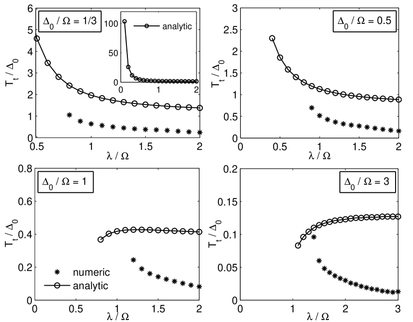
Figure 4: Transition temperatures obtained by analytical (from Eq.(21)) and numerical calculations in the case of $\epsilon_{0}=0$ for some typical values of $\Delta_{0}/\Omega$. The analytical results are always higher than the numerical ones. For $\Delta_{0}/\Omega<1$, both transition temperatures show similar $\lambda/\Omega$ dependence, i.e., $T_{t}$ decreases with increasing $\lambda/\Omega$. However, opposite $\lambda/\Omega$ dependence is found for $\lambda/\Omega\geq 1$, showing that the analytical results are invalid in the low frequency regions. The inset of the lefttop figure shows the whole transition temperature curve obtained by the analytical calculation.

It can be seen from Fig. 4 that the transition temperatures from numerical calculations are always lower than the analytical ones. In high frequency region with $\Delta_{0}/\Omega<1$, both obtained transition temperatures show similar $\lambda/\Omega$ dependence, i.e., $T_{t}$ increases as $\lambda/\Omega$ decreases. However, the transition temperature obtained from analytical calculation shows opposite coupling parameter dependence in low frequency region with $\Delta_{0}/\Omega<1$, a result that is in confliction with an intuitive picture. We notice that, as shown in the inset of Fig. 4, analytical calculation predicts a transition for coupling strength as low as $\lambda/\Omega\sim 0.2$ for $\Delta_{0}/\Omega\leq 1/3$; however, numerical result shows that there is no transitions for coupling strength $\lambda/\Omega$ lower than 0.7. Figure 5 draws the the transition boundary as a function of $\lambda/\Omega$ and $\Delta_{0}/\Omega$ obtained by the numerical calculation.

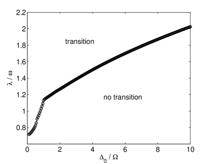
Figure 5: Transition boundary obtained by the numerical calculation in the case of $\epsilon_{0}=0$. The larger the $\Delta_{0}/\Omega$ (i.e., the lower frequency for a given $\Delta_{0}$), the larger the coupling strength $\lambda/\Omega$ is needed for the transition to happens, indicating the SSET is more stable when coupling to a lower frequency NR.

We believe that the discrepancy mainly comes from the approximation made in the analytical calculation of the diagonal transition rate. It can be shown that

$$w_{d}(T)=\sum_{n=0}^{\infty}\Delta_{a}(n)p_{{\rm th}}(n)\simeq\Delta_{a}(T),$$ (22)

which indicates that effectively the diagonal transition rate is found by adiabatic approximation, an approximation is good for finding the tunneling splitting only when $\Delta_{0}/\Omega\leq 0.1$. Figure 6 shows the details of how the discrepancy comes from the adiabatic approximation.

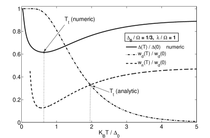
Figure 6: Illustration of how the discrepancy comes from $w_{d}(T)$ obtained by the adiabatic approximation in the case of $\epsilon_{0}=0$, $\Delta_{0}/\Omega=1/3$, and $\lambda/\Omega=1$. As the temperature increases, the descending rate of $w_{d}(T)/w_{d}(0)$ is much lower than $\Delta(T)/\Delta(0)$ from the numerical calculation, leading to a higher transition temperature. The “up-turn” of $w_{n}(T)$ in the low temperature regions is due to the factor $\gamma^{-1/2}$ which diverges as $T\rightarrow 0$.

It turns out that, as the temperature increases, the descending rate of $w_{d}(T)/w_{d}(0)$ is much lower than $\Delta(T)/\Delta(0)$ from the numerical calculation. Such a result has two consequences. The first one is the transition temperature by analytical calculation is higher than the numerical result since a slower descending $w_{d}(T)/w_{d}(0)$ will lead to a higher crosspoint with a given $w_{n}(T)$; Still another is the extremely high transition temperature in the weak coupling regions shown in the inset of Fig. 4. It is found that, in the weak coupling regions, the slow descending $w_{d}(T)/w_{d}(0)$ can still survive to some high temperature, at where $\Delta(T)$ from the numerical calculation has died out, bringing about an artifact high transition temperature. On the other hand, As one can see from Fig. 1 and Fig. 2, tunneling splitting from the adiabatic approximation shows large discrepancy with the numerical result when $\Delta_{0}/\Omega\geq 1$. This implies that $w_{d}(T)$ is a bad approximation to calculate the diagonal transition rate in low frequency regions with $\Delta_{0}/\Omega\geq 1$. Numerical analysis indicates that $w_{d}(T)$ shows different $(\lambda/\Omega)$-dependence from $\Delta(T)$, leading to different $\lambda/\Omega$-dependence of $T_{t}$. In other words, the break-down of the adiabatic approximation in the low frequency region with $\Delta_{0}/\Omega\geq 1$ leads to an abnormal $\lambda/\Omega$-dependence of the transition temperature in the low frequency regions.

Now we turn to see the effect of bias on the coherent-incoherent transition. In the case of $\epsilon_{0}\not=0$, intuitively, the hopping between the TLS needs the assistance of the phonon unless the bias is very small comparing with $\Delta_{0}$, i.e., the bias can be overcome by the quantum fluctuation. Accordingly, the diagonal transition is still possible and hence the coherent-incoherent transition is expected to survive only when $\epsilon_{0}/\Delta_{0}\ll 1$. Nevertheless, the appearance of the non-zero bias will weaken the diagonal transition rate. As $\epsilon_{0}$ increases to some value, at where tunneling becomes impossible without the assistance of phonon, then the diagonal transition makes no contribution to tunneling and coherent-incoherent transition disappears. Numerical calculation in the case of $\epsilon_{0}\not=0$ is the same as $\epsilon_{0}=0$ and some typical results obtained by the numerical calculation are shown in Fig. 7. As $\epsilon_{0}/\Delta_{0}$ increases, the transition temperature decreases and the transition disappears when $\epsilon_{0}/\Delta_{0}$ reaches some critical value which is a function of $\lambda/\Omega$ and $\epsilon_{0}/\Omega$. Obviously, the numerical result is in accord with the analysis presented above.

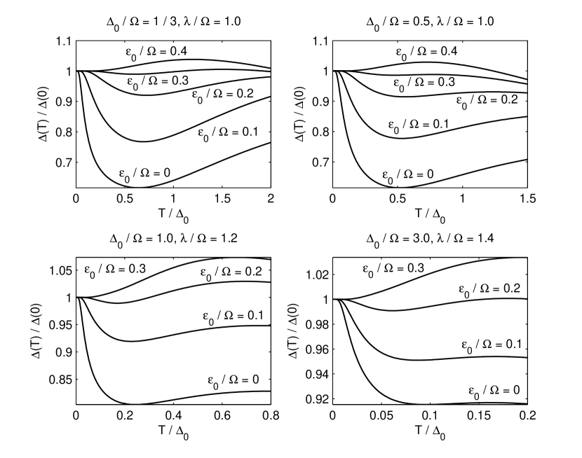
Figure 7: The effect of bias on the coherent-incoherent transition for some typical values of $\lambda/\Omega$ and $\Delta_{0}/\Omega$. The transition temperature decreases with increasing $\epsilon_{0}/\Omega$ and the transition disappears when $\epsilon_{0}/\Omega$ reaches some critical value which depends on both $\lambda/\Omega$ and $\Delta_{0}/\Omega$.

IV Conclusion and discussion

In conclusion, we have presented study on the effect of a nanomechanical resonator on quantum tunneling in a Cooper-pair-box at $T\not=0$. We found that the coherent tunneling of a Cooper-pair-box can be destroyed by the coupling to a NR at a temperature much lower than the coupling energy $E_{J}$ of the Josephson junction. The present analysis shows that, for a NEMS to work well, one additional condition, e.g., $T\ll T_{t}$, is needed. The coherent-incoherent transition boundary as a function of $\Delta_{0}/\Omega$ and $\lambda/\Omega$ is calculated. It turns out that the transition happens only for $\lambda/\Omega>0.7$, and the lower the $\Delta_{0}/\Omega$, the larger the $\lambda/\Omega$ is needed for the transition. We also found that the transition temperature is a monotonic descending function of $\lambda/\Omega$. The present result shows that experimental observation on the coherent-incoherent transition is still impossible since the corresponding coupling parameter cannot be achieved in the present stage. Taking some typical experimental parameters:is $\Delta_{0}=4\mu$eV and $\hbar\Omega=1.2\mu$eV, the coupling parameter needed for the transition is $\lambda/\Omega\simeq 1.4$, which is larger than the strong coupling limit possible to achieve in experiment $(\lambda/\hbar\omega_{0}\sim 1)$.ir To see the transition in the coupling parameters can be achieved in experiment, the result shown in Fig. 5 tells $\Delta_{0}/\Omega$ should lower than 1, i.e., the frequency of the NR should be as high as 1GHz, which is almost the limitation in the present stage. Nevertheless, it is believed that, in a real system, the transition can be seen in a lower coupling parameter regions since the coupling of the NR to the environment can help the transition to happen. It is also found that other thermodynamical quantities, like specific heat, vary smoothly over the transition point, showing that the transition is not a thermodynamical transition.

Coherent-incoherent transition is an important issue in the spin-boson model and analysis on the transition at $T\not=0$ was also provided in Ref. leg, . However, the starting point in Ref. leg, is different from the present analysis. In the present analysis, the key element is the temperature dependence on the tunneling splitting, while in the previous analysis, it is the relaxation behavior, i.e., the time dependence on transition rate $P(t)$.leg As a matter of fact, the present analytic calculation is similar to the calculation provided in Sec. III D of Ref. leg, , and accordingly the transition rate we found here is corresponding to $\Gamma$ (or $1/(2\tau)$), which was predicted to have a monotonic temperature dependence in their analysis. It seems that this result is suitable for the case with large bias while the “up-turn” of $\Delta(T)$ for small (or zero) bias cannot be explained. Nevertheless, the present result can help to understand the coherent-incoherent transition at $T\not=0$ in the spin-boson model with small bias. To the first order approximation (i.e., omitting the cooperative effect between different phonon modes), the combined contribution of all the phonon modes with a frequency-dependent weight for $0<\omega<\omega_{c}$ is approximately the contribution of the whole bath, accordingly a coherent-incoherent transition is expected to exist in the spin-boson model since the coupling of the TLS to all the phonon modes can lead to the transition when the coupling strength exceeds some value.

- (1) D. V. Averin and K. K. Likharev, J. Low Temp. Phys. 62, 345 (1986).
- (2) T. A. Fulton and G. J. Dolan, Phys. Rev. Lett. 59, 109 (1987).
- (3) M.P. Blencowe, M.N. Wybourne, Appl. Phys. Lett. 77, 3845 (2000).
- (4) Y. Zhang and M.P. Blencowe, J. Appl. Phys. 91, 4249 (2002).
- (5) R. G. Knobel, A. N. Cleland, Nature (London) 424, 291 (2003).
- (6) M. D. LaHaye, O. Buu, B. Camarota, and K. C. Schwab, Science 304, 74 (2004).
- (7) A. Aassime, G. Johansson, G. Wendin, R. J. Schoelkopf, and P. Delsing, Phys. Rev. Lett. 86, 3376 (2001).
- (8) Y. Makhlin, G. Schön, and A. Shnirman, Rev. Mod. Phys. 73, 357 (2001).
- (9) D. Vion, A. Aassime, A. Cottet, P. Joyez, H. Pothier, C. Urbina, D. Esteve, and M. H. Devoret, Science 296, 886 (2002).
- (10) R. J. Schoelkopf, P. Wahlgren, A. A. Kozhevnikov, P. Delsing, and D. E. Prober, Science 280, 1238 (1998).
- (11) M. H. Devoret and R. J. Schoelkopf, Nature (London) 406, 1039 (2000).
- (12) Y. Nakamura, C. D. Chen, and J. S. Tsai, Phys. Rev. Lett. 79, 2328 (1997).
- (13) Y. Nakamura, Yu. A. Pashkin, and J. S. Tsai, Nature (London), 398, 786 (1999).
- (14) A. N. Cleland and M. L. Roukes, Appl. Phys. Lett. 69, 2653(1996); Nature (London), 392, 160 (1998).
- (15) E. K. Irish and K. Schwab, Phys. Rev. B 68, 155311 (2003).
- (16) E. K. Irish, J. Gea-Banacloche, I. Martin, and K. C. Schwab, Phys. Rev. B 72, 195410 (2005).
- (17) L. Tian, Phys. Rev. B 72, 195411 (2005).
- (18) T. Sandu, Phys. Rev. B 74, 113405 (2006).
- (19) A. D. Armour, M. P. Blencowe, and K. C. Schwab, Phys. Rev. Lett. 88, 148301 (2002).
- (20) M. P. Blencowe, Contemp. Phys., 46, 249 (2005).
- (21) A. J. Leggett, S. Chakravarty, A. T. Dorsey, M. P. A. Fisher, A. Garg, and W. Zwerger, Rev. Mod. Phys. 59, 1 (1987) and references there in.
- (22) U. Weiss, Quantum Dissipative Systems, (World Scientific, Singapore, 1999).
- (23) H. B. Shore and L. M. Sander, Phys. Rev. B 7, 4537 (1973).
- (24) J. M. Raimond, M. Brune, and S. Haroche, Rev. Mod. Phys. 73, 565 (2001).
- (25) E. T. Jaynes and F. W. Cummings, Proc. IEEE 51, 89 (1963).
- (26) F. Xue, L. Zhong, Y. Li, and C. P. Sun, Phys. Rev. B 75, 033407 (2007).
- (27) D. V. Averin and K. K. Likharev, in Mesoscopic Phenomena in Solids, ed. by B. L. Altshuler, P. A. Lee, and R. A. Webb, (North-Holland, Amsterdam, 1991).
- (28) M. H. Devoret, D. Esteve, H. Grabert, G.-L. Ingold, H. Pothier, and C. Urbina, Phys. Rev. Lett. 64, 1824 (1990).
- (29) G. D. Mahan, Many-Particle Physics, (Plenum Press, New York, 1990).
- (30) K. Blum, Density Matrix and Applications, (Plenum Press, New York, 1996).