The clustering of $\mathrm{Ly}\alpha$ emitters in a $\Lambda$CDM Universe

Abstract

We combine a semi-analytical model of galaxy formation with a very large simulation which follows the growth of large scale structure in a $\Lambda$CDM universe to predict the clustering of $\mathrm{Ly}\alpha$ emitters. We find that the clustering strength of $\mathrm{Ly}\alpha$ emitters has only a weak dependence on $\mathrm{Ly}\alpha$ luminosity but a strong dependence on redshift. With increasing redshift, $\mathrm{Ly}\alpha$ emitters trace progressively rarer, higher density regions of the universe. Due to the large volume of the simulation, over 100 times bigger than any previously used for this application, we can construct mock catalogues of $\mathrm{Ly}\alpha$ emitters and study the sample variance of current and forthcoming surveys. We find that the number and clustering of $\mathrm{Ly}\alpha$ emitters in our mock catalogues are in agreement with measurements from current surveys, but that there is a considerable scatter in these quantities. We argue that a proposed survey of emitters at $z=8.8$ should be extended significantly in solid angle to allow a robust measurement of $\mathrm{Ly}\alpha$ emitter clustering.

1 Introduction

The study of galaxies at high redshifts opens an important window on the process of galaxy formation and conditions in the early universe. The detection of populations of galaxies at high redshifts is one of the great challenges in observational cosmology. Currently three main observational techniques are used to discover high redshift, star-forming galaxies: (i) The Lyman-break drop-out technique, in which a galaxy is imaged in a combination of three or more optical or near-IR bands. The longer wavelength filters detect emission in the rest-frame ultraviolet from ongoing star formation, whereas the shorter wavelength filters sample the Lyman-break feature. Hence, a Lyman-break galaxy appears blue in one colour and red in the other (Steidel et al., 1996, 1999). By shifting the whole filter set to longer wavelengths, the Lyman-break feature can be isolated at higher redshifts; (ii) Sub-millimetre emission, due to dust being heated when it absorbs starlight (Smail et al., 1997; Hughes et al., 1998). The bulk of the energy absorbed by the dust comes from the rest-frame ultra-violet and so the dust emission is sensitive to the instantaneous star formation rate; (iii) Ly-$\alpha$ line emission from star forming galaxies, typically identified using either narrowband imaging (Hu, Cowie & McMahon, 1998; Kudritzki et al., 2000; Gawiser et al., 2007; Ouchi et al., 2007) or long-slit spectroscopy of gravitationally lensed regions (Ellis et al., 2001; Santos et al., 2004; Stark et al., 2007). The Ly-$\alpha$ emission is driven by the production of Lyman-continuum photons and so is dependent on the current star formation rate.

The Lyman-break drop-out and sub-millimetre detection methods are more established than Ly-$\alpha$ emission as a means of identifying substantial populations of high redshift galaxies. Nevertheless, in the last few years there have been a number of $\mathrm{Ly}\alpha$ surveys which have successfully found high redshift galaxies e.g. (Hu, Cowie & McMahon, 1998; Kudritzki et al., 2000). The observational samples have grown in size such that statistical studies of the properties of $\mathrm{Ly}\alpha$ emitters have now become possible: for example, the SXDS Survey (Ouchi et al., 2005, 2007) has allowed estimates of the luminosity function (LFs) and clustering of $\mathrm{Ly}\alpha$ emitters in the redshift range $3<z<6$, and the MUSYC survey (Gronwall et al., 2007; Gawiser et al., 2007) has also produced clustering measurements at $z\sim 3$. Furthermore, the highest redshift galaxy ($z=6.96$) robustly detected to date was found using the $\mathrm{Ly}\alpha$ technique (Iye et al., 2006). Taking advantage of the magnification of faint sources by gravitational lensing, Stark et al. (2007) reported 6 candidates for $\mathrm{Ly}\alpha$ emitters in the redshift range $8.7<z<10.2$, but these have yet to be confirmed. The DAzLE Project (Horton et al., 2004) is designed to find $\mathrm{Ly}\alpha$ emitters at $z=7.73$ and $z=8.78$. However, the small field of view of the instrument ($6.83\arcmin\times 6.83\arcmin$) makes it difficult to use to study large scale structure (LSS) at such redshifts. On the other hand, the ELVIS Survey (Nilsson et al., 2007a, b) would appear to offer a more promising route to study the LSS of very high redshift galaxies ($z=8.8$).

Despite these observational breakthroughs, predictions of the properties of star-forming $\mathrm{Ly}\alpha$ emitting galaxies are still in the relatively early stages of development. Often these calculations employ crude assumptions about the galaxy formation process to derive a star formation rate and hence a $\mathrm{Ly}\alpha$ luminosity, or use hydrodynamical simulations, which, due to the high computational overhead, study relatively small cosmological volumes. Haiman & Spaans (1999) made predictions for the escape fraction of $\mathrm{Ly}\alpha$ emission and the abundance of $\mathrm{Ly}\alpha$ emitters using the Press-Schechter formalism and a prescription for the dust distribution in galaxies. Radiative transfer calculations of the escape fraction have been made by Zheng & Miralda-Escudé (2002), Ahn (2004) and Verhamme et al. (2006) for idealized geometries, while Tasitsiomi (2006) and Laursen & Sommer-Larsen (2007) applied these calculations to galaxies taken from cosmological hydrodynamical simulations. Barton et al (2004) and Furlanetto et al (2005) calculated the number density of Ly-$\alpha$ emitters using hydrodynamical simulations of galaxy formation. Nagamine et al. (2006, 2008) used hydrodynamical simulations to predict the abundance and clustering of $\mathrm{Ly}\alpha$ emitters. The typical computational boxes used in these calculations are very small ($\sim 10-30h^{-1}$Mpc), which makes it impossible to evolve the simulation accurately to $z=0$. Hence, it is difficult to test if the galaxy formation model adopted produces a reasonable description of present day galaxies. Furthermore, the small box size means that reliable clustering predictions can only be obtained on scales smaller than the typical correlation length of the galaxy sample. As we will show in this paper, small volumes are subject to significant fluctuations in clustering amplitude.

The semi-analytical approach to modelling galaxy formation allows us to make substantial improvements over previous calculations of the properties of $\mathrm{Ly}\alpha$ emitters. The speed of this technique means that large populations of galaxies can be followed. The range of predictions which can be made using semi-analytical models is, in general, broader than that produced from most hydrodynamical simulations, so that the model predictions can be compared more directly with observational results. A key advantage is that the models can be readily evolved to the present-day, giving us more faith in the ingredients used; i.e. we can be reassured that the physics underpinning the predictions presented for a high-redshift population of galaxies would not result in too many bright/massive galaxies at the present day.

The first semi-analytical calculation of the properties of $\mathrm{Ly}\alpha$ emitters based on a hierarchical model of galaxy formation was carried out by Le Delliou et al. (2005). This is the model used throughout this work, which has been shown to be successful in predicting the properties of $\mathrm{Ly}\alpha$ emitters over a wide range of redshifts. The semi-analytical model allows us to connect $\mathrm{Ly}\alpha$ emission to other galaxy properties. Le Delliou et al. (2006) showed that this model succesfully predicts the observed $\mathrm{Ly}\alpha$ LFs and equivalent widths (EWs), along with some fundamental physical properties, such as star formation rates (SFRs), gas metallicities, and stellar and halo masses. In Nilsson et al. (2007a), we used the model to make further predictions for the LF of very high redshift $\mathrm{Ly}\alpha$ emitters and to study the feasibility of current and forthcoming surveys which aim to detect such high redshift galaxies. Kobayashi et al. (2007) developed an independent semi-analytical model to derive the luminosity functions of $\mathrm{Ly}\alpha$ emitters.

The focus of this paper is to use the model introduced by Le Delliou et al. (2005) to study the clustering of high-redshift $\mathrm{Ly}\alpha$ emitting galaxies and to extend the comparison of model predictions with current observational data. Le Delliou et al. (2006) already gave an indirect prediction of the clustering of $\mathrm{Ly}\alpha$ emitters by studying galaxy bias as a function of $\mathrm{Ly}\alpha$ luminosity. However, these results depend on an analytical model for the halo bias (Sheth, Mo & Tormen, 2001), and furthermore the linear bias assumption breaks down on small scales. Here we will present an explicit calculation of the clustering of galaxies by implementing the semi-analytical model on top of a large N-body simulation of the hierarchical clustering of the dark matter distribution. This allows us to predict the spatial distribution of $\mathrm{Ly}\alpha$ emitting galaxies, and to create realistic maps of $\mathrm{Ly}\alpha$ emitters at different redshifts. These maps can be analysed with simple statistical tools to quantify the spatial distribution and clustering of galaxies at high redshifts. The N-body simulation used in this work is the Millennium Simulation, carried out by the Virgo Consortium (Springel et al., 2005). The simulation of the spatial distribution of $\mathrm{Ly}\alpha$ emitters is tested by creating mock catalogues for different surveys of $\mathrm{Ly}\alpha$ emitting galaxies in the range $3<z<9$. The clustering of $\mathrm{Ly}\alpha$ emitters in our model is analysed with correlation functions and halo occupation distributions. Taking advantage of the large volume of the Millennium simulation, we also compute the errors expected on correlation function measurements from various surveys due to cosmic variance.

The outline of this paper is as follows: Section 2 gives a brief description of the semi-analytical galaxy formation model and describes how it is combined with the N-body simulation. In Section 3 we establish the range of validity of our simulated galaxy samples by studying the completeness fractions in the model $\mathrm{Ly}\alpha$ luminosity functions. Section 4 gives our predictions for the clustering of $\mathrm{Ly}\alpha$ emitters in the range $0<z<9$. In Section 5 we compare our simulation with recent observational data and we also make predictions for future measurements (clustering and number counts) expected from the ELVIS Survey. Finally, Section 6 gives our conclusions.

2 The Model

We use the semi-analytical model of galaxy formation, GALFORM, to predict the properties of the $\mathrm{Ly}\alpha$ emission of galaxies and their abundance as a function of redshift. The GALFORM model is fully described in Cole et al (2000) (see also the review by Baugh, 2006) and the variant used here was introduced by Baugh et al (2005) (see also Lacey et al., 2008, for a more detailed description). The model computes star formation histories for the whole galaxy population, following the hierarchical evolution of the host dark matter haloes.

The merger histories of dark matter haloes are calculated using a Monte Carlo method, following the formalism of the extended Press & Schechter theory (Press & Schechter, 1974; Lacey & Cole, 1993). When using Monte Carlo merger trees, the mass resolution of dark matter haloes can be arbitrarily high, since the whole of the computer memory can be devoted to one tree rather than a population of trees. In contrast, N-body merger trees are constrained by a finite mass resolution due to the particle mass, which is usually poorer than that typically adopted for Monte Carlo merger trees. Discrepancies between the model predictions obtained with Monte Carlo trees and those extracted from a simulation only become evident fainter than some luminosity which is set by the mass resolution of the N-body trees, as we will see in the next section (see also Helly et al., 2003).

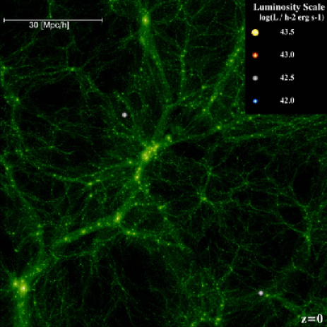
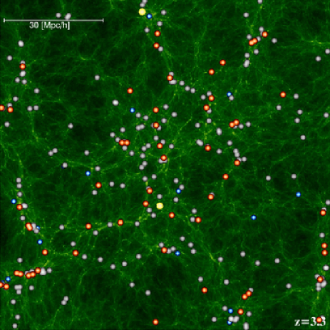
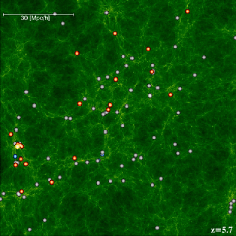
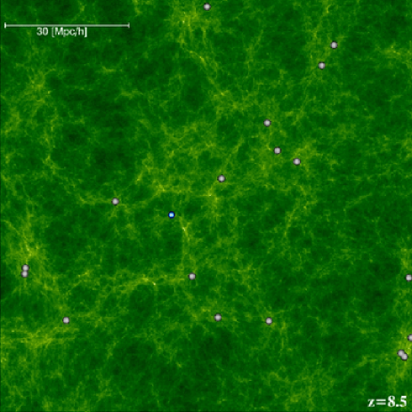
Figure 1: The spatial distribution of $\mathrm{Ly}\alpha$ emitting galaxies (coloured circles) in a slice from the Millennium simulation, with the dark matter distribution in green. The four panels are for redshifts in the range $0<z<8.5$, as indicated in each panel. The colour of the circles changes with the $\mathrm{Ly}\alpha$ luminosity of the galaxies, as shown in the key in the upper-right corner of the first panel. Only galaxies brighter than $\log(\mbox{$L_{\mathrm{Ly}\alpha}$}\mbox{$[\mathrm{erg}\ \mathrm{s}^{-1}\ \mathrm{h}^{-2}]$})=42.2$ are plotted. Each image covers a square region $100\times 100\mbox{$h^{-1}\mathrm{Mpc}$}^{2}$ across and having a depth of 10$h^{-1}\mathrm{Mpc}$, which is less than one thousandth the volume of the full simulation box.

A critical assumption of the Baugh et al. model is that stars formed in starbursts have a top-heavy initial mass function (IMF), where the IMF is given by $\rm{d}N/\rm{d}\ln(m)\propto m^{-x}$ and $x=0$. Stars formed quiescently in discs have a solar neighbourhood IMF, with the form proposed by Kennicut (1983): $x=0.4$ for $m<1M_{\odot}$ and $x=1.5$ for $m>1M_{\odot}$. Both IMFs cover the mass range $0.15M_{\odot}<m<125M_{\odot}$. Within the framework of $\Lambda$CDM, Baugh et al. argued that the top-heavy IMF is essential to match the counts and redshift distribution of galaxies detected through their sub-millimetre emission, whilst retaining the match to galaxy properties in the local Universe, such as the optical and far-IR luminosity functions and galaxy gas fractions and metallicities. Nagashima et al. (2005a, b) showed that such a top-heavy IMF also results in predictions for the metal abundances in the intra-cluster medium and in elliptical galaxies in much better agreement with observations. Lacey et al. (2008) showed that the same model predicts galaxy evolution in the IR in good agreement with observations from Spitzer, and also discussed independent observational evidence for a top-heavy IMF.

Reionization is assumed in our model to occur at $\mbox{$z_{\rm{reion}}$}=10$ (Kogut et al., 2003; Dunkley et al., 2008). The photoionization of the intergalactic medium (IGM) is assumed to suppress the collapse and cooling of gas in haloes with circular velocities $V_{c}<60\rm{km/s}$ at redshifts $z<\mbox{$z_{\rm{reion}}$}$ (Benson et al., 2002). Recent calculations (Hoeft et al., 2006; Okamoto, Gao & Theuns, 2008) imply that the above parameter values overstate the impact of photoionization on gas cooling, and suggest that photoionization only affects smaller haloes with $V_{c}\la 30{\rm km/s}$. Our model predictions, for the range of $\mathrm{Ly}\alpha$ luminosities we consider in this paper, are not significantly affected by adopting the lower $V_{c}$ cut. We neglect any attenuation of the $\mathrm{Ly}\alpha$ flux by propagation through the IGM. This effect would suppress the observed $\mathrm{Ly}\alpha$ flux mainly for $z\ga\mbox{$z_{\rm{reion}}$}$, so this should only affect our results for very high redshifts ($z\ga 10$).

The model used to predict the luminosities and equivalent widths of the $\mathrm{Ly}\alpha$ galaxies is identical to that described in Le Delliou et al. (2005, 2006). The $\mathrm{Ly}\alpha$ emission is computed by the following procedure: (i) The integrated stellar spectrum of the galaxy is calculated, based on its star formation history, including the effects of the distribution of stellar metallicities, and taking into account the IMFs adopted for different modes of star formation. (ii) The rate of production of Lyman continuum (Lyc) photons is computed by integrating over the stellar spectrum, and assuming that all of these ionizing photons are absorbed by neutral hydrogen within the galaxy. We calculate the fraction of $\mathrm{Ly}\alpha$ photons produced by these Lyc photons, assuming Case B recombination (Osterbrock, 1989).

(iii) The observed $\mathrm{Ly}\alpha$ flux depends on the fraction of $\mathrm{Ly}\alpha$ photons which escape from the galaxy ($f_{\mathrm{esc}}$), which is assumed to be constant and independent of galaxy properties.

Calculating the $\mathrm{Ly}\alpha$ escape fraction from first principles by following the radiative transfer of the $\mathrm{Ly}\alpha$ photons is very demanding computationally. A more complete calculation of the escape fraction would have into account the structure and kinematic properties of the intestellar medium (ISM) (Zheng & Miralda-Escudé, 2002; Ahn, 2004; Verhamme et al., 2006). In our model, we adopt the simplest possible approach, which is to fix the escape fraction, $f_{\mathrm{esc}}$, to be the same for each galaxy, without taking into account its dust properties. This results in a surprisingly good agreement between the predicted number counts and luminosity functions of emitters and the available observations at $3\la z\la 7$ (Le Delliou et al., 2005, 2006). Le Delliou et al. (2005) chose $f_{\mathrm{esc}}=0.02$ to match the number counts at $z\approx 3$ at a flux $f\approx 2\times 10^{-17}{\rm ergcm^{-2}s^{-1}}$. The same value is used in this work. This value for the $\mathrm{Ly}\alpha$ escape fraction seems very small, but is consistent with direct observational estimates for low redshift galaxies: Atek et al. (2008) derive escape fractions for a sample of nearby star-forming galaxies by combining measurements of Ly$\alpha$, H$\alpha$ and H$\beta$, and find that most have escape fractions of 3% or less. Le Delliou et al. (2006) also showed that if a standard solar neighbourhhod IMF is adopted for all modes of star formation, then a substantially larger escape fraction would be required to match the observed counts of $\mathrm{Ly}\alpha$ emitters, and even then the overall match would not be as quite good as it is when the top-heavy IMF is used in bursts.

Once we obtain the galaxy properties from the semi-analytical model, we plant these galaxies into a N-body simulation, in order to add information about their positions and velocities. The simulation used here is the Millennium Simulation (Springel et al., 2005). This simulation adopts concordance values for the parameters of a flat $\Lambda$CDM model, $\Omega_{\rm{m}}=0.25$ and $\Omega_{\rm{b}}=0.045$ for the densities of matter and baryons at $z=0$, $\mathrm{h}=0.73$ for the present-day value of the dimensionless Hubble constant, $\sigma_{8}=0.9$ for the rms linear mass fluctuations in a sphere of radius $8\mathrm{h}^{-1}$Mpc at $z=0$ and $n=1$ for the slope of the primordial fluctuation spectrum. The simulation follows $2160^{3}$ dark matter particles from $z=127$ to $z=0$ within a cubic region of comoving length $500\mathrm{h}^{-1}\mathrm{Mpc}$. The individual particle mass is $8.6\times 10^{8}\mathrm{h}^{-1}\mathrm{M_{\odot}}$, so the smallest dark halo which can be resolved has a mass of $2\times 10^{10}\mathrm{h}^{-1}\mathrm{M_{\odot}}$.

Dark matter haloes are identified using a Friends-Of-Friends (FOF) algorithm. To populate the simulation with galaxies from the semi-analytical model, we use the same approach as in Benson et al. (2000). First, the position and velocity of the centre of mass of each halo is recorded, along with the positions and velocities of a set of randomly selected dark matter particles from each halo. Second, the list of halo masses is fed into the semi-analytical model in order to produce a population of galaxies associated with each halo. Each galaxy is assigned a position and velocity within the halo. Since the semi-analytical model distinguishes between central and satellite galaxies, the central galaxy is placed at the centre of mass of the halo, and any satellite galaxy is placed on one of the randomly selected halo particles. Once galaxies have been generated, and positions and velocities have been assigned, it is a simple process to produce catalogues of galaxies with spatial information and any desired selection criteria.

The combination of the semi-analytical model with the N-body simulation is essential to study the detailed clustering of a desired galaxy population, although the clustering amplitude on large scales can also be estimated analytically (Le Delliou et al., 2006). An example of the output of the simulation is shown in the four images of Fig. 1 which show redshifts $z=0$, $z=3.3$, $z=5.7$ and $z=8.5$. The dark matter distribution (shown in green) becomes smoother as we go to higher redshifts, due to the gravitational growth of structures. As shown in Fig. 1, for this particular luminosity cut, the number density of $\mathrm{Ly}\alpha$ emitters varies at different redshifts. As we will show in the next section, these catalogues at high redshift are not complete at faint luminosities, so we have to restrict our predictions to brighter luminosities as we go to higher redshifts.

3 Luminosity Functions

The model presented by Le Delliou et al. (2005, 2006) differs in two main ways from the one presented in this paper: (i) there is a slight difference in the values of the cosmological parameters used, and (ii) the earlier work used a grid of halo masses together with an analytical halo mass function, rather than the set of haloes from an N-body simulation. In §3.1, we investigate the impact of the different choice of cosmological parameters on the luminosity function of $\mathrm{Ly}\alpha$ emitters, to see if the very good agreement with observational data obtained by Le Delliou et al. (2006) is retained on adopting the Millennium cosmology. In §3.2, we assess the completeness of our samples of $\mathrm{Ly}\alpha$ emitters due to the finite mass resolution of the Millennium simulation.

3.1 Comparison of model predictions with observed luminosity functions

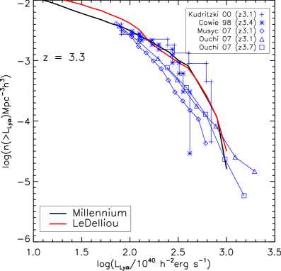
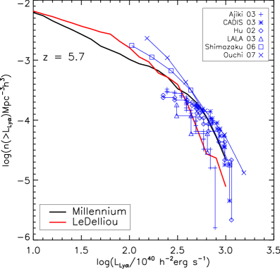
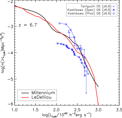
Figure 2: The cumulative luminosity functions of $\mathrm{Ly}\alpha$ emitters at redshifts $z=3.3$ (Top), $z=5.7$ (Center) and $z=6.7$ (Bottom). The blue points correspond to observational data (as indicated by the key with full references in the text). The black and red curves correspond, respectively, to the GALFORM predictions using the cosmological parameters of the Millennium Simulation and those adopted in Le Delliou et al.

In this section, we investigate the impact on the model predictions of the choice of cosmological parameters by re-running the model of Le Delliou et al. (2005, 2006), keeping the galaxy formation parameters the same but changing the cosmological parameters to match those used in the Millennium simulation. To recap, the original Le Delliou et al. (2006) model used $\Omega_{\rm{m}}=0.3$, $\Omega_{\Lambda}=0.7$, $\Omega_{\mathrm{b}}=0.04$ , $\sigma_{8}=0.93$ and $h=0.7$. In Fig. 2, we compare the cumulative luminosity functions obtained with GALFORM for the two sets of cosmological parameters with current observational data in the redshift range $3<z<7$. The observational data is taken from: Kudritzki et al. (2000) (crosses), Cowie & Hu (1998) (asterisks), Gawiser et al. (2007) (diamonds), Ouchi et al. (2007) (triangles and squares) in the $z=3.3$ panel; Ajiki et al. (2003) (pluses), Maier et al. (2003) (asterisks), Hu et al. (2004) (diamonds), Rhoads et al. (2003) (triangles), Shimasaku et al. (2006) (squares) and Ouchi et al. (2007) (crosses) in the $z=5.7$ panel; and Taniguchi et al. (2005) (crosses) and Kashikawa et al. (2006) (asterisks and diamonds) in the $z=6.7$ panel. At $z=3.3$, the two model curves agree very well, and are consistent with the observational data shown. At $z=5.72$, the two models do not match as well as in the previous case, but both are still consistent with the observational data. Finally, at $z=6.7$ the differences are small and both curves are consistent with observational data. The conclusion from Fig. 2 is that there is not a significant change in the model predictions on using these slightly different values of the cosmological parameters. Furthermore, the observational data is not yet sufficiently accurate to distinguish between the two models or to motivate the introduction of further modifications to improve the level of agreement, such as using a different $\mathrm{Ly}\alpha$ escape fraction.

3.2 The completeness of the Millennium galaxy catalogues

The Millennium simulation has a halo mass resolution limit of $1.72\times 10^{10}h^{-1}M_{\odot}$. In a standard GALFORM run, a grid of haloes which extends to lower mass haloes than the Millennium resolution is typically used, with $M_{\rm res}=5\times 10^{9}h^{-1}M_{\odot}$ at $z=0$. A fixed dynamic range in halo mass is adopted in these runs, but with the mass resolution shifting to smaller masses with increasing redshift: for our standard setup, we have $M_{\rm res}=7.8\times 10^{7}h^{-1}M_{\odot}$ and $1.4\times 10^{7}h^{-1}M_{\odot}$ at $z=3$ and $6$ respectively. Therefore, when putting GALFORM galaxies into the Millennium, our sample does not contain galaxies which formed in haloes with masses below the resolution limit of the Millennium. This introduces an incompleteness into our catalogues when compared to the original GALFORM prediction. The incompleteness of the galaxy catalogues is more severe for low luminosity galaxies because they tend to be hosted by low mass haloes, as will be shown in the next section. Hereafter, we will use N-body sample to refer to the GALFORM galaxies planted in the Millennium haloes, to distinguish them from the pure GALFORM catalogues generated using a grid of halos masses.

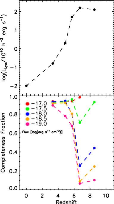
Figure 3: Completeness of the Millennium galaxy catalogues with respect to $\mathrm{Ly}\alpha$ luminosity or flux. (Top): The minimum luminosity down to which the catalogues are 85$\%$ complete. (Bottom): The completeness fraction as a function of redshift for a range of fluxes $-19<log(\mbox{$F_{\mathrm{Ly}\alpha}$}\mbox{$[\mathrm{erg}\ \mathrm{s}^{-1}\ \mathrm{cm}^{-2}]$})<-17$, as indicated by the key.

In order to quantify the incompleteness of the N-body sample as a function of luminosity, we define the completeness fraction as the ratio of the cumulative luminosity function for the N-body sample to that obtained for a pure GALFORM calculation, and look for the luminosity at which the completeness fraction deviates from unity. The panels of Fig. 3 give different views of the completeness of the N-body samples. The top panel shows the luminosity above which a catalogue can be considered as complete: we define the completeness limit as the luminosity at which the completeness fraction first drops to $0.85$. The figure clearly shows how the luminosity corresponding to this completeness limit becomes progressively brighter as we move to higher redshifts. For $z>9$ the N-body sample is incomplete at all luminosities plotted.

The bottom panel of Fig. 3 shows how the sample becomes more incomplete at any redshift as we consider fainter fluxes. A sample with galaxies brighter than $\log(\mbox{$F_{\mathrm{Ly}\alpha}$}\mbox{$[\mathrm{erg}\ \mathrm{s}^{-1}\ \mathrm{cm}^{-2}]$})=-19)$ is less than $70\%$ complete at all redshifts $z>5$, while a sample with galaxies brighter than $\log(\mbox{$F_{\mathrm{Ly}\alpha}$}\mbox{$[\mathrm{erg}\ \mathrm{s}^{-1}\ \mathrm{cm}^{-2}]$})=-17$ is always over $90\%$ complete for $z<9$. The completeness fraction monotonically decreases with increasing redshift until $z\sim 6$ for very faint fluxes. For $z>6$ the completeness rises again: the shape of the bright end of the luminosity function at this redshift is sensitive to the choice of the redshift of reionization.

In summary, the requirement that our samples be at least $80\%$ complete restricts the range of validity of the predictions from the Millennium simulation to redshifts below $9$, and fluxes brighter than $\log(\mbox{$F_{\mathrm{Ly}\alpha}$}\mbox{$[\mathrm{erg}\ \mathrm{s}^{-1}\ \mathrm{cm}^{-2}]$})>-17.5$.

4 Clustering Predictions

In this section we present clustering predictions using $\mathrm{Ly}\alpha$ emitters in the full Millennium volume. To study the clustering of galaxies we calculate the two-point correlation function, $\xi(r)$, of the galaxy distribution. In order to quantify the evolution of the clustering of galaxies, we measure the correlation function over the redshift interval $0<z<9$.

To calculate $\xi(r)$ in the simulaation, we use the standard estimator (e.g. Peebles 1980):

$$1+\xi(r)=\frac{\langle DD\rangle}{\frac{1}{2}N_{\rm gal}n\Delta V(r)},$$ (1)

where $\langle DD\rangle$ stands for the number of distinct data pairs with separations in the range $r$ to $r+\Delta r$, $n$ is the mean number density of galaxies, $N_{\rm gal}$ is the total number of galaxies in the simulation volume and $\Delta V(r)$ is the volume of a spherical shell of radius $r$ and thickness $\Delta r$. This estimator is applicable in the case of periodic boundary conditions. In the correlation function analysis, we consider two parameters which help us to understand the clustering behaviour of $\mathrm{Ly}\alpha$ galaxies: the correlation length, $r_{0}$, and the galaxy bias, $b$, both of which are discussed below.

4.1 Correlation Length evolution

A common way to characterize the clustering of galaxies is to fit a power-law to the correlation function:

$$\xi(r)=\left(\frac{r}{r_{0}}\right)^{-\gamma},$$ (2)

where $r_{0}$ is the correlation length and $\gamma=1.8$ gives a good fit to the slope of the observed correlation function over a restricted range of pair separations around $r_{0}$ at $z=0$ (e.g. Davis & Peebles (1983)). The correlation length can also be defined as the scale where $\xi=1$, and quantifies the amplitude of the correlation function when the slope $\gamma$ is fixed.

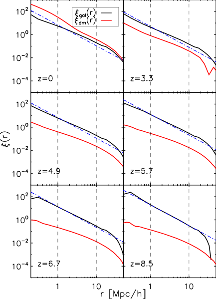
Figure 4: The correlation function predicted for $\mathrm{Ly}\alpha$ emitters (black solid curve) for a range of redshifts, as indicated in each panel. $\mathrm{Ly}\alpha$ emitters are included down to the completeness limit at each redshift shown in Fig 3. The solid red curve shows the correlation function of the dark matter at the same epochs. The blue dashed line shows the power law fit of Eq. (2), evaluated in the range $1<r[\mathrm{Mpc/h}]<10$, as delineated by the vertical dashed lines.

Fig. 4 shows the correlation function of $\mathrm{Ly}\alpha$ emitting galaxies, $\xi_{\mathrm{gal}}$ (solid black curves) of the full catalogues down to the completeness limits at each redshift, calculated using Eq. (1). The red curve shows $\xi_{\mathrm{dm}}$, the correlation function of the dark matter. At $z=0$, $\xi_{\mathrm{dm}}$ is larger than $\xi_{\mathrm{gal}}$, but for $z>0$ $\xi_{\mathrm{dm}}$ is increasingly below $\xi_{\mathrm{gal}}$. We will study in detail the comparison of the dark matter and $\mathrm{Ly}\alpha$ galaxy correlation functions in §4.2.

Another notable feature of Fig. 4 is that $\mbox{$\xi_{\mathrm{gal}}$}(r)$ differs considerably from a power law, particularly on scales greater than 10 $h^{-1}\mathrm{Mpc}$. When fitting Eq. (2) to the correlation functions plotted in Fig. 4, we use only the measurements in the range [1,10] $h^{-1}\mathrm{Mpc}$, where $\mbox{$\xi_{\mathrm{gal}}$}(r)$ behaves most like a power law. We fix the slope $\gamma=1.8$ for all $\mbox{$\xi_{\mathrm{gal}}$}(r)$ to allow a comparison between different redshifts, although we note that for $z<5$, the slope of $\mbox{$\xi_{\mathrm{gal}}$}(r)$ is closer to $\gamma=1.6$. By using the power law fit we can compare the clustering amplitudes of different galaxy samples. To determine the clustering evolution of $\mathrm{Ly}\alpha$ emitters, we split the catalogues of $\mathrm{Ly}\alpha$ emitters into luminosity bins. For each of these sub-samples, we calculate the correlation function and then we obtain $r_{0}$ by fitting Eq. (2) as described. Fig. 5 (top) shows the dependence of $r_{0}$ on luminosity for different redshifts in the range $0<z<9$. The errors are shown by the area enclosed by the thin solid lines for each set of points, and are calculated as the $90\%$ confidence interval of the $\chi^{2}$ fit of the correlation functions to Eq. (2) (ignoring any covariance between pair separation bins). The range of luminosities plotted is set by the completeness limit of the simulation described in the previous section. We also discard galaxy samples with fewer than 500 galaxies, as in such cases, the errors are extremely large and the correlation functions are poorly defined. The clustering in high redshift surveys of $\mathrm{Ly}\alpha$ emitters is sensitive to the flux limit that they are able to reach, as shown by Fig. 5.

The model predictions show modest evolution of $r_{0}$ with redshift for most of the luminosity range studied. Over this redshift interval, on the other hand, the correlation length of the dark matter changes dramatically, as shown by Fig. 4. Typically, at a given redshift, we find that $r_{0}$ shows little dependence on luminosity until a luminosity of $L_{\mathrm{Ly}\alpha}$$\sim 10^{42}\mbox{$[\mathrm{erg}\ \mathrm{s}^{-1}\ \mathrm{h}^{-2}]$}$ is reached, brightwards of which there is a strong increase in clustering strength with luminosity. This trend is even more pronounced at higher redshifts. Galaxies at $z=0$ are less clustered than galaxies in the range $3<z<7$, except at luminosities close to $L_{\mathrm{Ly}\alpha}$$\sim 10^{40}\mbox{$[\mathrm{erg}\ \mathrm{s}^{-1}\ \mathrm{h}^{-2}]$}$. At $z=8.5$, $r_{0}$ increases from $r_{0}\sim 5$ $h^{-1}\mathrm{Mpc}$ at $L_{\mathrm{Ly}\alpha}$$\sim 10^{42}\mbox{$[\mathrm{erg}\ \mathrm{s}^{-1}\ \mathrm{h}^{-2}]$}$ to $r_{0}\sim 12$ $h^{-1}\mathrm{Mpc}$ at $L_{\mathrm{Ly}\alpha}$$>10^{42.5}\mbox{$[\mathrm{erg}\ \mathrm{s}^{-1}\ \mathrm{h}^{-2}]$}$.

The growth of $r_{0}$ with limiting luminosity is related to the masses of the haloes which host $\mathrm{Ly}\alpha$ galaxies. As shown in the bottom panel of Fig. 5, there is not a simple relation between the median mass of the host halo and the luminosity of $\mathrm{Ly}\alpha$ emitters. For a given luminosity, $\mathrm{Ly}\alpha$ galaxies tend to be hosted by haloes of smaller masses as we go to higher redshifts. In addition, for redshifts $z>0$, there is a trend of more luminous $\mathrm{Ly}\alpha$ emitters being found in more massive haloes. The key to explaining the trends in clustering strength is to compare how the effective mass of the haloes which host $\mathrm{Ly}\alpha$ emitting galaxies is evolving compared to the typical or characteristic mass in the halo distribution ($M_{*}$) (Mo & White, 1996); if $\mathrm{Ly}\alpha$ emitters tend to be found in haloes more massive than $M_{*}$, then they will be more strongly clustered than the dark matter. This difference between the clustering amplitude of galaxies and mass is explored more in the next section. In a hierarchical model for the growth of structures, haloes more massive than $M_{*}$ are more clustered, and thus we expect a strong connection between the evolution of $r_{0}$ and the masses of the halos. Fig. 5 shows that the dependence of $r_{0}$ (and host halo mass) on luminosity becomes stronger at higher redshifts.

4.2 The bias factor of $\mathrm{Ly}\alpha$ emitters

The galaxy bias, $b$, quantifies the strength of the clustering of galaxies compared to the clustering of the dark matter. One way to calculate the bias is by taking the ratio of $\xi_{\mathrm{gal}}$ and $\xi_{\mathrm{dm}}$, $\mbox{$\xi_{\mathrm{gal}}$}=b^{2}\mbox{$\xi_{\mathrm{dm}}$}$. Both correlation functions are estimated using Eq. (1). Since the simulation contains ten billion dark matter particles, a direct pair-count calculation of $\xi_{\mathrm{dm}}$ would demand a prohibitively large amount of computer time, so we extract dilute samples of the dark matter particles, selecting randomly $\sim 10^{7}$ particles. In this way we only enlarge the pair-count errors on $\xi_{\mathrm{dm}}$ (which nevertheless are still much smaller than for $\xi_{\mathrm{gal}}$) but obtain the correct amplitude of correlation function itself.

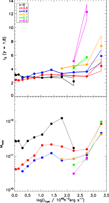
Figure 5: (Top): The evolution of the correlation length $r_{0}$ as a function of $\mathrm{Ly}\alpha$ luminosity for several redshifts in the range $0<z<9$, as indicated by the key. The thin solid coloured lines shows the errors on the correlation length. (Bottom): The evolution of the median mass of halos which host $\mathrm{Ly}\alpha$ emitting galaxies as a function of $\mathrm{Ly}\alpha$ luminosity, for the same range of redshifts as above.

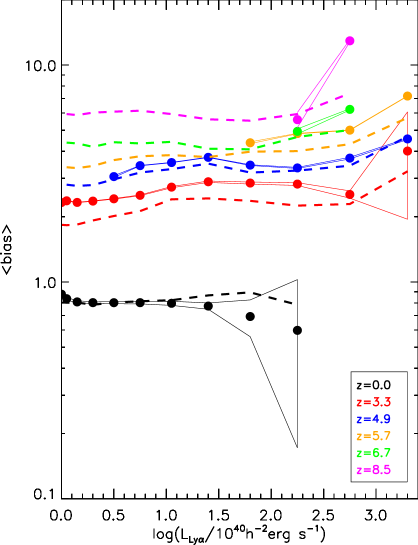
Figure 6: The galaxy bias as a function of $\mathrm{Ly}\alpha$ luminosity at different redshifts, as indicated by the key. The solid lines show the results from the simulation and the dashed lines show the analytical expression of SMT. The area enclosed by the thin solid lines shows the error on the bias estimation for each redshift.

To obtain the bias parameter of $\mathrm{Ly}\alpha$ emitters as a function of luminosity, we split the full catalogue of galaxies at each redshift into luminosity bins. For each of these bins we calculate $\xi_{\mathrm{gal}}$ and divide by $\xi_{\mathrm{dm}}$ to get the sqaure of the bias. Due to non-linearities, the ratio of $\xi_{\mathrm{gal}}$ and $\xi_{\mathrm{dm}}$ is not constant on all scales. As a reasonable estimation of the bias we chose the mean value over the range 6 $h^{-1}\mathrm{Mpc}$ $<r<$ 30 $h^{-1}\mathrm{Mpc}$. Over these scales the bias does seem to be constant and independent of scale. This range is quite similar to the one used by Gao, Springel & White (2005) to measure the bias parameter of dark matter haloes in the Millennium Simulation.

The bias parameter can also be calculated approximately using various analytical formalisms (Mo & White, 1996; Sheth, Mo & Tormen, 2001; Mandelbaum et al., 2005). These procedures relate the halo bias to $\sigma(m,z)$, the rms linear mass fluctuation within a sphere which on average contains mass $m$. The bias factor for galaxies of a given luminosity is then obtained by averaging the halo bias over the halos hosting these galaxies. Le Delliou et al. (2006) used the analytical expression of Sheth, Mo & Tormen (2001) (hereafter SMT) to calculate the bias parameter for the semi-analytical galaxies. This gives a reasonable approximation to the large-scale halo bias measured in N-body simulations (e.g (2008)).

Fig. 6 shows the bias parameter as a function of luminosity for redshifts in the range $0<z<9$, and compares the direct calculation using the N-body simulation (solid lines) with the analytical estimation (dashed lines). In order to calculate the uncertainty in our value of the bias, we assume an error on $\mbox{$\xi_{\mathrm{gal}}$}(r)$ of the form $\Delta\xi_{\mathrm{gal}}=2\sqrt{(1+\xi_{\mathrm{gal}})/DD}$ (Hewitt, 1982; Baugh et al., 1996), and assuming a negligible error in $\xi_{\mathrm{dm}}$ we get

$$\Delta b=\frac{1}{b\xi_{\mathrm{dm}}}\sqrt{\frac{1+b^{2}\xi_{\mathrm{dm}}}{DD}},$$ (3)

for the error in the bias estimation. This error is shown in Fig. 6 as the range defined by the thin solid lines surrounding the bias measurement shown by the points.

The first noticeable feature of Fig. 6 is the strong evolution of bias with increasing redshift: From $z=0$ to $z=8.5$ the bias factor increases from $b(z=0)\sim 0.8$ to $b(z=8.5)\sim 12$, which means that the clustering amplitude of $\mathrm{Ly}\alpha$ emitters at $z=8.5$ is over 140 times the clustering amplitude of the dark matter at this redshift. Another interesting prediction is the dependence of bias on $\mathrm{Ly}\alpha$ luminosity. For $z>3$ there seems to be a strong increase of the bias with luminosity for bins where $L_{\mathrm{Ly}\alpha}$ $>10^{42}\mbox{$[\mathrm{erg}\ \mathrm{s}^{-1}\ \mathrm{h}^{-2}]$}$. The agreement between the analytic calculation of the bias and the simulation result is reasonable over the range $0<z<5$, but becomes less impressive as higher biases are reached. A similar discrepancy was also noticed by Gao, Springel & White (2005), where they compared the halo bias extracted from the simulation with different analytic formulae (see also (2008)).

Another way to describe galaxy clustering is through the halo occupation distribution (HOD; Benson et al. (2000), Berlind et al. (2003), Cooray & Sheth (2002)). The HOD gives the mean number of galaxies which meet a particular observational selection as a function of halo mass. For flux-limited samples, the HOD can be broken down into the contribution from central galaxies and satellite galaxies. In a simple picture, the mean number of central galaxies is zero below some threshold halo mass, $M_{min}$, and unity for higher halo masses. With increasing halo mass, a second threshold is reached, $M_{crit}$, above which a halo can also host a satellite galaxy. The number of satellites is usually described by a power-law of slope $\beta$. In the simplest case, three parameters are needed to describe the HOD (Berlind et al., 2002; Hamana et al., 2004); more detailed models have been proposed to describe the transition from 0 to 1 galaxy (Berlind et al., 2003).

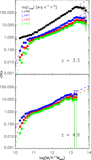
Figure 7: The HOD of $\mathrm{Ly}\alpha$ emitters at $z=3.3$ (top) and $z=4.9$ (bottom). Each set of points represents a model sample with a different luminosity limit, as given by the key in the upper panel. The dashed line in each panel correspond to a “best” fit using the Berlind et al. (2003) parametrization.

We can compute the HOD directly from our model. The results are shown in Fig. 7, where we plot the HOD at two different redshifts for different luminosity limits. For comparison, we plot the HOD parametrization of Berlind et al. (2003) against our model predictions. In general, this HOD does a reasonable job of describing the model output, and is certainly preferred over a simple three parameter model. However, for the $z=3.3$ case (top panel of Fig. 7), the shape of the model HOD for $\log(M/M_{\odot})>13$ is still more complicated than can be accommodated by the Berlind et al. parametrization, showing a flattening in the number of satellites as a function of increasing halo mass. There is less disagreement in the $z=4.9$ case (bottom panel), but our model HOD becomes very noisy for large halo masses.

5 Mock Catalogues

Table 1: Summary of survey properties and simulation results.

(1)	(2)	(3)	(4)	(5)	(6)	(7)	(8)	(9)	(10)	(11)
Survey	$z_{\mathrm{survey}}$	$z_{\mathrm{simulation}}$	$\Delta z$	Area $\mbox{$\mathrm{[arcmin]}$}^{2}$	$EW_{\mathrm{obs}}$[Å]	$F_{\mathrm{Ly}\alpha}$$[\mathrm{erg}\ \mathrm{s}^{-1}\ \mathrm{cm}^{-2}]$	$N_{\mathrm{obs}}$	$N^{\mathrm{median}}_{\rm{mock}}$	10-90%	$C_{v}$
MUSYC	3.1	3.06	0.04	961	80	$1.5\times 10^{-17}$	162	142	89-207	0.41
SXDS	3.1	3.06	0.06	3538	328	$1.1\times 10^{-17}$	356	316	256-379	0.19
	3.7	3.58	0.06	3474	282	$2.7\times 10^{-17}$	101	80	60-110	0.31
	5.7	5.72	0.10	3722	335	$7.4\times 10^{-18}$	401	329	255-407	0.23
ELVIS	8.8	8.54	0.10	$\sim 3160$	100	$3.7\times 10^{-18}$	–	20	14-29	0.37

Column (1) gives the name of the survey; (2) and (3) show the redshift of the observations and nearest output from the simulations, respectively; (4) shows the redshift width of the survey, based on the FWHM filter width; (5) shows the area covered by each survey; (6) and (7) show the equivalent width and $\mathrm{Ly}\alpha$ flux limits of the samples, respectively; (8) shows the number of galaxies detected in each survey; (9) and (10) show the median of the number of galaxies and the 10-90 percentile range found in the mock catalogues for each survey. Finally, column (11) gives the fractional variation of the number of galaxies, defined in Eq. (13).

In this section we make mock catalogues of $\mathrm{Ly}\alpha$ emitters for a selection of surveys. In the previous section, we used the full simulation box to make clustering predictions, exploiting the periodic boundary conditions of the computational volume. The simulation is so large that it can accommodate many volumes equivalent to those sampled by current $\mathrm{Ly}\alpha$ surveys, allowing us to examine the fluctuations in the number of emitters and their clustering. The characteristics of the surveys we replicate are listed in Table 1.

The procedure to build the mock catalogues is the following:

1. We extract a catalogue of galaxies from an output of the Millennium Simulation that matches (as closely as possible) the redshift of a given survey. The simulation output contains 64 snapshots spaced roughly logarithmically in the redshift range $[127,0]$.

2. We choose one of the axes (say, the z-axis) as the line-of-sight, and we convert it to redshift space, to match what is observed in real surveys. To do this we replace $r_{z}$ (the comoving space coordinate) with

   $$s_{z}=r_{z}+\frac{v_{z}}{a\rm{H(z)}}\quad[\mbox{$h^{-1}\mathrm{Mpc}$}],$$ (4)

   where $v_{z}$ is the peculiar velocity along the z-axis, $a=1/(1+z)$ and H($z$) is the Hubble parameter at redshift $z$.

3. We then apply the flux limit of the particular survey, to mimic the selection of galaxies. Table 1 shows the flux limits of the surveys considered.

4. Then we extract many mock catalogues using the same geometry as the real survey. We extract slices of a particular depth $\Delta z$ (different for each survey), and within each slice we extract as many mock catalogues as possible using the same angular geometry as the real sample. $\Delta z$ is determined using the transmission curves of the narrow-band filters used in each survey. To derive the angular sizes we use:

   $$D_{t}(\theta,z)=d_{c}(z)\Delta\theta,$$ (5)

   $$d_{c}(z)=\frac{c}{H_{0}}\int_{0}^{z}\frac{{\rm d}z^{\prime}}{\sqrt{\Omega_{m}(1+z^{\prime})^{3}+\Omega_{\Lambda}}},$$ (6)

   where $D_{t}$ is the transverse comoving size in $h^{-1}$Mpc, $d_{c}$ is the comoving radial distance, $c$ and $H_{0}$ are the speed of light and the Hubble constant respectively, $\Omega_{\rm m}$ and $\Omega_{\Lambda}$ are the density parameters of matter and the cosmological constant respectively. Eq. (5) is valid for $\Delta\theta\ll 1[\rm{radians}]$, which is the case for the surveys we analyse in this work. We assume a flat cosmology.

5. From the line-of-sight axis we invert Eq. (6) to obtain the redshift distribution of $\mathrm{Ly}\alpha$ galaxies within each mock catalogue, converting galaxy position to redshift. This information is then used to take into account the shape of the filter transmission curve for each survey, which controls the minimum flux and equivalent width as a function of redshift. The value given in Table 1 corresponds to the minimum flux and $EW_{\mathrm{obs}}$ at the peak of the filter transmission curve. For redshifts at which the transmission is smaller (the tails of the curve) the minimum flux and $EW_{\mathrm{obs}}$ required for a $\mathrm{Ly}\alpha$ emitter to be included are proportionally bigger.

6. Finally, we allow for incompleteness in the detection of $\mathrm{Ly}\alpha$ emitters at a given flux due to noise in the observed images (where this information is available). To do this, we randomly select a fraction of galaxies in a given $\mathrm{Ly}\alpha$ flux bin to match the completeness fraction reported for the survey at that flux.

Real surveys of $\mathrm{Ly}\alpha$ emitters usually lack detailed information about the position of galaxies along the line-of-sight. Hence, instead of measuring the spatial correlation function defined in Eq. (1), it is only possible to estimate the angular correlation function, $w(\theta)$, which is the projection on the sky of $\xi(r)$.

We estimate $w(\theta)$ from mock catalogues using the following procedure, which closely matches that used in real surveys. To compute the angular correlation function we use the estimator (Landy & Szalay, 1993):

$$w_{LS}(\theta)=\frac{\langle DD(\theta)\rangle-2\langle DR(\theta)\rangle+\langle RR(\theta)\rangle}{\langle RR(\theta)\rangle},$$ (7)

where $\langle DR\rangle$ stands for data-random pairs, $\langle RR\rangle$ indicates the number of random-random pairs and all of the pair counts have been appropriately normalized. In the case of a finite volume survey, this estimator is more robust than the one defined in Eq. (1) because it is less sensitive to errors in the mean density of galaxies, such as could arise from boundary effects. In practice, the measured angular correlation function can be approximated by a power law:

$$w(\theta)=A_{w}\left(\frac{\theta}{1^{\circ}}\right)^{-\delta},$$ (8)

where $A_{w}$ is the dimensionless amplitude of the correlation function, and $\delta$ is related to slope of the spatial correlation function, $\gamma$, from Eq. (2) by $\delta=\gamma-1$. A relation between $r_{0}$ and $A_{w}$ can be obtained using a generalization of Limber’s equation (Simon, 2007).

Surveys of $\mathrm{Ly}\alpha$ emitters typically cover relatively small areas of sky and can display significant clustering even on the scale of the survey. As a result, the mean galaxy number density within the survey area will typically differ from the cosmic mean value. If the number of galaxies within the survey is used to estimate the mean density, used in Eq. (7), rather than the unknown true underlying density, this leads to a bias in the estimated correlation function. This effect is known as the integral constraint (IC) bias. Landy & Szalay (1993) show that when their estimator is used, the expected value of the estimated correlation function $w_{LS}(\theta)$ is related to the true correlation function $w(\theta)$ by

$$\langle w_{LS}(\theta)\rangle=\frac{w(\theta)-w_{\Omega}}{1+w_{\Omega}},$$ (9)

where the integral constraint term $w_{\Omega}$ is defined as

$$w_{\Omega}\equiv\frac{1}{\Omega^{2}}\int d\Omega_{1}d\Omega_{2}w(\theta_{12}),$$ (10)

integrating over the survey area, and is equal to the fractional variance in number density over that area.

When the clustering is weak Eq. (9) simplifies to $\langle w_{LS}(\theta)\rangle\simeq w(\theta)-w_{\Omega}$. This motivates the additive IC correction which is customarily used in practice:

$$w_{corr}(\theta)=w_{LS}(\theta)+w_{\Omega}.$$ (11)

We use this to correct the angular correlation functions from our mock catalogues. In order to estimate the term $w_{\Omega}$, we approximate the true correlation function as a power law, as in Eq. (8), and use

$$w_{\Omega}\simeq A_{w}\frac{\sum_{i}\langle RR_{i}\rangle\theta_{i}^{-\delta}}{\sum\langle RR_{i}\rangle},$$ (12)

(, 2000), where $\langle RR\rangle$ are the same random pairs as used in the estimate of $w_{LS}(\theta)$.

To quantify the sample variance expected for a particular survey, we use the mock catalogues to calculate a coefficient of variance ($C_{v}$), which is a measure of the fractional variation in the number of galaxies found in the mocks

$$C_{v}=\frac{N_{90}-N_{10}}{2N_{\rm{med}}},$$ (13)

where $N_{10}$ and $N_{90}$ are the 10 and 90 percentiles of the distribution of the number of galaxies in the mocks, respectively, and $N_{\rm{med}}$ is the median. The value of $C_{v}$ allows us to compare the sampling variance between different surveys in a quantitative way.

To analyse the clustering in the mock catalogues, we measured the angular correlation function of each mock catalogue using the procedure explained above. Then we fit Eq. (8) to each of the mock $w(\theta)$ and we choose the median value of $A_{w}$ as the representative power law fit. We fix the slope of $w(\theta)$ to $\delta=0.8$ for all surveys, except for ELVIS, where we found that a steeper slope, $\delta=1.2$, agreed much better with the simulated data. To express the variation in the correlation function amplitude found in the mocks, we calculate the 10 and 90 percentiles of the distribution of $A_{w}$ for each set of mock surveys. We also calculate $w(\theta)$ using the full transverse extent of the simulation, with the same selection of galaxies as for the real survey. This estimate of $w(\theta)$, which we call the Model $w(\theta)$, represents an ideal measurement of the correlation function without boundary effects (so there is no need for the integral constraint correction).

The surveys we mimic are the following: the MUSYC Survey (Gronwall et al., 2007; Gawiser et al., 2007), which is a large sample of $\mathrm{Ly}\alpha$ emitting galaxies at $z=3.1$; the SXDS Survey (Ouchi et al., 2005, 2007), which covers three redshifts: $z=3.1$, $z=3.7$ and $z=5.7$, and finally, we make predictions for the forthcoming ELVIS survey (Nilsson et al., 2007a, b), which is designed to find $\mathrm{Ly}\alpha$ emitting galaxies at $z=8.8$. We now describe the properties of the mock catalogues for each of these surveys in turn.

5.1 The MUSYC Survey

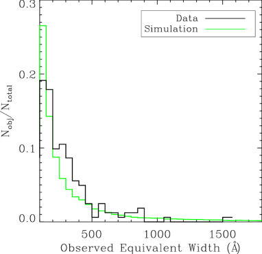
Figure 8: The observed $EW_{obs}$ distribution of the MUSYC survey at $z=3.1$ (solid black line) and the simulation (solid green line).

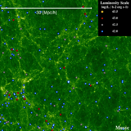
Figure 9: An image of a mock catalogue of the MUSYC Survey of $\mathrm{Ly}\alpha$ emitters at $z=3.1$. The colour format and legend are the same as used in Fig. 1. The angular size of the image is $31\arcmin\times 31\arcmin$.

The Multi-wavelength Survey by Yale-Chile (MUSYC) (Quadri et al., 2007; Gawiser et al., 2006, 2007; Gronwall et al., 2007) is composed of four fields covering a total solid angle of one square degree, each one imaged from the ground in the optical and near-infrared. Here we use data from a single MUSYC field consisting of narrow-band observations of $\mathrm{Ly}\alpha$ emitters made with the CTIO 4-m telescope in the Extended Chandra Deep Field South (ECDFS) (Gronwall et al., 2007). The MUSYC field, centred on redshift $z=3.1$, contains 162 $\mathrm{Ly}\alpha$ emitters in a redshift range of $\Delta z\sim 0.04$ over a rectangular area of $31\arcmin\times 31\arcmin$ with flux and $EW_{\mathrm{obs}}$ limits described in Table 1.

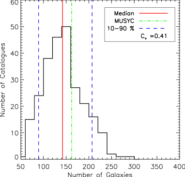
Figure 10: Histogram of the number of $\mathrm{Ly}\alpha$ emitters found in the mock MUSYC catalogues. The red line shows the median, the dashed blue lines show the 10-90 percentile range, and the green line shows the number of galaxies detected in the real survey.

To test how well the model reproduces the $\mathrm{Ly}\alpha$ emitters seen in the MUSYC survey, we first compare the predicted (green) and measured (black) distributions of $\mathrm{Ly}\alpha$ equivalent widths in Fig. 8. Here the predicted distribution comes from the full simulation volume. Overall, the simulation shows remarkably good agreement with the real data, with a slight underestimation in the range $200<\mbox{$EW_{\mathrm{obs}}$}[$Å$]<400$. For $\mbox{$EW_{\mathrm{obs}}$}[$Å$]>400$ both distributions seem to agree well, although the number of detected $\mathrm{Ly}\alpha$ emitters in the tail of the distribution is small.

For the MUSYC survey we built $252$ mock catalogues from the Millennium simulation volume using the procedure outlined above. Fig. 9 shows an example of one of these mock catalogues. Many of the $\mathrm{Ly}\alpha$ emitters are found in high dark matter density regions, and thus they are biased tracers of the dark matter. Fig. 10 shows the distribution of the number of galaxies in the ensemble of mocks. The green line shows the number detected in the real survey (162), which falls within the 10-90 percentile range of the mock distribution and is close to the median (142). The 10-90 percentile range spans an interval of $89<N_{\rm{gal}}<207$, indicating a large cosmic variance for this survey configuration, with $C_{v}=0.41$.

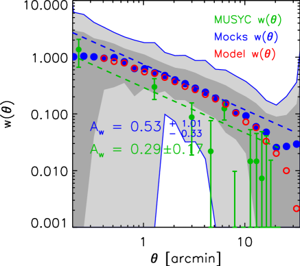
Figure 11: Angular clustering for the MUSYC Survey. Green circles show $w(\theta)$ calculated from the observed catalogue (Gawiser et al., 2007). The blue circles show the median $w(\theta)$ from all mock catalogues, corrected for the integral constraint effect. The dark and light grey shaded regions respectively show the 68% and 95% ranges of the distribution of $w(\theta)$ measured in the mock catalogues. The red open circles show the Model correlation function, obtained using the width of the entire simulation box (and the same EW, flux and redshift limits). The dashed lines show the power-law fit to the observed $w(\theta)$ (green) and the median fit to $w(\theta)$ from the mock catalogues (blue). The amplitudes $A_{w}$ of these fits are also given in the figure.

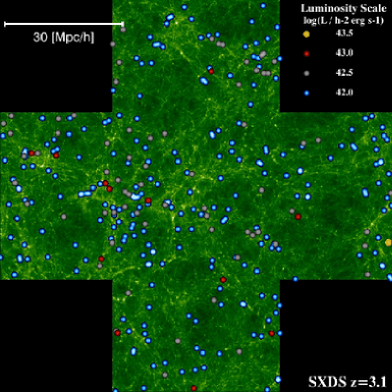
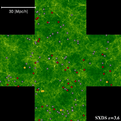
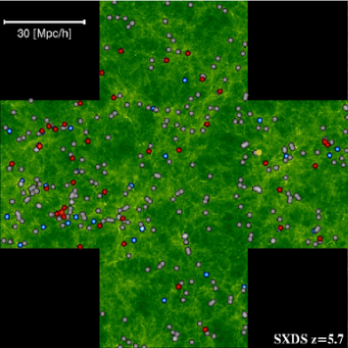
Figure 12: Mock catalogues of the SXDS survey for redshifts $3.1$ (top), $3.6$ (centre) and $5.7$ (bottom). The colour scheme and legend are the same as used previously. The angular size of the image is $1.4^{\circ}\times 1.4^{\circ}$.

The next step is to compare the clustering in the simulations with the real data. Fig. 11 plots the correlation functions from the mock catalogues alongside that measured in the real survey (Gawiser et al., 2007). There is reasonable agreement between the mock catalogue results and the observed data . The median $w(\theta)$ from the mocks is slightly higher than the observed values, but the observed $w(\theta)$ is within the range containing 95% of the mock $w(\theta)$ values (i.e. between the 2.5% and 97.5% percentiles, shown by the light grey shaded region). We quantified this difference by fitting the power law of Eq. (8) to both real and mock data. The power-law fits were made over the angular range 1-10 arcmins. We find the value of $A_{w}$ (Eq. 8) for each of the mock catalogue correlation functions by $\chi^{2}$-fitting (using the same expression as in §4.2 for the error on each model datapoint) and then we plot the power law corresponding to the median value of $A_{w}$. We find $A_{w}=0.53^{+1.01}_{-0.33}$ for the mocks, where the central value is the median, and the range between the error bars contains 95% of the values from the mocks. For the real data, we find the best-fit $A_{w}$ and the 95% confidence interval around it by $\chi^{2}$-fitting, using the error bars on the individual datapoints reported by Gawiser et al.. This gives $A_{w}=0.29\pm 0.17$ for the real data. We again see that the observed value is within the 95% range of the mocks, and is thus statistically consistent with the model prediction. We also see that the 95% confidence error bar on the observed $A_{w}$ is much smaller than the error bar we find from our mocks. This latter discrepancy arises from the small errors quoted on $w(\theta)$ by Gawiser et al. (2007), which are based on modified Poisson pair count errors, but neglect variations between different sample volumes (i.e. cosmic variance). On the contrary, using our mocks, we are able to take cosmic variance fully into account. This underlines the importance of including the cosmic variance in the error bars on observational data, to avoid rejecting models by mistake.

The red open circles in Fig. 11 show the correlation function obtained using the full angular size attainable with the Millennium simulation but keeping the same flux, EW and redshift limits as in the MUSYC survey (averaging 7 different slices), and so this measurement has a smaller sample variance. The area used here is $\sim 120$ times bigger than the MUSYC area, so IC effects are negligible on the scales studied here. We refer to this as the Model prediction for $w(\theta)$.

The median of the mock correlation functions (including the IC correction, blue circles) is seen to agree reasonably well with the Model correlation function (red open circles) for $\theta<20\mbox{$\mathrm{[arcmin]}$}$. This shows that for this survey it is possible to obtain an observational estimate of the correlation function which is unbiased over a range of scales, by applying the integral constraint correction. However, on large scales the median $w(\theta)$ of the mocks (with IC correction included) lies above the Model $w(\theta)$, which shows that the IC correction is not perfect, even on average. Presumably this failure is due (at least in part) to the fact that the IC correction procedure assumes that $w(\theta)$is a power law, while the true $w(\theta)$ departs from a power law on large scales. It is also important to note that these statements only apply to the median $w(\theta)$ derived from the mock samples - the individual mocks show a large scatter around the true $w(\theta)$ (as shown by the grey shading), and the IC correction does not remove this. This scatter rapidly increases at both small and large angular scales, so the best constraints on $w(\theta)$ from this survey are for intermediate scales, $1\la\theta\la 5\mbox{$\mathrm{[arcmin]}$}$.

5.2 The SXDS Surveys

The Subaru/XMM-Newton Deep Survey (SXDS) (Ouchi et al., 2005, 2007; Kashikawa et al., 2006) is a multi-wavelength survey covering $\sim 1.3$ square degrees of the sky. The survey is a combination of deep, wide area imaging in the X-ray with XMM-Newton and in the optical with the Subaru Suprime-Cam. Here we are interested in the narrow-band observations at three different redshifts: $3.1,3.6$ and $5.7$ (Ouchi et al., 2007).

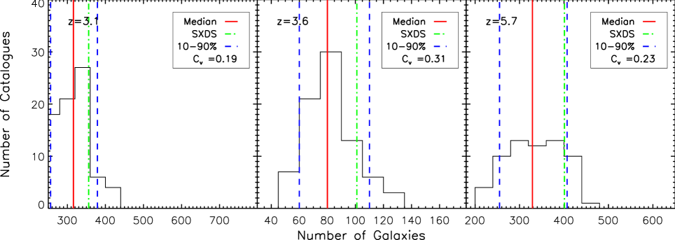
Figure 13: The distribution of the number of galaxies in mock SXDS catalogues, for $z=3.1$ (left), $z=3.6$ (centre) and $z=5.7$ (right). The red line shows the median of the number of galaxies inside the mock catalogues, the blue lines show the 10-90 percentiles of the distribution, and the green line shows the number observed in the SXDS.

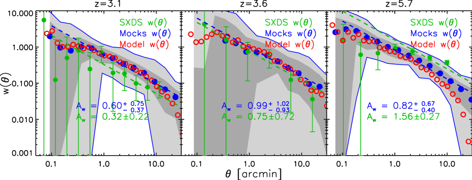
Figure 14: Angular correlation functions for the mock SXDS catalogues at $z=3.1$ (Left), $z=3.6$ (Center) and $z=5.7$ (Right). The blue circles show the median $w(\theta)$ from the mock catalogues (after applying the IC correction). The dark and light grey shaded regions respectively show the 68% and 95% ranges of the distribution of $w(\theta)$ measured in the mock catalogues. The red open circles are the Model $w(\theta)$ calculated using the full simulation width, averaged over many slices. The green circles show the observational data from Ouchi et al. The dashed lines show the power-law fit to the observed $w(\theta)$ (green) and the median fit to $w(\theta)$ from the mock catalogues (blue). The amplitudes $A_{w}$ of these fits are also given in the figure.

We build mock SXDS catalogues following the same procedure as outlined above. Fig. 12 shows examples of our mock catalogues for each redshift. As in the previous case, we see that $\mathrm{Ly}\alpha$ emitters on average trace the higher density regions of the dark matter distribution. The real surveys have a well defined angular size. However, the area sampled is slightly different at each redshift. In order to keep the cross-like shape in our mock catalogues and be consistent with the exact area surveyed, we scaled the cross-like shape to cover the same angular area as the real survey at each redshift.

Fig. 13 shows the distribution of the number of galaxies in the mock catalogues for the three redshifts surveyed. The median number of galaxies in the mocks at $z=3.1$ is 316, which is remarkably similar to the observed number, 356. The 10-90 percentile range of the mocks covers 256–379 galaxies. The coefficient of variation is $C_{v}=0.19$, less than half the value found for the MUSYC mock catalogues, $C_{v}=0.41$. This reduction is due mainly to the larger area sampled by the SXDS survey. In the second slice ($z=3.6$), the redshift is only slightly higher than in the previous case, but the number of galaxies is much lower. Looking at the top panel of Fig. 2 we see that the observed LFs are basically the same for these two redshifts. The difference between the two samples is explained mostly by the different $\mathrm{Ly}\alpha$ flux limits ($1.2\times 10^{-17}\mbox{$[\mathrm{erg}\ \mathrm{s}^{-1}\ \mathrm{cm}^{-2}]$}$ for $z=3.1$ and $2.6\times 10^{-17}\mbox{$[\mathrm{erg}\ \mathrm{s}^{-1}\ \mathrm{cm}^{-2}]$}$ for $z=3.6$). For the $z=3.6$ mocks, we find a median number of 80 and 10-90% range 60–110, in reasonable agreement with the observed number of galaxies, 101. The fractional variation in the number of galaxies, quantified by $C_{v}=0.31$, is larger than in the previous case, due to the smaller number of galaxies. The $z=5.7$ case is similar to the lower redshifts. The median number in the mocks is 329, with 10-90% range 255–407, again consistent with the observed number, 401. The coefficient of variation for this survey is $C_{v}=0.23$, so the sampling variance is intermediate between that for the $z=3.1$ and $z=3.6$ surveys.

The angular correlation functions of the mock catalogues are compared with the real data in Fig. 14. The observational data shown are preliminary angular correlation function measurements in the three SXDS fields, with errorbars based on bootstrap resampling (M. Ouchi, private communication). As in our comparison with the MUSYC survey, we plot the median correlation function measured from the mocks, after applying the IC correction, as a representative $w(\theta)$ . As before, we also perform a $\chi^{2}$ fit of a power law to the $w(\theta)$ measured in each mock, and to the observed values, to determine the amplitude $A_{w}$. The fit is performed over the range $1<\theta<10\mbox{$\mathrm{[arcmin]}$}$ as before.

The left panel of Fig. 14 shows the correlation functions at $z=3.1$. According to both the error bars on the observational data, and the scatter in $w(\theta)$ in the mocks (shown by the grey shading), this survey provides useful constraints on the clustering for $1\la\theta\la 10\mbox{$\mathrm{[arcmin]}$}$, but not for smaller or larger angles, where the scatter becomes very large. The fitted amplitude $A_{w}$ for the observed correlation function is $A_{w}=(0.32\pm 0.22)$ (95% confidence, using the error bars reported by Ouchi et al.), somewhat below the median value found in the mocks, $A_{w}=0.60$, but within the 95% range for the mocks ($A_{w}=0.23-1.35$). Based on the mocks, the model correlation function is consistent with the SXDS data at this redshift.

Comparing these results with those we found for the MUSYC survey (which has a very similar redshift and flux limit to SXDS at $z=3.1$), we see that the results seem very consistent. The MUSYC survey has a larger sample variance than SXDS, but the measured clustering amplitude is very similar in the two surveys.

The middle panel of Fig. 14 shows the correlation function for the $z=3.6$ survey. In this case, the error bars on the observational data and the scatter in the mocks are both larger, due to the lower surface density of galaxies in this sample. For the observed correlation amplitude, we obtain $A_{w}=0.75\pm 0.72$, while for the mocks we find a median $A_{w}=0.99$, with 95% range 0.06–2.01, entirely consistent with the observational data.

The right panel of Fig. 14 shows the correlation function predictions for $z=5.7$. According to the spread of mock catalogue results, the $w(\theta)$ measured here is the most accurate of the three surveys, due to the large number of galaxies. For the mocks, we find a median correlation amplitude $A_{w}=0.82$, with 95% range 0.42–1.49. For the observations, we find $A_{w}=1.56\pm 0.27$, if we assume a slope $\delta=0.8$. The average correlation function in the mocks agrees well with this slope over the range fitted, but the observational data for $w(\theta)$ at this redshift prefer a flatter slope. The model is however still marginally consistent with the observational data at 95% confidence. Similarly flat shapes were also found in some previous surveys (Shimazaku et al., 2004; Hayashino et al., 2004) in the same field, but at redshifts $3.1$ and $4.9$ respectively. However, these surveys are much smaller in terms of area surveyed and number of galaxies (this is particularly so in Shimazaku et al. (2004)). This behaviour in $w(\theta)$ might be produced by the high density regions associated with protoclusters in the SXDS fields (M. Ouchi, private communication), but still this behaviour of $w(\theta)$ must be confirmed to prove that it is a real feature of the correlation function.

5.3 ELVIS Survey

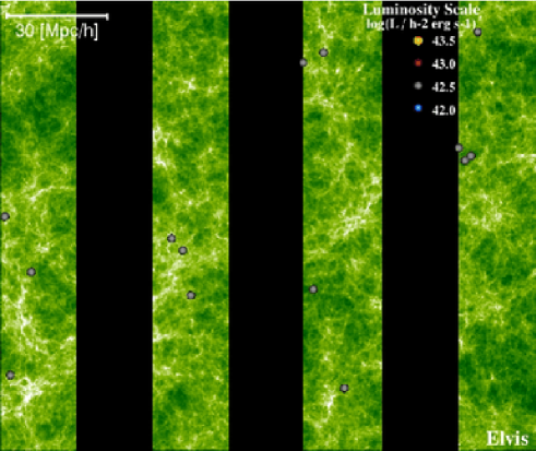
Figure 15: An example of a mock catalogue for the ELVIS Survey. The image shows the observed field of view (four strips). The legend and colour format are the same as in Figs.9 and 12.

One of the main goals of the public surveys planned for the Visible and Infrared Survey Telescope for Astronomy (VISTA) is to find a significant sample of very high redshift $(z\sim 8.8)$ $\mathrm{Ly}\alpha$ emitters. This program is called the Emission-Line galaxies with VISTA survey (ELVIS) (Nilsson et al., 2007a, b). The plan for ELVIS is to image four strips of $11.6\arcmin\times 68.27\arcmin$, covering a total area of 0.878$\mathrm{deg}^{2}$, as shown in Fig. 15. This configuration is dictated by the layout of the VISTA IR camera array. The only current detections of $\mathrm{Ly}\alpha$ emitters at $z>8$ are those of Stark et al. (2007), which have not yet been independently confirmed. $\mathrm{Ly}\alpha$ emitting galaxies at such redshifts will provide us with valuable insights into the reionization epoch of the Universe, as well as galaxy formation and evolution.

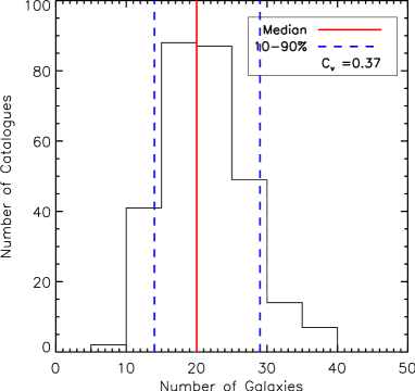
Figure 16: Histogram of the number of galaxies in mock catalogues expected for the ELVIS Survey. The red line shows the median of the distribution, and the blue dashed lines the 10-90 percentiles of the distribution.

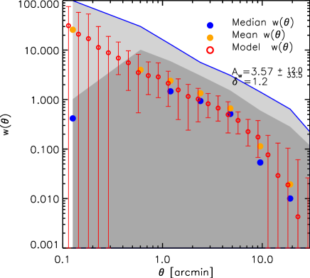
Figure 17: Angular Correlation Functions in the mock catalogues of the ELVIS Survey. The blue circles shows the median $w(\theta)$ from the mock catalogues, while the orange circles shows the mean. The dark and light grey shaded regions respectively show the 68% and 95% ranges of the distribution of $w(\theta)$ in the mocks. The red open circles show the Model $w(\theta)$  obtained using the full width of the simulation box. The amplitude and slope of the median power-law fit to the mocks are also given.

For our mock ELVIS catalogues, we select galaxies with a minimum flux of $\mbox{$F_{\mathrm{Ly}\alpha}$}=3.7\times 10^{-18}\mbox{$[\mathrm{erg}\ \mathrm{s}^{-1}\ \mathrm{cm}^{-2}]$}$ and $\mbox{$EW_{\mathrm{obs}}$}>100$ Å, as listed in Table 1. (The $EW_{\mathrm{obs}}$ limit is just a rough estimate, although our predictions should not be sensitive to the exact value chosen.) Fig. 15 shows the expected spatial distribution of $z=8.5$ galaxies in one of the ELVIS mock catalogues. Each mock catalogue has four strips, matching the configuration planned for the real survey. The median number of galaxies within the mock catalogues is 20, with a 10-90 percentile spread of 14 to 29 galaxies, as shown in Fig. 16. The fractional variation in number between different mocks is $C_{v}=0.37$, which is quite large, but no worse than for the MUSYC survey at $z=3.1$, even though that survey has 10 times as many galaxies.

The angular correlation functions of the mock ELVIS catalogues were calculated in the same way as before (including the integral constraint correction). Fig. 17 shows the median of the $w(\theta)$ values measured from each mock catalogue (blue circles), and also the mean (orange circles). In this case, the distribution of $w(\theta)$ values within each angle bin is very skewed, due to the small number of galaxies in the mock catalogues, and so the mean and median can differ significantly. The dark and light grey shaded regions show the ranges containing 68% and 95% of the $w(\theta)$ values from the mocks, from which it can be seen that the cosmic variance for this survey is very large. We also show the Model $w(\theta)$ (red circles), which provides our best estimate of the true correlation function based on the Millennium simulation, and was calculated by averaging over 10 slices of the simulation, using the full width of the simulation box. Even here, the error bars on $w(\theta)$ are quite large, due to the very low number density of galaxies predicted. We see that the mean and median $w(\theta)$ in the mocks lie close to the Model values for $2\mbox{$\mathrm{[arcmin]}$}<\theta<20\mbox{$\mathrm{[arcmin]}$}$, so in this sense they provide an unbiased estimate.

The most noticeable feature of Fig. 17 is the large area covered by both the 68% and 95% ranges of the distribution of $w(\theta)$ in the mocks, which extend down to $w(\theta)=0$. This indicates that the ELVIS survey will only be able to put a weak upper limit on the clustering amplitude of $z\sim 8.8$ $\mathrm{Ly}\alpha$ emitters, if our model is correct. As before, we can quantify this by fitting a power law to $w(\theta)$ in our mocks. We notice that the Model $w(\theta)$ for this sample has a significantly steeper slope, $\delta=1.2$, than the canonical value $\delta=0.8$, and so we do our fits to the mocks using $\delta=1.2$. We find a median amplitude in the mocks $A_{w}=3.57^{+12.0}_{-33.5}$, where the error bars give the 95% range.

6 Summary and conclusions

We have combined a semi-analytical model of galaxy formation with a high resolution, large volume N-body simulation to make predictions for the spatial distribution of $\mathrm{Ly}\alpha$ emitters in a $\Lambda$CDM universe.

Our model for $\mathrm{Ly}\alpha$ emitters is appealingly simple. Using the star formation history predicted for each galaxy from the semi-analytical model to compute the production of Lyman continuum photons, we find that on adopting a constant escape fraction of $\mathrm{Ly}\alpha$ photons the observed number of $\mathrm{Ly}\alpha$ emitters can be reproduced amazingly well over a range of redshifts (Le Delliou et al., 2006). Our modelling of $\mathrm{Ly}\alpha$ emission may appear overly simplistic on first comparison to other calculations in the literature. For example, Nagamine et al. (2008) predicted the clustering of $\mathrm{Ly}\alpha$ emitters in a gas-dynamic simulation, modelling the $\mathrm{Ly}\alpha$ emission through a $\mathrm{Ly}\alpha$ escape fraction or a duty cycle scenario. However, the fraction of active emitters in the duty cycle scenario needs to be tuned at each redshift, for which there is no physical justification. Since our predictions for $\mathrm{Ly}\alpha$ emission are derived from a full model of galaxy formation, it is straightforward to extract other properties of the emitters, such as their stellar mass or the mass of their host dark matter halo (Le Delliou et al. 2006). In this paper we have extended this work to include explicit predictions for the spatial and angular clustering of $\mathrm{Ly}\alpha$ emitters.

We have studied how the clustering strength of $\mathrm{Ly}\alpha$ emitters depends upon their luminosity as a function of redshift. Generally, we find that $\mathrm{Ly}\alpha$ emitters show a weak dependence of clustering strength on luminosity, until the brightest luminosities we consider are reached. At the present day, $\mathrm{Ly}\alpha$ emitters display weaker clustering than the dark matter. This changes dramatically at higher redshifts ($z>3$), with currently observable $\mathrm{Ly}\alpha$ emitters predicted to be much more strongly clustered than the dark matter, with the size of the bias increasing with redshift. We compared the simulation results with analytical estimates of the bias. Whilst the analytical results show the same trends as the simulation results, they do not match well in detail, and this supports the use of an N-body simulation to study the clustering.

A key advantage of using semi-analytical modelling is that the evolution of the galaxy population can be readily traced to the present day. This gives us some confidence in the star formation histories predicted by the model. The semi-analytical model passes tests on the predicted distribution of star formation rates at high redshift (the number counts and redshifts of galaxies detected by their sub-millimetre emission and the luminosity function of Lyman-break galaxies), whilst also giving a reasonable match to the present day galaxy luminosity function (Baugh et al. 2005), and also matching the observed evolution of galaxies in the infrared (Lacey et al., 2008). Gas dynamic simulations as a whole struggle to reproduce the present-day galaxy population, due to a combination of a limited simulation volume (set by the need to attain a particular mass resolution) and a tendency to overproduce massive galaxies. The small box size typically employed in gas dynamic simulations means that fluctuations on the scale of the box become nonlinear at low redshifts, and their evolution can no longer be accurately modelled. A further consequence of the small box size is that predictions for clustering are limited to small pair separations (e.g. Nagamine et al. (2008) use a box of side 33 $h^{-1}\mathrm{Mpc}$, limiting their clustering predictions to scales $r\la 3\mbox{$h^{-1}\mathrm{Mpc}$}$). By using a simulation with a much larger volume than that of any existing $\mathrm{Ly}\alpha$ survey, we can subdivide the simulation box to make many mock catalogues to assess the impact of sampling fluctuations (including cosmic variance) on current and future measurements of the clustering of $\mathrm{Ly}\alpha$ emitters.

We made mock catalogues of $\mathrm{Ly}\alpha$ emitters to compare with the MUSYC ($z=3$) and SXDS ($z=3-6$) surveys, and to make predictions for the forthcoming ELVIS survey at $z\sim 9$. In the case of MUSYC and SXDS, we found that the observed number of galaxies lies within the 10-90 percentile interval of the number of $\mathrm{Ly}\alpha$ emitters found in the mocks. We find that high-redshift clustering surveys underestimate their uncertainties significantly if they fail to account for cosmic variance in their error budget. Overall, the measured angular correlation functions are consistent with the model predictions. The clustering results in our mock catalogues span a wide range of amplitudes due to the small volumes sampled by the surveys, which results in a large cosmic variance. ELVIS will survey $\mathrm{Ly}\alpha$ emitters at very high redshift ($z=8.8$). Our predictions show that a single pointing will be strongly affected by sample variance, due to the small volume surveyed and the strong intrinsic clustering of the $\mathrm{Ly}\alpha$ emitters which will be detected at this redshift. Many ELVIS pointings will be required to get a robust clustering measurement.

We have shown that surveys of $\mathrm{Ly}\alpha$ emitters can open up a new window on the high redshift universe, tracing sites of active star formation. With increasing redshift, the environments where $\mathrm{Ly}\alpha$ emitters are found in current and planned surveys become increasingly unusual, sampling the galaxy formation process in regions that are likely to be proto-clusters and the progenitors of the largest dark matter structures today. Our calculations show that with such strong clustering, surveys of $\mathrm{Ly}\alpha$ emitters covering much larger cosmological volumes are needed in order to minimize cosmic variance effects.

ADDENDUM TO PUBLISHED VERSION

As explained in the footnote to section 5.1, after the paper was accepted for publication we learned that the MUSYC datapoints for $w(\theta)$ presented in Gawiser et al. (2007) are in fact not corrected for the integral constraint (IC) effect. We therefore show in Fig. 18 the same comparison of angular correlation functions as was made in Fig.  11, but now without making the IC correction in our mock catalgoues. The effect of not including the IC correction in the mocks is that there is now much better agreement between $w(\theta)$ in the mocks and the MUSYC observational data.

Comparing Fig.11 with Fig.18 we can also directly see the effect of the IC correction on $w(\theta)$. In Fig.18, the median of the mock catalogue $w(\theta)$ (blue circles) and the Model $w(\theta)$(red open circles) agree on small scales, but differ on scales larger than $2\arcmin$. Hence, unless the IC correction is included in the mock catalogues (as is done in Fig. 11) we get a biased estimate of the true clustering. In this case, as shown in Fig. 11, the IC correction increases the range of agreement with the Model $w(\theta)$ to scales up to $\sim 20\arcmin$.

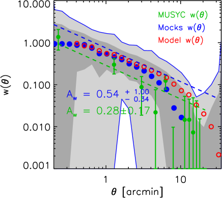
Figure 18: Angular clustering for the MUSYC Survey. Green circles show $w(\theta)$ calculated from the observed catalogue (Gawiser et al., 2007). The blue circles show the median $w(\theta)$ from all mock catalogues, with no correction for the integral constraint effect. The dark and light grey shaded regions respectively show the 68% and 95% ranges of the distribution of $w(\theta)$ measured in the mock catalogues. The red open circles show the Model correlation function, obtained using the width of the entire simulation box (and the same EW, flux and redshift limits). The dashed lines show the power-law fit to the observed $w(\theta)$ (green) and the median fit to $w(\theta)$ from the mock catalogues (blue). The amplitudes $A_{w}$ of these fits are also given in the figure.

References

- Ahn (2004) Ahn S-H., 2004, ApJ, 601, L25
- Ajiki et al. (2003) Ajiki M. et al., 2003, AJ, 126, 2091
- (3) Angulo R. E., Baugh C. M., Lacey C. G., 2008, MNRAS, 387, 921
- Atek et al. (2008) Atek, H., Kunth, D., Hayes, M., Ostlin, G., Mas-Hesse, J.M., 2008, A&A, 488, 491.
- Barton et al (2004) Barton, E.J., Dave, R., Smith, J-D.T., Papovich, C. Hernquist, L. Springel, V., 2004, ApJ, 604, 1
- Baugh et al. (1996) Baugh, C.M., Gardner J.P., Frenk C.S., Sharples R.M., 1996, MNRAS, 283, 15
- Baugh et al (2005) Baugh C.M., Lacey C.G., Frenk C.S., Granato G.L., Silva L., Bressan A., Benson A.J., Cole S., 2005, MNRAS, 356, 1191
- Baugh (2006) Baugh, C.M., 2006, Rep. Prog. Phys., 69, 3101
- Benson et al. (2000) Benson, A. J., Cole, S., Frenk, C. S., Baugh, C. M., Lacey, C. G., 2000, MNRAS, 311, 793
- Benson et al. (2002) Benson, A. J., Lacey, C. G., Baugh, C. M., Cole, S., & Frenk, C. S. 2002, MNRAS, 333, 156
- Berlind et al. (2002) Berlind A., Weinberg D., 2002, ApJ, 575, 587
- Berlind et al. (2003) Berlind A. A. et al., 2003, ApJ, 593, 1
- Cole et al (2000) Cole S., Lacey C.G., Baugh C.M., Frenk C.S., 2000, MNRAS, 319, 168
- Cooray & Sheth (2002) Cooray A., Sheth R., 2002, Phys. Rep., 372, 1
- Cowie & Hu (1998) Cowie L.L., Hu E.M, 1998, AJ, 115, 1319
- (16) Daddi E., Cimatti A., Pozzetti L., Hoekstra H., Röttgering H. J. A., Renzini A., Zamorani G., Mannucci F., 2000, A&A, 361, 535
- Davis & Peebles (1983) Davis M., Peebles P.J.E., 1983, ApJ, 267, 465
- Dunkley et al. (2008) Dunkley, J., et al., 2008, submitted to ApJS (arXiv:0803.0586)
- Ellis et al. (2001) Ellis R. S., Santos M. R., Kneib, J., Kuijken, K., 2001, ApJ, 560, 119
- Furlanetto et al (2005) Furlanetto, S.R., Schaye, J., Springel, V., Hernquist, L., 2005, ApJ, 622, 7
- Gao, Springel & White (2005) Gao L., Springel V., White S.D.M., 2005, MNRAS, 363, L66
- Gawiser et al. (2006) Gawiser E., et al., 2006, ApJS, 162, 1
- Gawiser et al. (2007) Gawiser E., et al., 2007, ApJ, 671, 278
- Gronwall et al. (2007) Gronwall C., et al., 2007, ApJ, 667, 79
- Haiman & Spaans (1999) Haiman, Z., Spaans, M., 1999, ApJ, 518, 138
- Hamana et al. (2004) Hamana T., Ouchi M., Shimasaku K., Kayo I., Suto Y., 2004, MNRAS, 347, 813
- Hayashino et al. (2004) Hayashino T., et al., 2004, AJ, 128, 2073
- Helly et al. (2003) Helly J., Cole S., Frenk C.S., Baugh C.M., Benson A., Lacey C., 2003, MNRAS, 338, 903
- Hewitt (1982) Hewitt P.C, 1982, MNRAS, 201, 867
- Hoeft et al. (2006) Hoeft M., Yepes G., Gottlöber S., Springel V., 2006, MNRAS, 371, 401
- Horton et al. (2004) Horton, A., Parry, I., Bland-Hawthorne, J., Cianci S., King D., McMahon R., Medlen S., 2004, SPIE, 5492, 1022
- Hu, Cowie & McMahon (1998) Hu E. M, Cowie L. L., McMahon R. G. 1998, ApJ, 502, L99
- Hu et al. (2004) Hu E.M., Cowie L.L., Capak P., McMahon R.G., Hayashino T., Komiyama Y., 2004, AJ, 127, 563
- Hughes et al. (1998) Hughes D.H., et al., 1998, Nature, 394, 241
- Iye et al. (2006) Iye, M., et al., 2006, Nature, 443, 186
- Kashikawa et al. (2006) Kashikawa N., et al., 2006, ApJ, 648,7
- Kennicut (1983) Kennicut R.C., 1983, MNRAS, 301, 569
- Kobayashi et al. (2007) Kobayashi M., Totani T., Nagashima M., 2007, ApJ, 670, 919
- Kogut et al. (2003) Kogut, A., et al. 2003, ApJS, 148, 161
- Kudritzki et al. (2000) Kudritzki R.-P. et al., 2000, ApJ, 536, 19
- Lacey & Cole (1993) Lacey C.G., Cole S., 1993, MNRAS, 262, 627
- Lacey et al. (2008) Lacey, C. G., Baugh, C. M., Frenk, C. S., Silva, L., Granato, G. L., & Bressan, A. 2008, MNRAS , 385, 1155
- Landy & Szalay (1993) Landy S., Szalay A., 1993, ApJ, 412, 64
- Laursen & Sommer-Larsen (2007) Laursen P., Sommer-Larsen J., 2007, ApJ, 657, L69
- Le Delliou et al. (2005) Le Delliou, M., Lacey, C., Baugh, C.M., Guiderdoni, B., Bacon, R., Courtois, H., Sousbie, T., Morris, S.L., 2005, MNRAS, 357, L11
- Le Delliou et al. (2006) Le Delliou, M., Lacey, C. G., Baugh, C. M., Morris, S. L., 2006, MNRAS, 365, L712
- Maier et al. (2003) Maier C. et al., 2003, A&A, 402, 79
- Mandelbaum et al. (2005) Mandelbaum R., Tasitsiomi A., Seljak U., Kravtsov A.V., Wechsler R.H., 2005, MNRAS, 362, 1451
- Mo & White (1996) Mo H.J., White S.D.M., 1996, MNRAS, 282, 347
- Nagamine et al. (2006) Nagamine K., Cen R., Furlanetto S., Hernquist L., Night C., Ostriker J.P., Ouchi M., 2006, NewAR, 50, 29
- Nagamine et al. (2008) Nagamine K., Ouchi M., Springel V., Hernquist L., 2008, astro-ph:08020228
- Nagashima et al. (2005a) Nagashima, M., Lacey, C. G., Baugh, C. M., Frenk, C. S., & Cole, S. 2005, MNRAS, 358, 1247
- Nagashima et al. (2005b) Nagashima, M., Lacey, C. G., Okamoto, T., Baugh, C. M., Frenk, C. S., & Cole, S. 2005, MNRAS, 363, L31
- Nilsson et al. (2007a) Nilsson K., Orsi A., Lacey C.G.L., Baugh C.M., 2007, A&A, 474, 385
- Nilsson et al. (2007b) Nilsson K., Fynbo J., Moller P., Orsi A., 2007, ASP Conf. Ser. Vol. 380, p.61
- Okamoto, Gao & Theuns (2008) Okamato, T., Gao, L., Theuns, T., 2008, MNRAS 390, 920
- Ouchi et al. (2005) Ouchi M., et al., 2005, ApJ, 620, 1
- Ouchi et al. (2007) Ouchi M., et al., 2007, astro-ph:07073161
- Osterbrock (1989) Osterbrock D.E.,1989, Astrophysics of Gaseous Nebulae and Active Galactic Nuclei. University Science Books, Mill Valley CA
- Peebles (1980) Peebles, P.J.E, 1980, The Large-Scale Structure of the Universe (Princeton: Princeton Univ. Press)
- Press & Schechter (1974) Press W., Schechter P., 1974, ApJ, 187, 425
- Quadri et al. (2007) Quadri R., et al., 2007, AJ, 134, 1103
- Rhoads et al. (2003) Rhoads J.E. et al., 2003, AJ, 125, 1006
- Santos et al. (2004) Santos M. R., Ellis R. S., Kneib J., Richard J., Kuijken K., 2004, ApJ, 606, 683
- Sheth, Mo & Tormen (2001) Sheth R. K., Mo H. J., Tormen G., 2001, MNRAS, 323, 1
- Shimazaku et al. (2004) Shimazaku K., et al., 2004, ApJ, 605, L93
- Shimasaku et al. (2006) Shimasaku, K. et al., 2006, PASJ, 58, 313
- Simon (2007) Simon, P. 2007, A&A, 473, 711
- Smail et al. (1997) Smail I., Ivison R.J., Blain A.W., 1997, ApJ, 490, 5
- Springel et al. (2005) Springel V. et al., 2005, Nature, 435, 639
- Stark et al. (2007) Stark D., Ellis R., Richard J., Kneib J., Smith G.P., Santos M., 2007, ApJ, 663,10
- Steidel et al. (1996) Steidel C.C., Giavalisco M., Pettini M., Dickinson M., Adelberger K., 1996, ApJ, 462, 17
- Steidel et al. (1999) Steidel C.C., Adelberger K., Giavalisco M., Dickinson M., Pettini M., 1999, ApJ, 519, 1
- Taniguchi et al. (2005) Taniguchi Y. et al., 2005, PASJ, 57, 165
- Tasitsiomi (2006) Tasitsiomi A., 2006, ApJ, 645, 792
- Verhamme et al. (2006) Verhamme A., Schaerer D., Maselli A., 2006, A&A, 460, 397
- Zheng & Miralda-Escudé (2002) Zheng Z., Miralda-Escude J., 2002, ApJ, 578, 33