Extracting synaptic conductances
from single membrane potential traces

Abstract

In awake animals, the activity of the cerebral cortex is highly complex, with neurons firing irregularly with apparent Poisson statistics. One way to characterize this complexity is to take advantage of the high interconnectivity of cerebral cortex and use intracellular recordings of cortical neurons, which contain information about the activity of thousands of other cortical neurons. Identifying the membrane potential (V_m) to a stochastic process enables the extraction of important statistical signatures of this complex synaptic activity. Typically, one estimates the total synaptic conductances (excitatory and inhibitory) but this type of estimation requires at least two V_m levels and therefore cannot be applied to single V_m traces. We propose here a method to extract excitatory and inhibitory conductances (mean and variance) from single V_m traces. This “VmT method” estimates conductance parameters using maximum likelihood criteria, under the assumption that synaptic conductances are described by Gaussian stochastic processes and are integrated by a passive leaky membrane. The method is illustrated using models and is tested on guinea-pig visual cortex neurons in vitro using dynamic-clamp experiments. The VmT method holds promises for extracting conductances from single-trial measurements, which has a high potential for in vivo applications.

In awake animals, neurons in different cortical structures display highly irregular spontaneous firing (Evarts, 1964; Steriade and McCarley, 1990). This level of firing must be considered together with the dense connectivity of cerebral cortex. Each pyramidal neuron receives between 5000 and 60000 synaptic contacts and a large part of this connectivity originates from the cortex itself (DeFelipe and Farinas, 1992; Braitenberg and Schüz, 1998). As a consequence, many synaptic inputs are simultaneously active onto cortical neurons in intact networks. Indeed, intracellular recordings in awake animals reveal that cortical neurons are subjected to an intense synaptic bombardment and, as a result, are depolarized and have a low input resistance (Matsumara et al., 1988; Baranyi et al., 1993; Steriade et al., 2001) compared to brain slices kept in vitro. This activity is also responsible for a considerable amount of subthreshold fluctuations, called “synaptic noise”. This noise level and its associated “high-conductance state” greatly affect the integrative properties of neurons (reviewed in Destexhe et al., 2003; Destexhe, 2007; Longtin, 2008).

To characterize this activity, one must use appropriate methods to measure not only the mean conductance level of excitatory and inhibitory inputs, but also their level of fluctuations which is quantified by the conductance variance. Many methods exist to extract mean conductances (see review by Monier et al., 2008), but few methods have been proposed to extract the variances. One class of methods consists of identifying the membrane potential (V_m) to a multidimensional stochastic process (Rudolph and Destexhe, 2003c, 2005). The so-called “VmD method” (Rudolph et al., 2004) enables the extraction of mean and variance of excitatory and inhibitory conductances. This method, however, requires to use at least two different levels of V_m activity, which prevents its application to single-trial measurements.

More recently, a related method was proposed to extract spike-triggered average conductances from the V_m (Pospischil et al., 2007). In this case, one needs to extract synaptic conductances time courses from a single trace (the spike-triggered V_m), which was made possible using a maximum likelihood method.

In the present paper, we attempt to merge these concepts and provide a method to estimate the excitatory and inhibitory conductances and their variances. This “VmT” method provides similar estimates as the VmD method, but it does so by using a maximum likelihood estimation, and thus can be applied to single V_m traces.

Experimental procedures

Models

All methods and analyses shown in this paper are based on a stochastic model of synaptic background activity, which was modeled by fluctuating conductances (Destexhe et al., 2001). In this model, the synaptic conductances are stochastic processes, which in turn influence V_m dynamics. According to this “point-conductance” model, the membrane potential dynamics is described by the following set of equations:

$$C\ \frac{dV}{dt} = -G_{L}\,(V-E_{L})-g_{e}\,(V-E_{e})-g_{i}\,(V-E_{i})+\,I_{ext}~{},$$ (1)

$$\frac{dg_{e}(t)}{dt} = -\frac{1}{\tau_{e}}\,[g_{e}(t)-g_{e0}]+\sqrt{\frac{2\sigma^{2}_{e}}{\tau_{e}}}\ \xi_{e}(t)~{},$$ (2)

$$\frac{dg_{i}(t)}{dt} = -\frac{1}{\tau_{i}}\,[g_{i}(t)-g_{i0}]+\sqrt{\frac{2\sigma^{2}_{i}}{\tau_{i}}}\ \xi_{i}(t)~{},$$ (3)

where $C$ denotes the membrane capacitance, $I_{ext}$ a stimulation current, $G_{L}$ the leak conductance and $E_{L}$ the leak reversal potential. $g_{e}(t)$ and $g_{i}(t)$ are stochastic excitatory and inhibitory conductances with respective reversal potentials $E_{e}$ and $E_{i}$. The excitatory synaptic conductance is described by Ornstein-Uhlenbeck stochastic processes (Eq. 2), where $g_{e0}$ and $\sigma^{2}_{e}$ are, respectively, the mean value and variance of the excitatory conductance, $\tau_{e}$ is the excitatory time constant, and $\xi_{e}(t)$ is a Gaussian white noise source with zero mean and unit standard deviation. The inhibitory conductance $g_{i}(t)$ is described by an equivalent equation (Eq. 3) with parameters $g_{i0}$, $\sigma^{2}_{i}$, $\tau_{i}$ and noise source $\xi_{i}(t)$. For details about Ornstein-Uhlenbeck stochastic processes, see the review by Gillespie (1996).

This model was simulated together with a leaky integrator mechanism with no spiking mechanism because the method only applies to subthreshold activity. All numerical simulations were performed in the NEURON simulation environment (Hines and Carnevale, 1997) and were run on PC-based workstations under the LINUX operating system.

Experiments

In vitro experiments were performed on 0.4 mm thick coronal or sagittal slices from the lateral portions of guinea-pig occipital cortex. Guinea-pigs, 4-12 weeks old (CPA, Olivet, France), were anesthetized with sodium pentobarbital (30 mg/kg). The slices were maintained in an interface style recording chamber at 33-35${\,}^{\circ}C$. Slices were prepared on a DSK microslicer (Ted Pella Inc., Redding, CA) in a slice solution in which the NaCl was replaced with sucrose while maintaining an osmolarity of 307 mOsm. During recording, the slices were incubated in slice solution containing (in mM): NaCl, 124; KCl, 2.5; MgSO₄, 1.2; NaHPO₄, 1.25; CaCl₂, 2; NaHCO₃, 26; dextrose, 10, and aerated with 95% O₂, 5% CO₂ to a final pH of 7.4. Intracellular recordings following two hours of recovery were performed in deep layers (layer IV, V and VI) in electrophysiologically identified regular spiking and intrinsically bursting cells. Electrodes for intracellular recordings were made on a Sutter Instruments P-87 micropipette puller from medium-walled glass (WPI, 1BF100) and beveled on a Sutter Instruments beveler (BV-10M). Micropipettes were filled with 1.2 to 2M potassium acetate and had resistances of 60-100 M$\Omega$ after beveling.

All research procedures concerning the experimental animals and their care adhered to the American Physiological Society’s Guiding Principles in the Care and Use of Animals, to the European Council Directive 86/609/EEC and to European Treaties series no. 123, and was also approved by the local ethics committee “Ile-de-France Sud” (certificate no. 05-003).

The dynamic-clamp technique (Robinson et al., 1993; Sharp et al., 1993) was used to inject computer-generated conductances in real neurons. Dynamic-clamp experiments were run using the hybrid RT-NEURON environment (Sadoc et al., 2009), which is a DSP-based system using a modified version of the NEURON simulation environment (Hines and Carnevale, 1997). The dynamic-clamp protocol was used to insert the fluctuating conductances underlying synaptic noise in cortical neurons using the point-conductance model, similar to a previous study (Destexhe et al., 2001). According to Eq. (1) above, the injected current is determined from the fluctuating conductances $g_{e}(t)$ and $g_{i}(t)$ as well as from the difference of the membrane voltage from the respective reversal potentials, $I_{DynClamp}=-g_{e}\big{(}V-E_{e}\big{)}-g_{i}\big{(}V-E_{i}\big{)}$. The contamination of the measured membrane voltage $V$ by electrode artifacts due to simultaneous current injection was avoided through the use of Active Electrode Compensation (AEC), a novel, high resolution digital on-line compensation technique (Brette et al. 2008).

Results

We present here a method for extracting conductances by associating the V_m to a stochastic process, and which uses maximum likelihood criteria to perform this extraction from single V_m traces. We first describe the method, then test it successively using computational models and real neurons in vitro.

The VmT method: extracting conductances from single V_m traces

The starting point of the method is to search for the “most likely” conductances parameters ( $g_{e0}$, $g_{i0}$, $\sigma_{e}$ and $\sigma_{i}$) that are compatible with an experimentally observed V_m trace. We start from the point-conductance model (Eqs. 1–3), which is discretized in time with a step-size $\Delta t$. Eq. 1 can then be solved for $g_{i}^{k}$, which gives:

$$g_{i}^{k}=-\frac{C}{V^{k}-E_{i}}\left\{\frac{V^{k}-E_{L}}{\tau_{L}}+\frac{g_{e}^{k}(V^{k}-E_{e})}{C}+\frac{V^{k+1}-V^{k}}{\Delta t}-\frac{I_{ext}}{C}\right\},$$ (4)

where $\tau_{L}=C/G_{L}$.

Since the series $V^{k}$ for the voltage trace is known, $g_{i}^{k}$ has become a function of $g_{e}^{k}$. In the same way, we solve Eqs. 2–3 for $\xi_{s}^{k}$, which have become Gaussian distributed random numbers,

$$\xi_{s}^{k}=\frac{1}{\sigma_{s}}\sqrt{\frac{\tau_{s}}{2\Delta t}}\left(g_{s}^{k+1}-g_{s}^{k}\Big{(}1-\frac{\Delta t}{\tau_{s}}\Big{)}-\frac{\Delta t}{\tau_{s}}g_{s0}\right),$$ (5)

where $s$ stands for $e,i$.

There is a continuum of combinations $\{g_{e}^{k+1},g_{i}^{k+1}\}$ that can advance the membrane potential from $V^{k+1}$ to $V^{k+2}$, each pair occurring with a probability

$$p^{k} := p(g_{e}^{k+1},g_{i}^{k+1}|g_{e}^{k},g_{i}^{k})=\frac{1}{2\pi}e^{-\frac{1}{2}(\xi_{e}^{k2}+\xi_{i}^{k2})}=\frac{1}{2\pi}e^{-\frac{1}{4\Delta t}X^{k}},$$ (6)

$$X^{k} = \frac{\tau_{e}}{\sigma_{e}^{2}}\left(g_{e}^{k+1}-g_{e}^{k}\Big{(}1-\frac{\Delta t}{\tau_{e}}\Big{)}-\frac{\Delta t}{\tau_{e}}g_{e0}\right)^{2}$$

$$+\frac{\tau_{i}}{\sigma_{i}^{2}}\left(g_{i}^{k+1}-g_{i}^{k}\Big{(}1-\frac{\Delta t}{\tau_{i}}\Big{)}-\frac{\Delta t}{\tau_{i}}g_{i0}\right)^{2}.$$

These expressions are identical to those derived previously for calculating spike-triggered averages (Pospischil et al., 2007), except that no implicit average is assumed here.

Thus, to go one step further in time, a continuum of pairs $(g_{e}^{k+1},g_{i}^{k+1})$ is possible in order to reach the (known) voltage $V^{k+2}$. The quantity $p^{k}$ assigns to all such pairs a probability of occurrence, depending on the previous pair, and the voltage history. Ultimately, it is the probability of occurrence of the appropriate random numbers $\xi_{e}^{k}$ and $\xi_{i}^{k}$ that relate the respective conductances at subsequent time steps. It is then straightforward to write down the probability $p$ for certain conductance series to occur, that reproduce the voltage time course. This is just the probability for successive conductance steps to occur, namely the product of the probabilities $p^{k}$:

$$p=\prod_{k=0}^{n-1}p^{k},$$ (8)

given initial conductances $g_{e}^{0}$, $g_{i}^{0}$. However, again, there is a continuum of conductance series

$$\{g_{e}^{l},g_{i}^{l}\}_{l=1,\ldots,n+1},$$

that are all compatible with the observed voltage trace. We define a likelihood function $f(V^{k},\theta)$, $\theta=(g_{e0},g_{i0},\sigma_{e},\sigma_{i})$, that takes into account all of them with appropriate weight. We thus integrate Eq. 8 over the unconstrained conductances $g_{e}^{k}$ and normalize by the volume of configuration space:

$$f(V^{k},\theta)=\frac{\int\prod_{k=0}^{n-1}dg_{e}^{k}\;p}{\int\prod_{k=0}^{n-1}dg_{e}^{k}\,dg_{i}^{k}\;p},$$ (9)

where only in the nominator $g_{i}^{k}$ has been replaced by Eq. 4. This expression reflects the likelihood that a specific voltage series $\{V^{k}\}$ occurs, normalized by the probability, that any trace occurs. The most likely parameters $\theta$ giving rise to $\{V^{k}\}$ are obtained by maximizing (or minimizing the negative of) $f(V^{k},\theta)$ using standard optimization schemes (Press et al., 2007).

Test of the VmT method using model data

We tested the method in detail in its applicability to voltage traces that were created using the same model (leaky integrator model). To this end, we performed simulations scanning the ($g_{e0},g_{i0}$)–plane, and subsequently tried to re-estimate the conductance parameters used, but only from the V_m activity. For each parameter set ($g_{e0},g_{i0}$, $\sigma_{e}$, $\sigma_{i}$) the method was applied to ten samples of 5000 data points (corresponding to 250 ms each) and the average was taken subsequently. The conductance standard deviations (SDs) were chosen to be one third of the respective mean values, other parameters were assumed to be known during re-estimation ($C=0.4$ nF, $g_{L}=13.44$ nS, $E_{L}=-80$ mV, $E_{e}$ = 0 mV, $E_{i}$ = -75 mV, $\tau_{e}=2.728$ ms, $\tau_{i}=10.49$ ms), the time step was $dt=0.05$ ms. Also, we assumed that the total conductance $g_{tot}$ was known – this is the inverse of the apparent input resistance, which is generally known. This assumption is not mandatory, but the estimation becomes more stable. The likelihood function given by Eq. 9 was thus only maximized with respect to $g_{e0},\sigma_{e}$ and $\sigma_{i}$. Fig. 1 summarizes the results obtained.

The mean conductances are well reproduced over the entire scan region. An exception is the estimation of $g_{i0}$ in the case where the mean excitation exceeds inhibition by several-fold, a situation which is rarely found in real neurons. The situation for the SDs is different. While the excitatory SD is reproduced very well in the whole area under consideration, this is not necessarily the case for inhibition. Here, the estimation is good for most parts of the scanned region, but shows a considerable deviation along the left and lower boundaries. These are regions where the transmembrane current due to inhibition is weak, either because the inhibitory conductance is weak (lower boundary) or because it is strong and excitation is weak (left boundary), such that the mean voltage is close to the inhibitory reversal potential and the driving force is small. In these conditions, it seems that the effect of inhibition on the membrane voltage cannot be distinguished from that of the leak conductance.

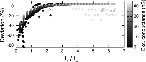
Figure 2: The estimation error depends on the ratio of inhibitory and leak conductances.

This point is illustrated in Fig. 2. The relative deviation between $\sigma_{i}$ in the model and its re-estimation depends on the ratio of the transmembrane current due to inhibitory ($I_{i}$) and leak ($I_{L}$) conductance. The estimation fails when the inhibitory current is smaller or comparable to the leak current, but it becomes very reliable as soon as the ratio $I_{i}/I_{L}$ becomes larger than 1.5–2. Some points, however, have large errors although with dominant inhibition. These points have strong excitatory conductances (see gray scale) and correspond to the upper right corner of Fig. 1D. The error is due to aberrant estimates for which the predicted variance is zero; in principle such estimates could be detected and discarded, but no such detection was attempted here. Besides these particular combinations, the majority of parameters with strong inhibitory conductances gave acceptable errors. We conclude that the estimation of the conductance variances will be most accurate in high-conductance states, where inhibitory conductances are strong and larger than the leak conductance.

Effect of recording noise

The unavoidable presence of recording noise may present a problem in the application of the method to recordings from real neurons. Fig. 3 (left) shows how low-amplitude white noise added to the voltage trace of a leaky integrator model impairs the reliability of the method. A Gaussian-distributed white noise was added to the voltage trace at every time step, scaled by the amplitude given in the abscissa. Different curves correspond to different pairs ($g_{e0}$, $g_{i0}$) colored as a function of the total conductance. The noise has an opposite effect on the estimation of the conductance mean values. While the estimate of excitation exceeds the real parameter value, for inhibition the situation is inverted. However, one has to keep in mind that both parameters are not estimated independently, but their sum is kept fixed. In contrast, the estimates for the conductance SDs always exceed the real values, and they can deviate by almost 500% for a noise amplitude of 10 $\mu$V. Here, the largest errors generally correspond to lowest conductance states. Clearly, in order to apply the method to recordings from real neurons, one needs to restrain this noise sensitivity.

Fortunately, this noise sensitivity can be reduced by standard noise reduction techniques. For example, preprocessing and smoothing the data using a Gaussian filter greatly diminishes the amplitude of the noise, and consequently improves the estimates according to the new noise amplitude (see Fig. 3, right panels). Too much smoothing, however, may result in altering the signal itself, and may introduce errors. It is therefore preferable to use smoothing at very short time scales (SD of 1–4 data points, depending on the sampling rate). In the next sections, we preprocessed the experimental voltage traces with a Gaussian filter with a SD of 3 data points.

Application of the VmT method to in vitro data

We next tested the method on in vitro recordings (n=5 cortical neurons, 17 injections) using dynamic clamp experiments (Fig. 4). As in the model, the stimulus consisted of two channels of fluctuating conductances representing excitation and inhibition. The conductance injection spanned values from low-conductance (of the order of 5-10 nS) to high-conductance states (50-160 nS). It is apparent from Fig. 4 that the mean values of the conductances ($g_{e0}$, $g_{i0}$) are well estimated, as expected because the total conductance is known in this case.

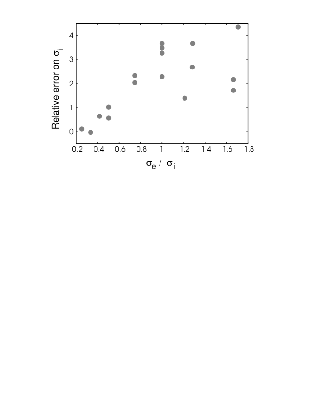
Figure 5: Relative error on inhibitory variance is high only when excitatory fluctuations dominate.

However, the estimation is subject to larger errors for the standard deviations of the conductances ($\sigma_{e}$, $\sigma_{i}$). In addition, the error on estimating variances is also linked to the accuracy of the estimates of synaptic time constants $\tau_{e}$ and $\tau_{i}$, similar to the VmD method (see discussion in Piwkowska et al., 2008). Interestingly, for some cases, the estimation works quite well (see indexed symbols in Fig. 4). In the pool of injections, there are three cases that represent a cell in a high-conductance state, i.e. the mean inhibitory conductances are roughly three times greater than the excitatory ones, and the standard deviations obey a similar ratio. For these trials, the estimate comes close to the values used during the experiment. Indeed, we found that the relative error on $\sigma_{i}$ is roughly proportional to the ratio $\sigma_{e}/\sigma_{i}$ for ratios smaller than 1, and tends to saturate for larger ratios (Fig. 5). In other words, the estimation has the lowest errors when inhibitory fluctuations dominate excitatory fluctuations. A recent estimate of conductance variances in cortical neurons of awake cats reported that $\sigma_{i}$ is larger than $\sigma_{e}$ for the vast majority of cells analyzed (Rudolph et al., 2007). The same was also true for anesthetized states (Rudolph et al., 2005), suggesting that the VmT method should give acceptable errors in practical situations in vivo.

Discussion

In this paper, we have introduced and tested a new method to estimate conductance mean and variance from single V_m traces. Traditional methods to estimate conductances require to perform current-clamp or voltage-clamp recordings at different voltages (Rudolph et al., 2004; Monier et al., 2008). If the membrane has intrinsic voltage-dependent conductances, the use of different voltage levels will necessarily cause important errors. This is particularly critical in vivo, where pharmacological manipulations to suppress currents are usually very limited.

Several methods exists that can be applied to single V_m traces; for example, one can calculate power spectral densities (PSD) of the V_m. The fitting of analytical expressions of the V_m PSD would allow in principle to estimate the conductance parameters, since they appear in these expressions. However, this analysis would require to know the effective membrane time constant, and therefore the total conductance. In such a case, since the average V_m is known, the conductances can be estimated by simply solving the membrane equation at steady-state, so the PSD presents no useful means of estimating conductances. Nevertheless, fitting theoretical expressions to experimental PSDs can in principle yield estimates of other parameters, such as the decay time constants of synaptic conductances, although such estimates can be subject to important errors (see Piwkowska et al., 2008 for an assessment of this method).

A second type of method applicable to single V_m traces is to estimate the spike-triggered average (STA) of synaptic conductances (Pospischil et al., 2007). The principle of this method is to search for the most probable conductance traces that account for the V_m STA. These traces are calculated by maximum likelihood following a discretization of the time axis. The performance of this method was tested using computational models and dynamic-clamp experiments (Pospischil et al., 2007; Piwkowska et al., 2008). It was found to be excellent, and the STA method was applied to estimate the optimal conductance patterns preceding spikes in vivo (Rudolph et al., 2007). However, this method requires a prior knowledge of the conductance parameters ($g_{e0}$, $g_{i0}$, $\sigma_{e}$, $\sigma_{i}$). In practice, it is thus necessary to apply the VmD method beforehand, which in turn requires recording at several V_m levels.

We proposed here a method that merges the above concepts. The VmT method can estimate the same conductance parameters as the VmD method ($g_{e0}$, $g_{i0}$, $\sigma_{e}$, $\sigma_{i}$), but using a maximum likelihood approach similar to the STA estimates. The analysis can thus be realized from single V_m levels, thereby limiting the bias caused by voltage-dependent currents. The VmT method does not rely on static properties of the membrane voltage, like mean and standard deviation, in order to determine the shape of the conductance distributions. Instead, it exploits the dynamical information hidden in the V_m time course. Not only the step sizes $\Delta t$ are important, but also at which voltage level they occur. The likelihood function is highly sensitive to the conductance fluctuations and, constraining the total conductance, also to the conductance mean values.

A word of caution is needed here about the biological significance of the conductances estimated by the VmT method. Like any other method to extract conductances from V_m activity, the conductance estimated here refers to the conductance visible at the site of the V_m recording, in general the soma. This somatic conductance can be very different – and is in general smaller – than the conductance present at the site of the synaptic receptors, mostly the dendrites. This is especially critical for neurons with extended dendritic morphologies, such as pyramidal neurons, which experience considerable dendritic attenuation. However, the visible somatic conductances are close to the conductances participating to the interactions involved in generating the action potential, because the region for spike initiation (presumably the initial part of the axon; see review by Stuart et al., 1997) is electrotonically close to the soma. To yield estimates closer to the conductances present in dendrites, recordings must be done using drugs such as QX-314 and cesium, to reduce the leak conductance and thereby lead to more compact neurons, with more limited dendritic attenuation. The conductance contribution due to spikes (somatic or dendritic) should be avoided by using exclusively subthreshold activity.

Similarly, like all other methods for the analysis of synaptic conductances, the VmT method rests on the assumption that the range of V_m analyzed is linear, and does not contain voltage-dependent conductances. Nevertheless, it is possible to follow a similar maximum-likelihood procedure by explicitly including fast voltage-dependent conductances in the model. The VmT method also requires knowledge of the passive parameters of the recorded neuron ($G_{L}$, $C$…) which may be difficult to obtain in vivo (see Piwkowska et al., 2008 for a discussion of this point).

A second word of caution concerns the significance of conductance variances. The conductance variances estimated using the VmT method are specific to the “point-conductance” model, in which the V_m activity is assumed to result from the action of two stochastic synaptic conductances (Destexhe et al., 2001). In particular, one of the assumptions was that the excitatory and inhibitory conductances are Gaussian-distributed. Estimates of variances of course depend on this assumption. Including asymmetric conductance distributions is possible but would substantially complicate the model. The mathematical simplicity of this model has made it possible to design a series of methods to analyze the V_m activity (reviewed in Piwkowska et al., 2008). The VmT method is a natural extension of this approach.

The tests of the VmT method on model data were encouraging, but also pointed to weaknesses of the method in a regime where the transmembrane current due to inhibitory conductances is small compared to the leak current. In this case, the inhibitory fluctuations are not reliably resolved. Furthermore, the presence of recording noise can disturb the estimation significantly. Though smoothing the voltage trace could in some cases re-establish a good result (Fig. 3), more sophisticated procedures should be considered to eliminate this sensitivity to noise. For example, one could introduce to Eq. 1 an additive noise term, whose SD would become an additional parameter that has to be estimated. Thus, in principle, if this weak inhibition regime can be avoided, the VmT method should be applicable to real neurons. In any case, to be on the safe side, it is preferable to use the VmT method on V_m traces with the lowest possible level of instrumental noise.

We also tested the VmT method by using dynamic-clamp injection of stochastic conductances. In this case, controlled conductances are injected while the V_m activity is being recorded, allowing to compare the VmT estimates from the V_m, to the conductances actually injected. These tests confirmed the weakness of the method in the low-inhibition regime, but also revealed a good performance of the VmT method during HC states. Since in cortical neurons in vivo the membrane potential is usually well above the inhibitory reversal potential, and since inhibitory conductances tend to dominate over excitatory ones (Borg-Graham et al., 1998; Rudolph et al., 2007; note that dendritic recordings may be dominated by excitatory inputs), we anticipate that this method should provide good conductance estimates from in vivo recordings.

Acknowledgments

This research was supported by the Centre National de la Recherche Scientifique (CNRS, France), the Agence Nationale de la Recherche (ANR, France), Future and Emerging Technologies (FET, European Union) and the Human Frontier Science Program (HFSP). Additional information is available at http://cns.iaf.cnrs-gif.fr

References

1. Baranyi A, Szente MB, Woody CD. (1993) Electrophysiological characterization of different types of neurons recorded in vivo in the motor cortex of the cat. II. Membrane parameters, action potentials, current-induced voltage responses and electrotonic structures. J. Neurophysiol. 69: 1865-1879.

2. Borg-Graham, L.J., Monier, C., Frégnac, Y. (1998) Visual input evokes transient and strong shunting inhibition in visual cortical neurons. Nature 393: 369-373.

3. Braitenberg, V., Schüz, A. (1998) Cortex: statistics and geometry of neuronal connectivity (2nd edition), Springer-Verlag, Berlin.

4. Brette R, Piwkowska Z, Monier C, Rudolph-Lilith M, Fournier J, Levy M, Frégnac Y, Bal T, Destexhe A (2008) High-resolution intracellular recordings using a real-time computational model of the electrode. Neuron 59: 379-391.

5. DeFelipe, J., Fariñas, I. (1992) The pyramidal neuron of the cerebral cortex: morphological and chemical characteristics of the synaptic inputs. Prog. Neurobiol. 39: 563-607.

6. Destexhe, A. (2007) High-conductance state. Scholarpedia 2(11): 1341
   http://www.scholarpedia.org/article/High-Conductance_State

7. Destexhe A, Rudolph M, Fellous J-M, Sejnowski TJ. (2001) Fluctuating synaptic conductances recreate in-vivo–like activity in neocortical neurons. Neuroscience 107: 13-24.

8. Destexhe A, Rudolph, M, Paré D (2003) The high-conductance state of neocortical neurons in vivo. Nature Reviews Neurosci. 4: 739-751.

9. Evarts, E.V. (1964) Temporal patterns of discharge of pyramidal tract neurons during sleep and waking in the monkey. J. Neurophysiol. 27: 152-171.

10. Gillespie, D.T. (1996) The mathematics of Brownian motion and Johnson noise. Am. J. Phys. 64: 225-240.

Figures

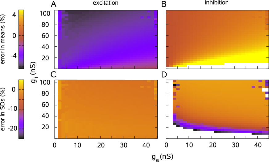
Figure 1: Test of the single-trace VmT method using a leaky integrator model.

Each panel presents a scan in the ($g_{e0},g_{i0}$)–plane. Color codes the relative deviation between model parameters and their estimates using the method (note the different scales for means/SDs). The white areas indicate regions where the mismatch was larger, $>$5% for the means and $<$-25% for SDs. A. Deviation in the mean of excitatory conductance ($g_{e0}$). B. Same as A, but for inhibition. C. Deviation in the SD of excitatory conductance. D. Same as C, but for inhibition. In general the method works well, except for a small band for the inhibitory SD.

The relative deviation between the parameter $\sigma_{i}$ in the simulations and its re-estimated value is shown as a function of the ratio of the currents due to inhibitory and leak conductances. The estimation fails when the inhibitory component becomes too small. The same data as in Fig. 1 are plotted: different dots correspond to different pairs of excitatory and inhibitory conductances ($g_{e0}$, $g_{i0}$), and the dots are colored according to the excitatory conductance (see scale). Details about the duration of injections etc. are given in the text.

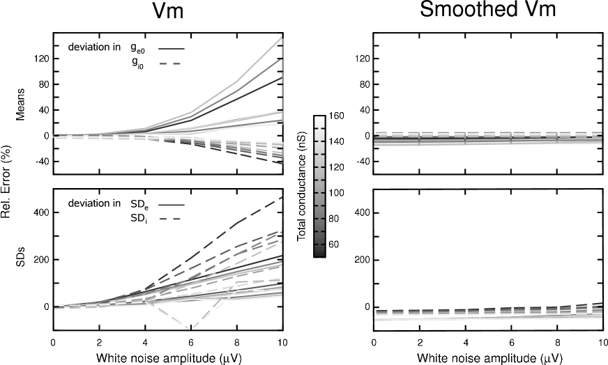
Figure 3: Error of the VmT estimates following addition of white noise to the voltage trace.

Gaussian white noise was added to the voltage trace of the model, and the VmT method was applied to the V_m trace obtained with noise, to yield estimates of conductances and variances. Left: relative error obtained in the estimation of $g_{e0}$ and $g_{i0}$ (upper panel), as well as $\sigma_{e}$ and $\sigma_{i}$ (lower panels). Right: same estimation, but the V_m was smoothed prior to the VmT estimate (Gaussian filter with SD of 1 data point). In both cases, the relative error is shown as a function of the white noise amplitude. Different curves correspond to different pairs ($g_{e0}$, $g_{i0}$). The errors on the estimates for both mean conductance and SD increase with the noise. The coloring of the curves as a function of the total conductance (see scale) shows that the largest errors generally occur for the low-conductance regimes. The error was greatly diminished by smoothing (right panels).

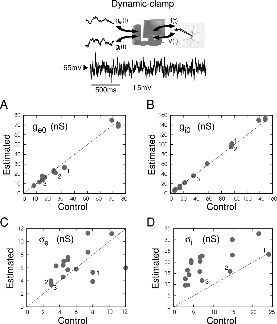
Figure 4: Dynamic-clamp test of the VmT method to extract conductances from guinea-pig visual cortical neurons in vitro.

Fluctuating conductances of known parameters were injected in different neurons using dynamic-clamp, and the V_m activity produced was analyzed using the single-trace VmT method. Each plot represents the different conductance parameters extracted from the V_m activity: $g_{e0}$ (A), $g_{i0}$ (B), $\sigma_{e}$ (C) and $\sigma_{i}$ (D). The extracted parameter (Estimated) is compared to the value used in the conductance injection (Control). While in general the mean conductances are matched very well, the estimated SDs show a large spread around the target values. Nevertheless, during states dominated by inhibition (see indexed symbols), the estimation was acceptable.

The relative mean-square error on $\sigma_{i}$ is represented as a function of the $\sigma_{e}/\sigma_{i}$ ratio. The error is approximately proportional to the ratio of variances. The same data as in Fig. 4 were used.

References

- [1] Hines, M.L. and N.T. Carnevale. (1997) The NEURON simulation environment. Neural Computation 9: 1179-1209.
- [2]
- [3] Longtin, A. (2008) Neuronal noise. Scholarpedia (in press)
- [4] http://www.scholarpedia.org/article/Neuronal_noise
- [5]
- [6] Matsumara M, Cope T, Fetz EE. (1988) Sustained excitatory synaptic input to motor cortex neurons in awake animals revealed by intracellular recording of membrane potentials. Exp. Brain Res. 70: 463-469.
- [7]
- [8] Monier C, Fournier J, Frégnac Y. (2008) In vitro and in vivo measures of evoked excitatory and inhibitory conductance dynamics in sensory cortices. J. Neurosci. Meth. (in press)
- [9]
- [10] Piwkowska, Z., Pospischil, M., Brette, R., Sliwa, J., Rudolph-Lilith, M., Bal, T., Destexhe, A. (2008) Characterizing synaptic conductance fluctuations in cortical neurons and their influence on spike generation. J. Neurosci. Methods 169: 302-322.
- [11]
- [12] Pospischil M, Piwkowska Z, Rudolph M, Bal T, Destexhe A. (2007) Calculating event-triggered average synaptic conductances from the membrane potential. J. Neurophysiol. 97: 2544-2552.
- [13]
- [14] Press W.H., Flannery B.P., Teukolsky S.A., Vetterling W.T. (2007) Numerical Recipes: The Art of Scientific Computing (3rd edition). Cambridge University Press, Cambridge UK.
- [15]
- [16] Robinson H.P. and Kawai N. (1993) Injection of digitally synthesized synaptic conductance transients to measure the integrative properties of neurons. J. Neurosci. Methods 49: 157-165.
- [17]
- [18] Rudolph M, Destexhe A. (2003c) Characterization of subthreshold voltage fluctuations in neuronal membranes. Neural Computation 15: 2577-2618.
- [19]
- [20] Rudolph M, Destexhe A. (2005) An extended analytic expression for the membrane potential distribution of conductance-based synaptic noise. Neural Computation 17: 2301-2315.
- [21]
- [22] Rudolph M, Piwkowska Z, Badoual M, Bal T, Destexhe A. (2004) A method to estimate synaptic conductances from membrane potential fluctuations. J. Neurophysiol. 91: 2884-2896.
- [23]
- [24] Rudolph, M., Pelletier, J-G., Paré, D. and Destexhe, A. (2005) Characterization of synaptic conductances and integrative properties during electrically-induced EEG-activated states in neocortical neurons in vivo. J. Neurophysiol. 94: 2805-2821.
- [25]
- [26] Rudolph M, Pospischil M, Timofeev I, Destexhe A. (2007) Inhibition controls action potential generation in awake and sleeping cat cortex. J Neurosci. 27: 5280-5290.
- [27]
- [28] Sadoc G, Le Masson G, Foutry B, Le Franc Y, Piwkowska Z, Destexhe A and Bal T. (2009) Recreating in vivo–like activity and investigating the signal transfer capabilities of neurons: Dynamic-clamp applications using real-time NEURON. In: Dynamic-clamp: From Principles to Applications, Edited by Destexhe A and Bal T, Springer, new York, in press.
- [29] Sharp, A.A., O’Neil, M.B., Abbott, L.F. and Marder, E. (1993) The dynamic clamp: artificial conductances in biological neurons. Trends Neurosci. 16: 389-394.
- [30] Steriade, M., McCarley, R.W. (1990) Brainstem Control of Wakefulness and Sleep, Plenum Press, New York.
- [31] Steriade M, Timofeev I, Grenier F. (2001) Natural waking and sleep states: a view from inside neocortical neurons. J. Neurophysiol. 85: 1969-1985.
- [32] Stuart, G., Spruston, N., Sakmann, B. and Hausser, M. (1997) Action potential initiation and backpropagation in neurons of the mammalian CNS. Trends Neurosci. 20: 125-131.