Singularities in Speckled Speckle: Screening

Abstract

We study screening of optical singularities in random optical fields with two widely different length scales.  We call the speckle patterns generated by such fields speckled speckle, because the major speckle spots in the pattern are themselves highly speckled.  We study combinations of fields whose components exhibit short- and long-range correlations, and find unusual forms of screening.

I INTRODUCTION

Screening of charged topological singularities - vortices [1, 2 (Chap. 5), $3$ (Sect. $4.8$)] in scalar fields, C points [$2,$ (Chaps. $12$ and $13$)] in vector fields - has been extensively studied in random fields with a single correlation length [$4-19$]; here we study screening of these singularities in random fields with two widely different correlation lengths.  We call such fields “speckled speckle” because, as illustrated in Fig. 1(a), the major speckle spots of the field are themselves highly speckled.  Speckled speckle fields can be generated by illuminating a random diffuser with two concentric, overlapping beams: one, the $a$ beam, is tightly focused and intense, the other, the $b$ beam, is weak and diffuse.

The statistical properties of speckled speckle can be highly anomalous, with relative number densities of critical points (vortices, C points, extrema, and umbilic points) differing from normal  speckle values by orders of magnitude [$20,21$]. The spatial arrangement of vortices and C points is also anomalous, with these singularities forming dense clusters of a kind not found in normal speckle fields, Fig. 1(a) [$20,21$].

Screening can be either short- or long-ranged.  Nonsingular random sources produce random fields that exhibit short range screening [$4-19$].  In such systems positive (negative) topological charges are surrounded by a local net excess of negative (positive) charge, leading to charge neutrality within a characteristic distance, the screening length, that can be less than the average separation between charges [$19$].

Singular sources, such as a ring of finite radius but zero width [$8$], produce random fields that exhibits long-range screening [$8,16,19$].  The singularities in the field produced by a ring form a quasi-lattice in which positive/negative singularities occupy alternate corners of a square cell, Fig. 1(b).  Local defects in the lattice destroy the local charge neutrality that would produce short range screening, and screening sets in only asymptotically.

Thus, both short- and long-range screening depend upon the spatial arrangements of the charges.  These arrangements are anomalous in speckled speckle, which can therefore be expected to exhibit unusual forms of screening.

A major observable consequence of screening is strong damping of fluctuations of the topological charge $Q$.  These fluctuations are characterized by their variance $\left\langle Q^{2}\right\rangle$; the behavior of $\left\langle Q^{2}\right\rangle$ for speckled speckle is our main concern here.

The plan of this paper is as follows.  In Section II we discuss the charge variance in a bounded region, in Section III we review $\left\langle Q^{2}\right\rangle$ in normal speckle for fields with short- and with long-range correlations, and in Sections IV-VII we present results for $\left\langle Q^{2}\right\rangle$ for four qualitatively different forms of speckled speckle.  We briefly summarize our main findings in the concluding Section VIII.

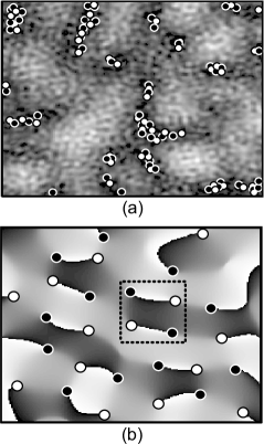
Figure 1: Vortex structures.  Positive (negative) vortices are shown by white (black) filled circles.  (a) Speckled speckle.  A random diffuser is illuminated by two concentric disks of light, $a$ and $b$.  The diameter of disk $b$ is ten times the diameter of $a$; the total optical power in $a$, however, is $10$ times that in $b$.  Major (minor) speckle spots in the speckled speckle field are due primarily to beam $a$ ($b$).  Vortices of the combined beam cluster in the dark regions between $a$ field speckle spots because they require perfect destructive interference between the strong $a$ and weak $b$ fields.  In normal speckle produced by a single disk vortices tend to be uniformly distributed with only minor clustering.  (b) Normal speckle phase map produced by a random diffuser illuminated with a single ring; the vortices tend to form a lattice with a square unit cell.

II CHARGE VARIANCE IN SHORT- AND LONG-RANGE SCREENING

We assume isotropy, circular Gaussian statistics [$3$ (Chap 2), $22$ (Chap. $2$)], and a circular region of radius $R$.  The charge variance $\left\langle Q^{2}\right\rangle$ in this region is related to the autocorrelation function of the field $W(r)$ by [$19$ (Eq. 39)],

$$\langle Q^{2}\rangle=\frac{1}{2\pi}\int_{0}^{2R}\sqrt{4R^{2}-r^{2}}\frac{(W^{\prime}(r))^{2}}{1-W^{2}(r)}dr.$$ (1)

where $W^{\prime}(r)=dW(r)/dr$.  The number density of charges $\eta$ is [$23$]

$$\eta=-\frac{W^{\prime\prime}(0)}{2\pi}.$$ (2)

For the short range correlations produced by extended sources, $W^{\prime}(r)$ decays rapidly with $r$, and in the limit of large $R$,

$$\langle Q^{2}\rangle\approx\frac{R}{\pi}\int_{0}^{\infty}\frac{(W^{\prime}(r))^{2}}{1-W^{2}(r)}dr.$$ (3)

Thus, for short-range screening $\left\langle Q^{2}\right\rangle$ grows with the perimeter, i.e. $\left\langle Q^{2}\right\rangle\sim R\sim\sqrt{N}$, in contrast to the case of no screening, where $\left\langle Q^{2}\right\rangle$ grows with the area, $\left\langle Q^{2}\right\rangle\sim R^{2}\sim N$ [$8,19$].

For the long-range screening produced by a singular ring source of radius $p$ and zero width, the large $R$ limit is [$19$ (Eq. 48)],

$$\left\langle Q^{2}\right\rangle \approx\dfrac{pR}{\pi^{2}}\left[{\cal{K}}+\ln\left(\rho R\right)\right],$$ (4a)

$${\cal{K}} =\pi{\cal{D}}+\gamma+5\ln 2-3\approx 2.81182,$$ (4b)

$${\cal{D}} =\int_{0}^{\infty}dx\,\frac{J_{0}^{2}(x)J_{1}^{2}(x)}{1-J_{0}^{2}(x)}\approx 0.563047,$$ (4c)

where $$\gamma\approx 0.577216 R\ln R R R^{2} 10^{4} \sim 100 \sim 22$$ is Euler’s constant.  Thus, long-range screening yields a charge variance that grows asymptotically as ; this growth rate is significantly faster than the short-range growth rate proportional to , but is very much slower than the unscreened rate proportional to .  For, say, a large region that contains charges, short-range (long-range) screening damps out charge fluctuations relative to no screening by a factor of ().

III CHARGE VARIANCE IN NORMAL SPECKLE

We review here the charge variance in normal speckle produced by sources with a single characteristic length scale.  In later sections we build our composite sources with their two different length scales from binary combinations of these single sources, and compare composite-source charge variances with single-source variances.

III.1 Source Distributions and Autocorrelation Functions

Listed below are the source distributions $S(u)$, where $u$ measures radial displacements in the source plane, the total optical power in each source, $P$, and the autocorrelation functions $W(r)$ of the speckle field.  $S(u)$ and $W(r)$ are related by the VanCittert-Zernike theorem [$3$ (Sect. 4), $22$ (Sect. 5.6)].  We study four fields with autocorrelation functions that decay at different rates.

(i) A Gaussian, superscript (G), of $1/e$ width $p$, and intensity (optical power/unit area) $I^{\left(\text{G}\right)}$ at the peak; henceforth the “Gaussian”,

$$S^{\left(\text{G}\right)}(u) =I^{\left(\text{G}\right)}\exp\left(-\left[u/\left(2p\right)\right]^{2}\right),$$ (5a)

$$P^{\left(\text{G}\right)} =4\pi p^{2}I^{\left(\text{G}\right)},$$ (5b)

$$W^{(\text{G})}(r) =\exp\left(-p^{2}r^{2}\right).$$ (5c)

(ii) A uniform disk, superscript (D), of radius $p$, and uniform intensity $I^{\left(\text{D}\right)}$; henceforth the “Disk”,

$$S^{\left(\text{D}\right)}(u) =I^{\left(\text{D}\right)}\Theta\left(u-p\right),$$ (6a)

$$P^{\left(\text{D}\right)} =\pi p^{2}I^{\left(\text{D}\right)},$$ (6b)

$$W^{\left(\text{D}\right)}(r) =2J_{1}\left(pr\right)/\left(pr\right).$$ (6c)

$$\Theta\left(x\right) \Theta\left(x\leq 0\right)=0 \Theta\left(x>0\right)=1$$ is the Heaviside step function defined by , .

(iii) A nonuniform (inverse square root) disk, superscript (S), of radius $p$, with intensity $I^{\left(\text{S}\right)}$ at the disk center,

$$S^{\left(\text{S}\right)}\left(u\right) =\frac{I^{\left(\text{S}\right)}}{\sqrt{1-\left(u/p\right)^{2}}}\Theta\left(u-p\right),$$ (7a)

$$P^{\left(\text{S}\right)} =2\pi p^{2}I^{\left(\text{S}\right)},$$ (7b)

$$W^{\left(\text{S}\right)}(r) =I^{\left(\text{S}\right)}\text{sinc}\left(pr\right),$$ (7c)

where, sinc$$\left(x\right)\equiv\sin\left(x\right)/x$$.  In what follows we refer to this source as the “Sinc”.

(iv) A singular ring, superscript (R), of radius $p$, which we write as

$$S^{\left(\text{R}\right)}(u) =I^{\left(\text{R}\right)}\varepsilon\delta\left(u-p\right),$$ (8a)

$$P^{\left(\text{R}\right)} =2\pi p\varepsilon I^{\left(\text{R}\right)},$$ (8b)

$$W^{\left(\text{R}\right)}(r) =J_{0}(pr),$$ (8c)

where $$\delta\left(x\right)$$ is the Dirac delta function.  In what follows we refer to this source as the “Ring”.

$S^{\left(\text{R}\right)}(u)$ is the limit of a finite width annulus $s^{\left(\text{R}\right)}\left(u\right)$ of mean radius $p$ and width $\varepsilon$,

$$s\left(u\right)=\Theta\left(u-p-\varepsilon/2\right)-\Theta\left(u-p+\varepsilon/2\right),$$ (9a)

$$\lim_{\varepsilon\rightarrow 0}\left[s\left(u\right)/\varepsilon\right]=\delta\left(u-p\right).$$ (9b)

$$I^{\left(\text{R}\right)} \varepsilon\rightarrow 0 I^{\left(\text{R}\right)} P^{\left(\text{R}\right)}$$ is therefore the uniform intensity in the annulus.  In the limit , diverges, in Eq. (8b), however, is assumed to remain finite.

$W$ and $\left\langle Q^{2}\right\rangle$ for the finite width annulus $\left(\varepsilon>0\right)$ is discussed in [$19$ (Sect. 5)], where it is shown that over the region $\varepsilon r<1$ the experimentally attainable annulus is an excellent approximation to the theoretical singular ring.

III.2 Charge Variance

In Fig. 2 we plot $\left\langle Q^{2}\right\rangle/\left(pR\right)$ vs. $pR$ for the above four sources.  For the Gaussian (G), Disk (D), and Sinc (S), screening is short-ranged, and the large $R$ limit of $\left\langle Q^{2}\right\rangle$ is given in Eq. (3).

For the Gaussian, Eq. (3) can be evaluated analytically, yielding

$$\left\langle Q^{2}\right\rangle_{Gauss}\approx\tfrac{1}{4}\sqrt{2/\pi}\zeta\left(3/2\right)pR=0.521093pR,$$ (10)

with $\zeta\left(x\right)$ is the Riemann zeta function, whereas for the Disk (D) and Sinc (S), Eq. (3) is evaluated numerically, yielding

$$\left\langle Q^{2}\right\rangle_{Disk}\approx 0.227210pR,$$ (11)

and

$$\left\langle Q^{2}\right\rangle_{\operatorname{Si}nc}\approx 0.305898pR.$$ (12)

For the Ring (R) screening is long-ranged, and the large $R$ limit of $\left\langle Q^{2}\right\rangle/\left(pR\right)$ is given in Eq. (4).

For very small $R$ for all sources [$19$ (Eq. 82)],

$$\left\langle Q^{2}\right\rangle_{R\rightarrow 0}\approx\eta\pi R^{2}=N,$$ (13)

i.e. there is no screening; the reason is that for a sufficiently small area the probability of finding the required screening charges within the area is vanishingly small.  This result is illustrated in Fig. 2(c) for all four sources.

Figure 2: Charge variance $\left\langle Q^{2}\right\rangle$ for normal speckle obtained from numerical integration of Eq. (1).  (a) Short-range screening.  (b) Long-range screening.  The dependence on the parameter $p$ in Eqs. (5)-(8) is here scaled out by plotting $\left\langle Q^{2}\right\rangle/\left(pR\right)$ vs. $pR$.  As can be seen, for $pR>1$, the results in (a) quickly asymptote to the theoretical values in Eqs. (10)-(12), whereas the result in (b) asymptotes to the theoretical form (thin straight line) in Eq. (4).  (c) $\left\langle Q^{2}\right\rangle$ for small $R$.  In all four cases (G - Gauss, D - Disk, S - Sinc, and R - Ring), the curves approach the $R\rightarrow 0$ limit given in Eq. (13).

IV COMPOSITE SOURCES AND THEIR AUTOCORRELATION FUNCTIONS

For scalar (single component) fields the $a$ and $b$ beams have the same, say, linear polarization, and the singularities whose screening is of interest here are the phase vortices [$1-19$].  For vector (two component) fields the $a$ and $b$ beams have orthogonal linear polarizations, and the relevant singularities that screen each other are either right- or left-handed C points [$2$]: right-handed C points do not screen left-handed ones, and vice versa.

We write our composite source as

$$S^{\left(\text{T}_{a}\text{T}_{b}\right)}\left(u\right)=S_{a}^{\left(\text{T}\right)}\left(u\right)+S_{b}^{\left(\text{T}\right)}\left(u\right),$$ (14)

where the source type specifier $\left(\text{T}_{a}\text{T}_{b}\right)$ is a binary combination of T${}_{a,b}=$ G, D ,S, R.  From the VanCittert-Zernike theorem, the corresponding autocorrelation function is

$$W^{\left(\text{T}_{a}\text{T}_{b}\right)}(r)=\frac{W_{a}^{\left(\text{T}\right)}\left(r\right)+K^{\left(\text{T}_{a}\text{T}_{b}\right)}W_{b}^{\left(\text{T}\right)}\left(r\right)}{1+K^{\left(\text{T}_{a}\text{T}_{b}\right)}},$$ (15)

where the dimensionless constant

$$K^{\left(\text{T}_{a}\text{T}_{b}\right)}=P_{b}^{\left(\text{T}\right)}/P_{a}^{\left(\text{T}\right)}.$$ (16)

$S_{a,b}^{\left(\text{T}\right)}(u)$, $P_{a,b}^{\left(\text{T}\right)}$, and $W_{a,b}^{\left(\text{T}\right)}\left(r\right)$, are listed in Eqs. (5)-(8), with $p=a,b$ as appropriate.

Similarly, the number density of singularities is for composite scalar fields,

$$\eta^{\left(\text{T}_{a}\text{T}_{b}\right)}=-\frac{1}{2\pi}\frac{W_{a}^{\prime\prime\left(\text{T}\right)}(0)+K^{\left(\text{T}_{a}\text{T}_{b}\right)}W_{b}^{\prime\prime\left(\text{T}\right)}(0)}{1+K^{\left(\text{T}_{a}\text{T}_{b}\right)}}.$$ (17)

This is also the number density of right- and of left-handed C points.

As a specific example, for the intense, tightly focused $a$ beam a Gaussian (G), and the diffuse weak $b$ beam a Sinc (S),

$$S_{a}^{\left(\text{G}\right)}(u) =I_{a}^{\left(\text{G}\right)}\exp\left(-\left[u/\left(2a\right)\right]^{2}\right),$$ (18a)

$$S_{b}^{\left(\text{S}\right)}\left(u\right) =\frac{I_{b}^{\left(\text{S}\right)}}{\sqrt{1-\left(u/b\right)^{2}}}\Theta\left(u-b\right),$$ (18b)

$$W^{\left(\text{GS}\right)}\left(r\right) =\frac{\exp\left(-ar\right)+K^{\left(\text{GS}\right)}\text{sinc}\left(br\right)}{1+K^{\left(\text{GS}\right)}},$$ (18c)

$$K^{\left(\text{GS}\right)} =\left[2b^{2}I_{b}^{\left(\text{S}\right)}\right]/\left[a^{2}I_{a}^{\left(\text{G}\right)}\right],$$ (18d)

$$\eta^{\left(\text{GS}\right)} =\frac{2a^{2}+K^{\left(\text{GS}\right)}b^{2}/3}{1+K^{\left(\text{GS}\right)}},$$ (18e)

In the composite-source examples that follow we usually take $K\sim 0.01$ and $b/a=100$.  There are two reasons for these choices: (i) small $K$ together with large $b/a$ produces results that vividly illustrate the unusual screening properties of speckled speckle, and (ii) this combination of parameters permits a significant degree of analysis.  We consider that these parameters, which are convenient for the theoretician, to be experimentally possible; admittedly, they may be difficult to achieve in practice.

With the above choice of parameters, the $R$ dependence of $\left\langle Q^{2}\right\rangle$ separates into three distinct regions:

I. $R<1/b$.

In this region Eq. (13) holds for all composite sources with $\eta$ equal to the number density of $b$ field charges

$$\eta\approx\eta_{b}\approx-\frac{K}{2\pi}W_{b}^{\prime\prime\left(\text{T}\right)}(0).$$ (19)

The reason is that for sufficiently small $R$ the probability of finding an $a$ beam charge in the area is negligible; only $b$ beam charges are present, so only these charges contribute to $\left\langle Q^{2}\right\rangle$.  This result is verified by direct comparison (not shown) with the exact result in Eq. (1).

II. $1/b<R<1/a$.

In this region, $a$ in Eq. (15) may be set equal to zero, because for $ar<1$, $W_{a}(r)\approx W_{a}(0)=1$, and $W_{a}^{\prime}(r)\approx W_{a}^{\prime}(0)=0$, independent of the $a$ beam type - G, D, S, or R.  As will become apparent, these approximations yield good agreement with the exact result in Eq. (1).

III. $R>1/a.$

In this region there is no accurate approximation that is applicable, however, as discussed below, approximations good to $\sim 10\%$ are available.

Below we discuss screening in composite beams for the four qualitatively different combinations of $a$ and $b$ beams in which the individual beams exhibit either short- or long-range correlations.

V BOTH BEAM $a$ AND BEAM $b$ EXHIBIT SHORT-RANGE SCREENING

We start with region II, $1/b<R<1/a$.  Here the area contains many $b$ charges but practically no $a$ charges.  We denote the $b$ charge contribution to $\left\langle Q^{2}\right\rangle$ by $\left\langle Q^{2}\right\rangle_{b}$, where

$$\left\langle Q^{2}\right\rangle_{b}\approx\frac{R}{2\pi}K^{\left(\text{T}_{a}\text{T}_{b}\right)}\int_{0}^{\infty}\frac{\left[dW_{b}^{\left(\text{T}\right)}(r)/dr\right]^{2}}{1-W_{b}^{\left(\text{T}\right)}(r)}dr.$$ (20)

In obtaining this result we make use of the fact that $K\ll 1$ and $\left[KW_{b}^{\left(\text{T}\right)}\right]^{2}\ll W_{b}^{\left(\text{T}\right)}$.

For $b$ a Gaussian (G), Eq. (20) can be evaluated analytically, and we have,

$$\left\langle Q^{2}\right\rangle_{b}^{\left(G\right)} \approx\frac{K^{\left(\text{T}_{a}\text{G}\right)}b\left[\zeta\left(\frac{3}{2}\right)-1\right]}{2\sqrt{\pi}}R,$$ (21)

$$=0.454843K^{\left(\text{T}_{a}\text{G}\right)}bR.$$

For $b$ a Disk or a Sinc, Eq. (20) is evaluated numerically, and we have for the Disk (D),

$$\left\langle Q^{2}\right\rangle_{b}^{\left(D\right)}\approx 0.187153K^{\left(\text{T}_{a}\text{D}\right)}bR,$$ (22)

and for the Sinc (S),

$$\left\langle Q^{2}\right\rangle_{b}^{\left(S\right)}\approx 0.238531K^{\left(\text{T}_{a}\text{S}\right)}bR.$$ (23)

In region III, $R>1/a$, we assume that the $b$ charges continue to contribute $\left\langle Q^{2}\right\rangle_{b}$ to $\left\langle Q^{2}\right\rangle$.  In addition, the area now includes many $a$ charges.  We label the contribution of these charges $\left\langle Q^{2}\right\rangle_{a}$, and write

$$\left\langle Q^{2}\right\rangle\sim\left\langle Q^{2}\right\rangle_{a}+\left\langle Q^{2}\right\rangle_{b},$$ (24)

i.e., we neglect interactions between the $a$ and $b$ beams, and the possibility that $a$ charges can screen $b$ charges, and vice versa.  Within the framework of this approximation we write,

$$\left\langle Q^{2}\right\rangle_{a}^{\left(G\right)}=\left\langle Q^{2}\right\rangle_{Gauss},\text{ }\left[\text{Eq.(\ref{LambdaScrnGauss})}\right]$$ (25)

$$\left\langle Q^{2}\right\rangle_{a}^{\left(D\right)}=\left\langle Q^{2}\right\rangle_{Disk},\text{\ }\left[\text{Eq.(\ref{Q2pRDisk})}\right]$$ (26)

$$\left\langle Q^{2}\right\rangle_{a}^{\left(S\right)}=\left\langle Q^{2}\right\rangle_{\operatorname{Sinc}},\text{ }\left[\text{\ Eq.(\ref{Q2pRSinc})}\right]$$ (27)

with $p$ replaced by $a$.

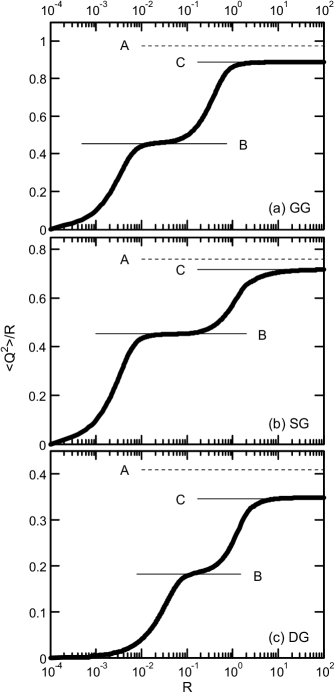
Figure 3: $\left\langle Q^{2}\right\rangle/R$ vs. $R$ for composite sources in which both the $a$ and $b$ beams have short range correlations.  The thick curves are the exact result in Eq. (1).  The solid lines labeled B are the theory in Eqs. (20)- (23), the dashed lines labeled A are the theory in Eqs. (24)- (27), whereas the solid lines labeled C are the short range screening result, Eq. (3).  (a) GG, beams $a$ and $b$ are Gaussians.  Beam parameters are $a=1,b=100,K=0.01$.  (b) SG, beam $a$ is a Sinc, beam $b$ is a Gaussian.  Beam parameters are the same as in (a).   (c) DG, beam $a$ is a Disk, beam $b$ is a Gaussian.  Beam parameters are $a=1,b=10,K=0.04$.  In all three examples displayed here the $b$ field was chosen to be a Gaussian in order to emphasize that the agreement with the theory represented by line B does not depend on the nature of the $a$ beam.  Other short range choices for the $b$ beam, Disk or Sinc, show equally good agreement.

We illustrate the above in Fig. 3 .  As can be seen, Eqs. (21)-(23) are good approximations to the exact results, whereas Eqs. (24)-(27) are good only to order of $10\%$.

We note that the well defined steps in this figure provide striking visual confirmation of the fact that there are two widely different length scales.  The first step starts, as expected, at $R\sim 1/b$, the second at $R\sim 1/a$.

VI BEAM $a$ EXHIBITS LONG-RANGE SCREENING, BEAM $b$ EXHIBITS SHORT-RANGE SCREENING

As discussed in the previous section, in region II, $1/b<R<1/a$, $\left\langle Q^{2}\right\rangle$ is dominated by $\left\langle Q^{2}\right\rangle_{b}$, Eqs. (21)- (23).  In region III, where $R>1/a$, beam $a$ exhibits long-range screening, and $\left\langle Q^{2}\right\rangle_{a}$ is given by Eq. (4) with $p=a$.  Neglecting again cross screening of $a$ and $b$ charges, the total charge variance in region III is approximated by the sum of $a$ and $b$ beam contributions, Eq. (24).

In Fig. 4 we plot $\left\langle Q^{2}\right\rangle/R$ vs. $R$ for RG and DG, again obtaining in the region of short range screening, region B, a plateau that is in good agreement with the calculated value for $\left\langle Q^{2}\right\rangle_{b}$.  As expected, in region A, the region of long range screening, $\left\langle Q^{2}\right\rangle/R$ grows linearly with $\ln R$.  We note that here not only is the calculated slope, Eq. (4), in close agreement with the exact result (thick curves), but also that Eq. (24) provides a rather reasonable description of the data.  Similar good agreement is obtained for RS (not shown).

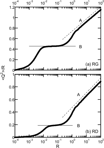
Figure 4: $\left\langle Q^{2}\right\rangle/R$ vs. $R$ for composite sources in which the $a$ beam has long-range and the $b$ beam short-range correlations.  The thick curves are the exact result in Eq. (1).  The solid lines labeled B are the short-range screening theory in Eqs. (20)- (22), the dashed lines labeled A are the long-range screening result in Eq. (4).  (a) RG, beam $a$ is a Ring, $b$ a Gaussian.  (b) RD, beam $a$ is a Ring, beam $b$ a Disk.  Beam parameters in both (a) and (b) are $\ a=1,b=100,K=0.01$.

VII BEAM $a$ EXHIBITS SHORT-RANGE SCREENING, BEAM $b$ EXHIBITS LONG-RANGE SCREENING

In region II, $1/b<R<1/a$, we again set $a=0$ in $W^{\left(\text{T}_{a}\text{T}_{b}\right)}$, and obtain for beam $b$ a Ring,

$$\left\langle Q^{2}\right\rangle_{b}\approx\frac{Kb^{2}}{4\pi}\int_{0}^{2R}\sqrt{4R^{2}-r^{2}}\frac{J_{1}^{2}\left(br\right)}{1-J_{0}\left(br\right)}dr.$$ (28)

As before, we have assumed $K\ll 1$, $\left[KW_{b}^{\left(\text{T}\right)}\right]^{2}\ll W_{b}^{\left(\text{T}\right)}$.  Proceeding as in [$19$, (Eqs. 40-48)], we obtain

$$\left\langle Q^{2}\right\rangle_{b} \approx\dfrac{KbR}{2\pi^{2}}\left[{\cal{F}}+\ln(bR)\right],$$ (29a)

$${\cal{F}} =\pi{\cal{I}}+\gamma+5\ln 2-3\approx 4.84258,$$ (29b)

$${\cal{I}} =\int_{0}^{\infty}\frac{J_{0}\left(x\right)J_{1}^{2}\left(x\right)}{1-J_{0}\left(x\right)}dx\approx 1.20946.$$ (29c)

We illustrate the above in Fig. 5.  In region B, $10^{-2}<R<10^{-1}$, for small $K$ ($0.015$) Eqs. (29) provide a good description of the exact result, Fig. 5(a), whereas when $K$ is no longer small ($0.2$) the expected deviations appear, Fig. 5(b).

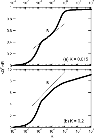
Figure 5: $\left\langle Q^{2}\right\rangle/R$ vs. $R$ for composite sources in which beam $a$ is a Gaussian with short-range correlations, and beam $b$ a Ring with long-range correlations.  Beam parameters are $\ a=1,b=100$.  The thick curves are the exact result in Eq. (1).  The solid lines labeled B are the long-range screening theory in Eqs. (29).  (a) $K=0.015$.  (b) $K=0.2.$

In Fig. 5(a) a plateau appears for $R>1$, apparently consistent with the fact that short-range screening $a$ field charges become important in this region.  But this apparent plateau is misleading, because the long-range screening of the $b$ field charges can never saturate: regardless of the nature of the $a$ field, $\left\langle Q^{2}\right\rangle/R$ for the $b$ charges must diverge logarithmically for large $R$.  The rate (slope) of this logarithmic divergence, however, is $K$ dependent, being small, Fig. 5(a) (large, Fig. 5(b)) for small (large) $K$.

VIII BOTH BEAM $a$ AND BEAM $b$ EXHIBIT LONG-RANGE SCREENING

The case of two Rings is illustrated in Fig. 6.  As before, Eq. (29) holds for the $b$ field charges.  But now the $a$ field charges also exhibit long-range screening, and $\left\langle Q^{2}\right\rangle/R$ exhibits the expected large $R$ logarithmic divergence also for small $K$ ($0.015$).

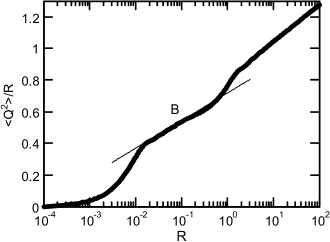
Figure 6: $\left\langle Q^{2}\right\rangle/R$ vs. $R$ for a composite source in which both beam $a$ and beam $b$ are Rings.  Beam parameters are $\ a=1,b=100$, $K=0.015$.  The thick curve is the exact result in Eq. (1).  The solid line labeled B is the long-range screening theory in Eqs. (29).

IX SUMMARY

Screening in speckled speckle produced by composite sources has been studied in the limit of two widely different characteristic length scales in the speckle pattern and two widely different intensities in the sources.  The interesting combination, emphasized here, is an intense field with a long length scale (the $a$ field) perturbed by a weak field that has a short length scale (the $b$ field).

Exact, and approximate, results have been presented for all four combinations of short- and long-range screening.  When the correlations in both fields are short-range, cross screening between $a$ and $b$ field singularities appears to be of only secondary importance, and the results of the exact calculation are found to decompose, approximately, into a sum of screening contributions, one for each field, Fig. 3.  A similar decomposition is found to hold if the $b$ field exhibits short-range screening and the $a$ field exhibits long-range screening, Fig. 4.  If the $b$ field exhibits long-range screening, however, then no decomposition is valid, Figs. 5 and 6.

The unusual screening properties of speckled speckle are most pronounced when the ratio ($b$ field to $a$ field) of length scales is $100:1$ or greater, and the ratio of optical powers in the sources (the parameter $K$) is $1:100$ or less.  Less extreme parameter ratios can also yield useful results, however, as in Fig. 3(b), so that the experimental study of screening in speckled speckle appears to be entirely feasible.

References

[1] J. F. Nye and M. V. Berry, “Dislocations in wave trains,” Proc. Roy. Soc. London Ser. A 336, 2165 (1974). For additional sources see online citation databases for the numerous papers that reference this work.

[2] J. F. Nye, Natural Focusing and the Fine Structure of Light (IOP Publ., London, 1999).

[3] J. W. Goodman, Speckle Phenomena In Optics (Roberts & Co., Englewood, Colorado, 2007).

[4] B. I. Halperin, “Statistical mechanics of topological defects,” in Physics of Defects, R. Balian, M. Kleman, and J.-P. Poirier, eds. (North-Holland, Amsterdam, 1981), p. 814-857.

[5] F. Liu and G. F. Mazenko, “Defect-defect correlation in the dynamics of first-order phase transitions,” Phys. Rev. B 46, 5963-5971 (1992).

[6] B. W. Roberts, E, Bodenschatz, and J. P. Sethna, “A bound on the decay of defect-defect correlation functions in two- dimensional complex order parameter equations,” Physica D 99, 252-268 (1996).

[7] I. Freund and M. Wilkinson, “Critical-point screening in random wave fields,” J. Opt. Soc. Am. A 15, 2892-2902 (1998).

[8] M. V. Berry and M. R. Dennis, “Phase singularities in isotropic random waves,” Proc. Roy. Soc. London A 456, 2059-2079 (2000); ibid., p. 3048.

[9] M. V. Berry and M. R. Dennis, “Polarization singularities in isotropic random vector waves,” Proc. Roy. Soc. Lond. A 457, 141-155 (2001).

[10] M. R. Dennis, “Polarization singularities in paraxial vector fields: morphology and statistics,” Opt. Commun. 213, 201-221 (2002).

[11] I. Freund, M. S. Soskin, and A. I. Mokhun, “Elliptic critical points in paraxial fields,” Opt. Commun. 208, 223-253 (2002).

[12] G. Foltin, “Signed zeros of Gaussian vector fields - density, correlation functions, and curvature,” J. Phys. A: Math. Gen. 36, 1729-1742 (2003).

[13] M. R. Dennis, “Correlations and screening of topological charges in Gaussian random fields,” J. Phys. A: Math. Gen. 36, 6611-6628 (2003).

[14] M. Wilkinson, “Screening of charged singularities of random fields,” J. Phys. A: Math. Gen. 37, 6763-6771 (2004).

[15] G. Foltin, S. Gnutzmann, and U. Smilansky, “The morphology of nodal lines - random waves versus percolation,” J. Phys. A: Math. Gen. 37, 11363-11372 (2004).

[16] B. A. van Tiggelen, D. Anache, and A. Ghysels, “Role of mean free path in spatial phase correlation and nodal screening,” Europhys. Lett. 74, 999-1005 (2006).

[17] I. Freund, R. I. Egorov, and M. S. Soskin, “Umbilic point screening in random optical fields,” Opt. Lett. 22, 2182-2184 (2007).

[18] R. I. Egorov, M. S. Soskin, D. A. Kessler, and I. Freund, “Experimental measurements of topological singularity screening in random paraxial scalar and vector optical fields,” Phys. Rev. Lett. 100, 103901 (2008).

[19] D. A. Kessler and I. Freund, “Short- and long-range screening of optical phase singularities and C points,” Opt. Commun. (2008), doi:10:1016/j.optcom.2008.05.018.

[20] I. Freund and D. A. Kessler, “Singularities in speckled speckle,” Opt. Lett. 33, 479-481 (2008).

[21] I. Freund and D. A. Kessler, “Singularities in speckled speckle: Statistics,” arXive:0806365; Opt. Commun. (submitted).

[22] J. W. Goodman, Statistical Optics (John Wiley, New York, 1985).

[23] M. Berry, “Disruption of wave-fronts: statistics of dislocations in incoherent Gaussian random waves,” J. Phys. A 11, 27-37 (1978).