Optimal quantum estimation in spin systems at criticality

Abstract

It is a general fact that the coupling constant of an interacting many-body Hamiltonian do not correspond to any observable and one has to infer its value by an indirect measurement. For this purpose, quantum systems at criticality can be considered as a resource to improve the ultimate quantum limits to precision of the estimation procedure. In this paper, we consider the one-dimensional quantum Ising model as a paradigmatic example of many-body system exhibiting criticality, and derive the optimal quantum estimator of the coupling constant varying size and temperature. We find the optimal external field, which maximizes the quantum Fisher information of the coupling constant, both for few spins and in the thermodynamic limit, and show that at the critical point a precision improvement of order $L$ is achieved. We also show that the measurement of the total magnetization provides optimal estimation for couplings larger than a threshold value, which itself decreases with temperature.

I Introduction

Acquiring information about a physical system involves observations and measurements, whose results are subjected to fluctuations, and one would like to eliminate or at least to minimize the corresponding errors. However, the precision of any measurement procedure is bounded by fundamental law of statistics and quantum mechanics, and in order to optimally estimate the value of some parameter, one has to exploit the tools provided by quantum estimation theory (QET) Helstrom .

As a matter of fact, many quantities of interest do not correspond to quantum observables. Relevant examples are given by the entanglement or the purity of a quantum state mg or the coupling constant of an interacting Hamiltonian. In these situations one needs to infer the value of the parameter through indirect measurements. For many-body quantum systems, changing the coupling constant drives the system into different phases and, in turn, this may be used to estimate the coupling itself. In particular, close to critical points, quantum states belonging to different phases should be distinguished more effectively than states belonging to the same phase pzPRE06 ; HQZ ; mcpg ; mcri ; lcvPRL07 ; pzpgmcPRL07 ; pzPRA07 . Distinguishability is usually quantified by fidelity between quantum states, i.e. overlap between ground state wave functions. In turn, the fidelity approach to quantum phase transitions (QPT) has recently attracted much attention pzPRE06 ; ZZL since, differently from bipartite entanglement measure approach letteraturaSpinChains , it considers the system as a whole, without resorting to bipartitions. In estimating the value of a parameter, one is led to define the Fisher information which represents an infinitesimal distance among probability distributions, and gives the ultimate precision attainable by an estimator via the Cramer-Rao theorem. Its quantum counterpart, the quantum Fisher information (QFI), is related to the degree of statistical distinguishability of a quantum state from its neighbors and, in fact, it turns out to be proportional to Bures metric between quantum states bur69 ; uhl76 ; woo81 ; jos94 ; QCR ; QCR2 ; bro9X ; nag00 .

As noticed in pzmp one can exploit the geometrical theory of quantum estimation to derive the ultimate quantum bounds to the precision of any estimation procedure, and the fidelity approach to QPTs to find working regimes achieving those bounds. Indeed, precision may be largely enhanced at the critical points in comparison to the regular ones. Here we show that the general idea advocated in pzmp can be successfully implemented in systems of interest for quantum information processing. To this aim we address a paradigmatic example of many-body system exhibiting a (zero temperature) QPT: the one-dimensional Ising model with a transverse magnetic field.

In most physical situations, some parameters of the Hamiltonian, e.g. the coupling constant, are unaccessible, whereas others may be tuned with reasonable control by the experimenter (e.g. external field). Therefore, the idea is to tune the controllable parameters in order to maximize the QFI and thus the distinguishability and the estimation precision. In doing this we consider the system both at zero and finite temperature, and fully exploit QET to derive the optimal quantum measurement for the unobservable coupling constant in terms of the symmetric logarithmic derivative. In the thermodynamic limit we find that optimal estimation is achieved tuning the field at the critical value, in accordance with pzmp , whereas at finite size $L$, the request of maximum QFI defines a pseudo-critical point which scales to the proper critical point as $L$ goes to infinity. In turn, a precision improvement of order $L$ may be achieved with respect to the non critical case.

The optimal measurement arising from the present QET approach may be not achievable with current technology. Therefore, having in mind a practical implementation, we consider estimators based on feasible detection schemes, and show, for systems of few spins, that the measurement of the total magnetization allows for estimation of the coupling constant with precision at the ultimate quantum level.

The paper is structured as follows: In Section II we briefly review some concepts of QET, introduce the symmetric logarithmic derivative and illustrate the quantum Cramer-Rao bound. We also review the notion of distance for the quantum Ising model. In Section III we derive the ultimate quantum limits to the precision of coupling constant estimation at zero temperature, both for the case of few spins and then in the thermodynamical limit. In Section IV we analyze the effects of temperature and derive the scaling properties of QFI. In Section V we address the measurement of total magnetization as estimator of the Hamiltonian parameter and show its optimality. Section VI closes the paper with some concluding remarks.

II Preliminaries

In this section we recall the basic concepts of QET and the metric approach to quantum criticality, specializing them to the one-dimensional Ising model in transverse field.

II.1 Quantum Estimation Theory

An estimation problem consists in inferring the value of a parameter $\lambda$ by measuring a related quantity $X$. The solution of the problem amounts to find an estimator $\hat{\lambda}\equiv\hat{\lambda}(x_{1},x_{2},\ldots)$, i.e. a real function of the measurements outcomes $\{x_{k}\}$ to the parameters space. Classically, the variance $\hbox{Var}(\lambda)=E[\hat{\lambda}^{2}]-E[\hat{\lambda}]^{2}$ of any unbiased estimator satisfies the Cramer-Rao theorem

$$\hbox{Var}(\lambda)\geq\frac{1}{MF(\lambda)}\>,$$

which establishes a lower bound on variance in terms of the number of independent measurements $M$ and the Fisher Information (FI) $F(\lambda)=E\left[\left(\partial_{\lambda}\log p(x|\lambda)\right)^{2}\right]$ i.e.

$$F(\lambda)=\sum_{x}p(x|\lambda)\left[\partial_{\lambda}\log p(x|\lambda)\right]^{2}\>,$$ (1)

$p(x|\lambda)$ being the conditional probability of obtaining the value $x$ when the parameter has the value $\lambda$. When quantum systems are involved $p(x|\lambda)=\hbox{Tr}\left[\varrho_{\lambda}\,P_{x}\right]$, $\{P_{x}\}$ being the probability operator-valued measure (POVM) describing the measurement. A quantum estimation problem thus corresponds to a quantum statistical model, i.e. a set of quantum states $\rho_{\lambda}$ labeled by the parameter of interest, with the mapping $\lambda\to\rho_{\lambda}$ providing a coordinate system. Upon introducing the Symmetric Logarithmic Derivative (SLD) $\Lambda_{\lambda}$ as the set of operators satisfying the equation

$$\partial_{\lambda}\rho_{\lambda}=\frac{1}{2}\Big{[}\Lambda_{\lambda}\rho_{\lambda}+\rho_{\lambda}\Lambda_{\lambda}\Big{]},$$ (2)

we can rewrite the FI as

$$F(\lambda)=\sum_{x}\frac{\mathop{\text{Re}}\nolimits\left(\textrm{Tr}\,\!\left[\rho_{\lambda}\Lambda_{\lambda}P_{x}\right]\right)^{2}}{\textrm{Tr}\,\!\left[\rho_{\lambda}P_{x}\right]}\>.$$ (3)

Then one can prove QCR ; QCR2 that $F(\lambda)$ is upper bounded by the Quantum Fisher Information

$$F(\lambda)\leq G(\lambda)\equiv\textrm{Tr}\,\!\left[\rho_{\lambda}\Lambda_{\lambda}^{2}\right]\>.$$ (4)

In turn, the ultimate limit to precision is given by the quantum Cramer-Rao theorem (QCR)

$$\hbox{Var}(\lambda)\geq\frac{1}{MG(\lambda)}\>,$$

which provides a measurement-independent lower bound for the variance which is attainable upon measuring a POVM built with the eigenprojectors of the SLD.

In the following we will consider the quantum statistical model defined by the set of Gibbs thermal states $\rho_{\lambda}=Z^{-1}e^{-\beta H(\lambda)}$, ($Z=\textrm{Tr}\,\![e^{-\beta H(\lambda)}]$) associated with a family $H(\lambda)$ of many-body Hamiltonians where $\lambda$ is the coupling constant we wish to estimate. The relevant observation at this point is that the Bures distance $d^{2}_{B}(\rho,\rho^{\prime})$ between quantum states at nearby points in parameter space may be written as

$$ds^{2}_{\lambda}\equiv d^{2}_{B}(\rho_{\lambda},\rho_{\lambda+d\lambda})=g_{\lambda}d\lambda^{2}=\frac{1}{4}G(\lambda)d\lambda^{2}$$ (5)

where $G(\lambda)$ is the QFI defined in Eq. (4) and $g_{\lambda}$ is Bures metric tensor given by SZ2003

$$g_{\lambda}=\frac{1}{2}\sum_{nm}\frac{\left|\langle\psi_{m}|\partial_{\lambda}\varrho_{\lambda}|\psi_{n}\rangle\right|^{2}}{p_{n}+p_{m}}\>,$$ (6)

$|\psi_{n}\rangle$ being the eigenvectors of $\rho_{\lambda}=\sum_{n}p_{n}|\psi_{n}\rangle\langle\psi_{n}|$. In other words, maxima of the Bures metric, e.g. the divergence occurring at QPTs pzpgmcPRL07 , correspond to optimal estimation working regimes. In the following we will systematically seek for maxima of Bures metric (QFI). In the thermodynamic limit those occur at the critical points pzpgmcPRL07 , whereas at finite size the maxima of the QFI define pseudo-critical points which scale to the actual critical points as the size goes to infinity.

II.2 Quantum Ising model

We are interested in systems which undergo a zero-temperature quantum phase transition and consider a paradigmatic example, the one-dimensional quantum Ising model of size $L$ with transverse field. The model is defined by the Hamiltonian

$$H=-J\sum_{k=1}^{L}\sigma_{k}^{x}\sigma_{k+1}^{x}-h\sum_{k=1}^{L}\sigma_{k}^{z},$$ (7)

where the $\sigma^{\alpha}_{i}$, are Pauli operators and we assume periodic boundary conditions $\sigma_{L+1}^{x}=\sigma_{1}^{x}$ unless stated otherwise. As the temperature and the field $h$ are varied one may identify different physical regions. At zero temperature, the system undergoes a QPT for $h=J$. For $h<J$ the system is in an ordered phase whereas for $h>J$ the field dominates, and the system is in a paramagnetic state. For temperature $T\ll\Delta$, $\Delta=\left|J-h\right|$ the system behaves quasi-classically, whereas for $T\gg\Delta$ quantum effects dominate. The Hamiltonian (7) can be exactly diagonalized by a Bogoliubov transformation, leading to

$$H=\sum_{k>0}\Lambda_{k}\left(\eta_{k}^{\dagger}\eta_{k}-1\right)\,,$$ (8)

where $\Lambda_{k}$ denotes the one particle energies and $\eta_{k}$ the fermion annihilation operator, $\Lambda_{k}=\sqrt{\epsilon_{k}^{2}+\Delta_{k}^{2}}$, $\Delta_{k}=J\sin(k)$, $\epsilon_{k}=(J\cos(k)+h)$. Strictly speaking, Eq. (8) holds in the sector with even number of fermions. In this case, periodic boundary conditions on the spins induce antiperiodic BC’s on the fermions and the momenta satisfy $k=\frac{(2n+1)\pi}{L}$. In the sector with odd number of particles, instead, one has $k=\frac{(2n)\pi}{L}$ and one must carefully treat excitations at $k=0$ and $k=\pi$. In any case, the ground state of (7) belongs to the even sector so that, at zero temperature we can use Eq. (8) for any finite $L$. At positive temperature we will be primarily interested in large system sizes and therefore we can neglect boundary terms in the Hamiltonian and use Eq. (8) in the whole Fock space. For small $L$ we will diagonalize explicitly the Hamiltonian (7), without resorting to (8).

The QFI for the parameter $J$ may be evaluated starting from Eq. (6) arriving at

$$G_{J}=\sum_{n}\frac{(\partial_{J}p_{n})^{2}}{p_{n}}+2\sum_{n\neq m}\left|\langle\psi_{n}|\partial_{J}\psi_{m}\rangle\right|^{2}\frac{(p_{n}-p_{m})^{2}}{p_{n}+p_{m}},$$ (9)

which, given $E_{j}=\sum_{k}n_{k}\Lambda_{k}$, where the $n_{k}$’s are the fermion occupation numbers, may be written as pzPRA07

$$G_{J}(J,h,\beta) = \frac{\beta^{2}}{4}\sum_{k}\frac{\left(\partial_{J}\Lambda_{k}\right)^{2}}{\cosh^{2}\left(\beta\Lambda_{k}/2\right)}$$ (10)

$$+ \sum_{k}\frac{\cosh\left(\beta\Lambda_{k}\right)-1}{\cosh\left(\beta\Lambda_{k}\right)}\left(\partial_{J}\vartheta_{k}\right)^{2}.$$

where $\vartheta_{k}=\hbox{arctan}\frac{\epsilon_{k}}{\Delta_{k}}$. Since the QFI is proportional to the Bures metric one may exploit the results derived for the Bures metric, which we recall here:

• At zero temperature, in the off-critical region (the thermodynamic limit) $L\gg\xi$, where $\xi$ is the system correlation length, the Bures metric behaves as $g_{\lambda}\sim L\left|\lambda-\lambda_{c}\right|^{-\Delta_{g}}$ close to the critical point. Here $L$ is the size of the system and $\Delta_{g}$ is related to the critical exponents of the transition, which turns out to be one for our system lcvPRL07 ; pzpgmcPRL07 .

• In the quasi-critical region $\xi\gg L$, $g_{\lambda}$ scales as $g_{\lambda}\sim L^{\alpha}$ with $\alpha=1+\Delta_{g}/\nu$ where $\nu$ is the correlation length critical exponent i.e. $\xi\sim|\lambda-\lambda_{c}|^{-\nu}$. It turns out that $\alpha=2$ quasi-free fermionic models, as the one considered here.

• At regular points (i.e. not-critical) the Bures metric is extensive i.e. $g_{\lambda}\sim L$.

• As the temperature is turned on, as long as it is small but larger than the energy gap of the system, quantum-critical effects dominate. In this region $T\gg\Delta$, thermodynamic quantities scales algebraically with the temperature and one has $g_{\lambda}\sim T^{-\beta}$, with $\beta>0$. For the Ising model $\beta=1$ pzPRA07 .

In the following, we will exploit the dramatic increase of the QFI that one experiences in the critical regions, to improve the ultimate quantum limit achievable in the estimation of the coupling parameter.

III QET at zero temperature

In this section we begin to test the idea of estimating the coupling constant $J$ of the Ising model by finding the maximum of QFI at zero temperature, where the system is in the ground state. At first we consider systems made of few spins and then we address the thermodynamic limit.

III.1 Small $L$

We start with the case of $L=2,3$ and $4$ in Eq.(7). The QFI is obtained from Eq.  (9) by explicit diagonalization of the Ising Hamiltonian where $p_{n}=e^{-\beta E_{n}}/Z$, $E_{n}$ and $|\psi_{n}\rangle$ are the eigenvalues and eigenvectors of $H$. For example, for $L=2$ we have $E_{n}=\pm 2J,\pm 2\sqrt{J^{2}+h^{2}}$ and $Z=2\cosh(2\beta J)+2\cosh(2\beta\sqrt{J^{2}+h^{2}})$. For $T=0$ one gets

$$G_{J}(J,h,0) = \frac{h^{2}}{(h^{2}+J^{2})^{2}},\quad L=2$$

$$G_{J}(J,h,0) = \frac{3h^{2}}{4(h^{2}-hJ+J^{2})^{2}},\quad L=3$$

$$G_{J}(J,h,0) = \frac{h^{2}(h^{4}+4h^{2}J^{2}+J^{4})}{(h^{4}+J^{4})^{2}},\quad L=4\,.$$ (11)

Maxima of $G_{J}$ are obtained for $h^{\ast}=J$ for $L=2,3,4$. Actually, this is true for any $L$, see also the next Section, and the pseudo-critical point $h^{\ast}$ which maximizes $G_{J}$, turns out to be independent of $L$ and equal to the true critical point, $h_{c}=J,\,\forall L$. At its maximum $G_{J}$ goes like $1/J^{2}$ and the ultimate lower bound to precision (variance) of any quantum estimator of $J$ scales as $J^{2}$.

III.2 Large $L$

In the following we discuss the QFI for a system of size $L$. We analyze the behavior of $G_{J}$ near the critical region at $T=0$. Taking the limit $T\to 0$ in Eq.(10), the classical elements of the Bures metric, which depends only on thermal fluctuations, vanishes due to the factor of $(\cosh(\beta\Lambda_{k}/2))^{-2}$. Therefore, at zero temperature, only the nonclassical part of Eq.(10) survives and one obtains

$$G_{J}=\sum_{k}(\partial_{J}\vartheta_{k})^{2},$$ (12)

where $\partial_{J}\vartheta_{k}=\frac{1}{1+(\Delta_{k}/\epsilon_{k})^{2}}(\partial_{J}\frac{\Delta_{k}}{\epsilon_{k}})=\frac{-h\sin k}{\Lambda_{k}^{2}}$. Since we are in the ground state, the allowed quasi-momenta are $k=\frac{(2n+1)\pi}{L}$ with $n=0,\ldots,L/2-1$. Explicitly we have

$$G_{J} = \sum_{k}\frac{h^{2}\sin(k)^{2}}{\Lambda_{k}^{4}}.$$ (13)

We are interested in the behavior of the QFI in the quasi-critical region $\xi\gg L$. In the Ising model $\nu=1$ so the critical region is described by small values of the scaling variable $z\equiv L(h-J)\simeq L/\xi$, that is $z\approx 0$. Conversely the off-critical region is given by $z\rightarrow\infty$. We substitute $h=J+z/L$ in Eq.(13) and expand around $z=0$ to obtain the scaling of $G_{J}$ in the quasi-critical regime

$$G_{J}=\sum_{k_{n}}\frac{(J+\frac{z}{L})^{2}\sin^{2}(k_{n})}{[\frac{z^{2}}{L^{2}}+4J(J+\frac{z}{L})\sin^{2}(k_{n}/2)]^{2}}\equiv\sum_{k_{n}}f_{k_{n}}(z)\,.$$ (14)

Since $\partial_{z}f(0)=0$, the maximum of $G_{J}$ is always at $z=0$ for all values of $L$, in turn, the pseudo-critical point is $h_{L}^{\ast}=J=h_{c}$ $\forall L$. As already noticed previously, the statement $h_{L}^{\ast}=h_{c}$ is peculiar to this particular situation. For instance, introducing an anisotropy $\gamma$ so as to turn the Ising model into the anisotropic $XY$ model, the pseudo-critical point gets shifted and one recovers the general situation $h_{L}^{\ast}=h_{c}+O\left(L^{-\theta}\right)$. Going to second order one obtains

$$\sum_{k}(\partial_{J}\theta_{k})^{2} = \sum_{k_{n}}\frac{1}{4J^{2}}\cot^{2}(k_{n}/2)\Big{(}1-\frac{z^{2}}{2J^{2}L^{2}}\times$$ (15)

$$\frac{1}{\sin^{2}(k_{n}/2)}\Big{)}+O\left(z^{3}\right)\,.$$

Using Euler-Maclaurin formula EMC we get

$$G_{J}=L^{2}\left(\frac{1}{8J^{2}}-\frac{z^{2}}{384J^{4}}\right)-\frac{L}{8J^{2}}+O(L^{0}).$$ (16)

This shows explicitly that at $h=J$ the Fisher information has a maximum and there it behaves as

$$G_{J}(L,T=0,h^{\ast}=J)\simeq\frac{L^{2}}{8J^{2}}+O(L).$$ (17)

We observe that superextensive behavior of the QFI in the quasi-critical region around the QPT, $G_{J}\sim L^{2}$, implies that the estimation accuracy scales like $L^{-2}$ at the critical points, while it goes like $L^{-1}$ at regular points.

III.3 Signal-to-noise ratio

Notice that, in assessing the estimability of a parameter $\lambda$, the quantity to be considered is the quantum signal-to-noise ratio (QSNR) given by $Q(\lambda)\equiv\lambda^{2}G(\lambda)$ which takes into account of the scaling of the variance and the mean value of a parameter rather than its absolute value. We say that a parameter $\lambda$ is effectively estimable when the corresponding $Q(\lambda)$ is large and that to a diverging QFI corresponds the optimal estimability. In both cases of few and many spins, at the critical point the QFI goes like $1/J^{2}$, this means that $Q(J)$ is independent on $J$ and one can estimate large as well as small values of parameters without loss of precision.

IV QET at finite temperature

In this section we consider the estimation the coupling constant $J$ at finite temperature. We first discuss in some detail the short chains with $L=2,3,4$ and then we treat the case $L\gg 1$.

IV.1 Small $L$

As a warm-up let us first focus on the simplest, $L=2$ case. A first step in the computation of the SLD for two qubit is to find the SLD in the single qubit case. Consider a system with ”Hamiltonian” $H=\mathbf{a}\cdot\mbox{\boldmath$\sigma$}$ in the state $\rho=e^{-\mathbf{a}\cdot\mbox{\scriptsize\boldmath$\sigma$}}Z^{-1}$ where $Z=\mathrm{Tr}e^{-\mathbf{a}\cdot\mbox{\scriptsize\boldmath$\sigma$}}$, and the three-component vector $\mathbf{a}$ depends on parameter $J$. The SLD relative to this state turns out to be

$$\Lambda= -\tanh\left(a\right)\left(\partial_{J}\hat{\mathbf{a}}\cdot\mbox{\boldmath$\sigma$}\right)$$

$$-\left[1+\tanh\left(a\right)-2\tanh\left(a\right)^{2}\right]\left(\partial_{J}a\right)\left(\hat{\mathbf{a}}\cdot\mbox{\boldmath$\sigma$}\right)\,.$$ (18)

where $a$ is the modulus of $\mathbf{a}$ and $\hat{\mathbf{a}}=\mathbf{a}/a$. Now note that the Hamiltonian (7) for $L=2$ (with PBC), has the following block-diagonal form in the basis $\left\{|++\rangle,\,|--\rangle,\,|+-\rangle,\,|-+\rangle\right\}$:

$$H=-2\beta\left(\begin{array}[]{cc}J\sigma^{x}+h\sigma^{z}&0\\ 0&J\sigma^{x}\end{array}\right).$$ (19)

We can then apply formula (18) in each subspace to obtain the full SLD. After some algebra one realizes that the SLD has the following form

$$\Lambda=c_{1}\sigma^{x}\otimes\sigma^{x}+c_{2}\sigma^{y}\otimes\sigma^{y}+c_{3}\left(\sigma^{z}\otimes\leavevmode{\rm 1\mkern-4.8muI}+\leavevmode{\rm 1\mkern-4.8muI}\otimes\sigma^{z}\right),$$ (20)

where $c_{1,2,3}$ are constants which depend on $\beta,J$, and $h$. When the temperature is sent to zero the above expression becomes

$$\Lambda_{T=0}= \frac{h}{2\left(J^{2}+h^{2}\right)^{3/2}}\Big{[}h\left(\sigma^{x}\otimes\sigma^{x}-\sigma^{y}\otimes\sigma^{y}\right)$$

$$-J\left(\sigma^{z}\otimes\leavevmode{\rm 1\mkern-4.8muI}+\leavevmode{\rm 1\mkern-4.8muI}\otimes\sigma^{z}\right)\Big{]}.$$ (21)

We see that, already in the simple two-qubit case, the SLD is a complicated operator both at positive and at zero temperature. More involved expressions are obtained $L=3,4$ and larger. We do not report here the analytic expression of the corresponding QFIs $G_{J}$ for $L=2,3,4$ since they are a bit involved. Rather, in order to assess estimation precision at finite temperature and compare it to that at $T=0$, we consider the ratio $\gamma_{J}=G_{J}(\beta,J,h)/G_{J}(\infty,J,h)$, for some fixed values of $J$ and illustrate its behavior by means of few plots.

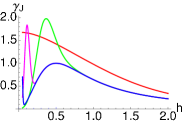
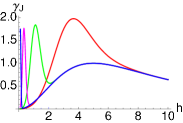
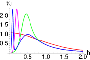
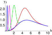
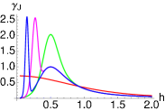
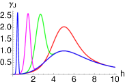
Figure 1: The ratio $\gamma_{J}$ as a function of $h$ for $L=2,3,4$ (from top to bottom) and $J=0.5$ (on the left), $J=5$ (on the right). The colors refer to different values of $\beta=1$ (red), $\beta=10$ (green), $\beta=100$ (purple), $\beta=1000$ (blue).

As it is apparent from Fig. 1 for small $h$ the ratio is smaller than $1$, i.e estimation of $J$ is more precise at zero temperature, whereas for increasing $h$ a finite temperature may be preferable. In turn, for any value of $J$ and $\beta$, there is a field value that makes finite temperature convenient: this is true also for low temperature as proved by the presence of a global maximum for small $h$, besides the local maximum at $h=J$. For $\beta\rightarrow\infty$ the maxima at small $h$ disappears and we recover the zero temperature results. Notice that, in view of Eqs. (11), the ratio $\gamma_{J}$ is proportional to the QSNR. Besides, since the maxima of $\gamma_{J}$ vary with $\beta$, we conclude that the optimal field $h^{\ast}$ which maximizes $G_{J}(\beta)$ varies with the temperature. This is illustrated for $L=2$ in Fig. 2, where we report the log-linear plot of $G_{J}(\beta)$ as a function of $h$ for different values of $J$ and $\beta$. For high temperature the maxima are localte at a field value close to zero, whereas for decreasing temperature they move towards $h^{\ast}=J$.

Figure 2: Logarithmic plot of $G_{J}(\beta)$ vs $h$ for (from top to bottom) $J=0.1$, $0.5$, $1$, $2$,$5$, $8$ and $\beta=1$ (left), $\beta=10$ (right).

IV.2 Large $L$

At positive temperature and $L$ large, the sums in equation (10) may be replaced by $L\int dk$. The quantity $\tilde{G}_{J}\equiv G_{J}/L$ is always convergent, and the convergence rate is exponentialy fast in $L$ in the (renormalized classical) region $T\ll\Delta$ whereas is effectively only algebraic when $T\gg\Delta$ (the quantum-critical region). Thus, up to contribution vanishing with $L$, $\tilde{G}_{J}=\tilde{G}_{J}^{1}+\tilde{G}_{J}^{2}$ is a bounded function of its arguments as long as $T>0$, given by

$$\tilde{G}_{J}^{1} = \frac{\beta^{2}}{8\pi}\int_{0}^{\pi}\frac{dk}{\cosh^{2}\left(\beta\Lambda_{k}/2\right)}\frac{\left(J+h\cos\left(k\right)\right)^{2}}{\Lambda_{k}^{2}}$$ (22)

$$\tilde{G}_{J}^{2} = \frac{1}{2\pi}\int_{0}^{\pi}dk\frac{\cosh\left(\beta\Lambda_{k}\right)-1}{\cosh\left(\beta\Lambda_{k}\right)}\frac{h^{2}\sin\left(k\right)^{2}}{\Lambda_{k}^{4}}\,.$$ (23)

For any $T>0$ the function $\tilde{G}_{J}$ has a cusp in $h=J$, where it achieves its maximum value. Changing variable from momentum to energy, the integrals above can be approximately evaluated in the quantum critical region $\beta\left|J-h\right|\ll 1$ (actually we also require low temperature, i.e. $\beta\left|J+h\right|\gg 1$). The result is

$$\tilde{G}_{J}^{1} = \frac{9\zeta\left(3\right)}{8\pi}\frac{T}{J^{2}\left|J+h\right|}+O\left(T^{0}\right)$$ (24)

$$\tilde{G}_{J}^{2} = \frac{\mathcal{C}}{\pi^{2}}\frac{\left|J+h\right|}{TJ^{2}}-\frac{1}{8J^{2}}+O\left(T\right)\,,$$ (25)

where $\mathcal{C}$ is Catalan’s constant $\mathcal{C}=0.915$ and the Riemann Zeta-function gives $\zeta(3)=1.202$.

In summary, for large sizes and at positive temperature, the maximum of the QFI as a function of $h$ is always located at $h=J$ for all values of $J,T$. At the maximum, the QFI is approximately given by

$$G_{J}\simeq\frac{2\mathcal{C}}{\pi^{2}}\frac{L}{TJ}.$$ (26)

As a consequence, the QSNR scales as $Q_{J}\sim JL/T$, in other words, at finite temperature, the estimation of small values of the coupling constant is unavoidably less precise than the estimation of large values. As expected, large $L$ and/or low temperature improve the precision of estimation.

V Practical implementations

The SLD represents an optimal measurement, i.e. the corresponding Fisher information is equal to the QFI. However, as we have seen [see e.g. Eq. (21)], generally the SLD does not correspond to an observable whose measurement can be easily implemented in practice. Therefore, in this section, we consider the total magnetization $M_{z}=\frac{1}{L}\sum_{i}\sigma^{z}_{i}$, as a feasible and natural measurement to be performed on the system in order to estimate the coupling $J$. We assume that the system is at thermal equilibrium, $\rho=Z^{-1}e^{-\beta H}$, and consider short chains $L=2,3,4$. We illustrate the procedure in detail for the simplest $L=2$ case. Upon measuring $M_{z}$, the possible outcomes are $m=\{1,0,-1\}$ with eigenprojectors $P_{m}$ given by $P_{1}=|00\rangle\!\langle 00|$, $P_{-1}=|11\rangle\!\langle 11|$, and $P_{0}=|10\rangle\!\langle 10|+|01\rangle\!\langle 01|$. The corresponding probabilities $p(m|J)=\textrm{Tr}\,\!(\rho P_{m})$ are given by

$$p(\pm 1|J)= \frac{\cosh(2\beta\sqrt{J^{2}+h^{2}})}{2\left[\cosh(2\beta J)+\cosh(2\beta\sqrt{J^{2}+h^{2}})\right]}\times$$ (27)

$$\Big{(}1\pm h(J^{2}+h^{2})^{-1/2}\tanh(2\beta\sqrt{J^{2}+h^{2}})\Big{)}$$

$$p(0|J)= \frac{\cosh(2\beta J)}{\cosh(2\beta J)+\cosh(2\beta\sqrt{J^{2}+h^{2}})}\,.$$ (28)

The FI is then obtained by substituting $p(m|J)$ into Eq. (1). The resulting expression provides a bound for the variance of any estimator of $J$ based on $M$ measurements of magnetization: $\hbox{Var}(J)\geq 1/MF_{J}$.

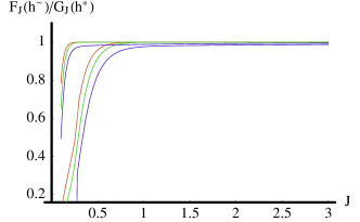
Figure 3: The ratio $F_{J}(\beta,J,h\hbox{\~{}})/G_{J}(\beta,J,h^{\ast})$ as a function of $J$ for $L=2$ (red line), $L=3$ (green line), and $L=4$ (blue line). The bottom group of lines is for $\beta=3$, whereas the top group is for $\beta=10$.

The Braunstein-Caves inequality says that the FI of any measurement $F_{J}$ is upper bounded by the QFI $G_{J}$. For the magnetization this is illustrated in Fig. 3, where we plot of the ratio $F_{J}(\beta,J,h\hbox{\~{}})/G_{J}(\beta,J,h^{\ast})$ for $L=2,3,4$, $h\hbox{\~{}}$ being the field maximizing the FI. Notice that for increasing $J$ the FI of the magnetization saturate to the QFI, i.e. magnetization measurement becomes optimal. The saturation is faster for lower temperature (we report the ratio for $\beta=3$ and $\beta=10$). Notice also that for low temperature the dependence of the ratio on the size $L$ almost disappears. In summary: for any temperature there is a threshold value for $J$, above which the measurement of the magnetization is optimal for the estimation of $J$ itself. This threshold value decreases with temperature, and for zero temperature magnetization is optimal for any $J$. Indeed, after explicit calculation of Eq. (1) for $L=2,3,4$ we found that, in the limit $T\to 0$, $F_{J}(h,T=0)=G_{J}(h,T=0)$, i.e.  the FI of the magnetization is equal to the QFI. In other words the estimation based on magnetization may achieve the ultimate bound to precision imposed by quantum mechanics. Besides, at finite temperature, despite the fact that the equality does not hold exactly, $F_{J}$ is only slightly grater than $G_{J}$ almost in the whole parameter range $(J,T)$. This may be also seen in the behavior of $F_{J}$ versus temperature: the ratio $\delta_{J}=F_{J}(\beta,J,h)/F_{J}(\infty,J,h)$ at fixed $J$ may be greater than $1$ for some values of the magnetic field, namely magnetization measurements may be more precise at finite $T$, as it happens for the optimal measurement with precision bounded by the QFI. Of course, for $T\rightarrow 0$, $\delta_{J}\to 1$.

Overall, we conclude that the magnetization $M_{z}$ is a good candidate for nearly optimal estimation. Of course we still need an efficient estimator, that is an estimator actually saturating the (classical) Cramer-Rao bound. To this aim we employ a Bayesian analysis, since Bayes estimators are known to be asymptotically efficient LeCam , i.e. $\hbox{Var}(J_{B})=1/MF_{J}$, for $M\gg 1$, $J_{B}$ being the Bayesian estimator (see below). According to the Bayes rule, given a set of outcomes $\{m\}$ from $M$ independent measurements of the magnetization, the a-posteriori distribution for the parameter $J$ is given by $p(J|\{m\})=1/N\prod_{m}p(m|J)^{n_{m}}$ where $N$ is a normalization constant and $n_{m}$ is the number of measurements with outcome $m$. Bayes estimator is the mean $J_{B}=\int dJ\>J\>p(J|\{m\})$ of the a-posteriori distribution and precision is quantified by the corresponding variance. In the asymptotic limit of many measurements $M\gg 1$, $n_{m}\to Mp(m|J^{\ast})$ where $J^{\ast}$ is the true value of the parameter to be estimated and the a posteriori distribution rewrites as $p_{a}(J|\{m\})=1/N\sum_{m}\exp\left[Mp(m|J^{\ast})\log p(m|J)\right]$. In order to check the actual meaning of ”asymptotic” we have performed a set of Monte Carlo simulated experiments of the whole measurement process. In Fig. 4, we report the result of Monte Carlo simulated experiments of magnetization measurements for $J=3$ and $\beta=1$. The black dots represent the mean variance of the Bayes estimator $J_{B}$ averaged on $20$ sets each of $500$ measurements. The blue line is the corresponding variance evaluated using the asymptotic a-posteriori distribution, whereas the green line is the Cramer-Rao bound $(MF_{J})^{-1}$. The plot shows that Bayes estimator is indeed asymptotically efficient and that already with a few hundreds of measurements one may achieve the ultimate precision. Overall, putting this result together with the fact $F_{J}\simeq G_{J}$ (see Fig. 3) we conclude that the measurement of the total magnetization of the system provides a nearly optimal and feasible measurement (at any $\beta$) to estimate the coupling of the one-dimensional quantum Ising model.

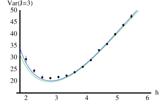
Figure 4: Estimation of the coupling constant by magnetization measurement and Bayesian analysis. The plot is for $L=2$ and $\beta=1$ with true value of the coupling equal to $J=3$. We report the variance of the Bayesian estimator for Monte Carlo simulated experiments (M=500, black dots), the corresponding variance evaluated using the asymptotic a-posteriori distribution (blue line), and the (classical) Cramer-Rao bound (green line).

VI Conclusions

The coupling constant of a many-body Hamiltonian is not an observable quantity and we have to solve a quantum statistical model to evaluate the bounds to its estimation precision. This has fundamental implications since it corresponds to find the ultimate limits imposed by quantum mechanics to the distinguishability of different states of matter. In this paper we exploited the equivalence between the quantum Fisher metric and the (ground or thermal) Bures metric and all the results recently obtained for the latter. Specifically at zero temperature, the Bures metric scales with the system size $L$ at regular points whereas it can increases as $L^{2}$ at or in the vicinity of quantum critical point. A similar enhancement takes place when temperature is considered. In turn it is possible to exploit this enhancement to dramatically improve the bounds to precision in a quantum estimation problem. Let us imagine that an experimenter would like to infer the value of a coupling constant of a physical system over which he has little or no control. Reasonably the experimenter has good control over the external fields he can apply to the system. The idea is then to tune the external field to a value close to the quantum critical point. At this value of the couplings, an improvement of order of $L$ can be achieved in the precision of the estimation of the unknown coupling. To test these ideas in practice, we have worked out in detail a specific example, the 1D quantum Ising model. This model provides us with all the ingredients we need, a coupling constant $J$, an external field $h$, and a quantum critical point at $h=J$. The main accomplishments of our analysis are: i) At zero temperature we evaluated the precision in the estimation of the coupling, exactly for short chains of $L=2,3,4$ sites and asymptotically for large $L$. We found that the optimal estimation is possible at values of the field exactly equal to the critical point, independently of $L$. For large $L$ we indeed observe a $1/L$ enhancement of precision, and a quantum signal-to-noise ratio independent of the coupling. ii) At positive temperature the optimal value of the field is again given by the critical value when the system size is large or the temperature is low. In the other working regimes the optimal field maximizing the quantum Fisher information, defines a set of pseudo-critical points, and the optimal precision scales as $TJ/L$. iii) We obtained the optimal observable for estimation in terms of the symmetric logarithmic derivative and showed that already in the case $L=2$ it does not correspond to an easily implementable measurement. iv) We have shown that for small $L$ the measurement of the total magnetization allows to achieve ultimate precision. Using Monte Carlo simulated experiments and Bayesian analysis we proved that this is possible already after a limited number of measurements of the order of few hundreds. We conjecture that this may be true for any $L$; work along this line in progress.

Overall, we found that criticality is a resource for precise characterization of interacting quantum systems (e.g. a quantum register), and may represent a relevant tool for the development of integrated quantum networks.

References

- (1) C. W. Helstrom, Quantum Detection and Estimation Theory (Academic Press, New York, 1976); A. S. Holevo, Statistical Structure of Quantum Theory, Lect. Not. Phys 61, (Springer, Berlin, 2001).
- (2) M. G. Genoni, P. Giorda, and M. G. A. Paris, arXiv:0804.1705 .
- (3) P. Zanardi and N. Paunković Phys. Rev. E 74, 031123 (2006)
- (4) H. Q. Zhou, arXiv: cond-mat/0701608; H. Q. Zhou et al., arXiv:0704.2940.
- (5) M. Cozzini, P. Giorda, and P. Zanardi, Phys. Rev. B 75, 014439 (2007).
- (6) M. Cozzini, R. Ionicioiu, and P. Zanardi, Phys. Rev. B 76, 104420 (2007).
- (7) L. Campos Venuti and P. Zanardi, Phys. Rev. Lett. 99, 095701 (2007).
- (8) P. Zanardi, P. Giorda, and M. Cozzini, Phys. Rev. Lett. 99, 100603 (2007).
- (9) P. Zanardi, L. Campos Venuti, and P. Giorda, Phys. Rev. A 76, 062318 (2007).
-
(10)
We have
- (11) H.-Q. Zhou and J. P. Barjaktarevic, e-prind arXiv:cond-mat/071608; H.-Q. Zhou, J.-H. Li, and B. Li, e-print arXiv:0704.2945.
- (12) T. J. Osborne, and M. A. Nielsen, Phys. Rev. A 66, 032110 (2002); A. Osterloh, L. Amico, G: Falci, and R. Fazio, Nature (London) 416, 608 (2002); G. Vidal, J. I. Latorre, E. Rico, and A. Kitaev, Phys. Rev. Lett. 90, 227902 (2003).
- (13) P. Zanardi and M. G. A. Paris, e-print arXiv:0708.1089
- (14) S. Braunstein and C. Caves, Phys. Rev. Lett. 72, 3439 (1994).
- (15) S. Braunstein, C. Caves, and G. Milburn, Ann. Phys. 247, 135 (1996).
- (16) D. Bures, Trans. Am. Math. Soc. 135, 199 (1969).
- (17) A. Uhlmann, Rep. Math. Phys. 9, 273 (1976).
- (18) R. Josza, J. Mod. Opt. 41, 2314 (1994).
- (19) W. K. Wootters Phys. Rev. D 23, 357 (1981).
- (20) D. C. Brody, L. P. Hughston, Proc. Roy. Soc. Lond. A 454, 2445 (1998); A 455, 1683 (1999).
- (21) A. Sun-Ichi, H. Nagaoka, Methods of information geometry (AMS, 2000).
- (22) H.-J. Sommers, K. Zyczkowski, J. Phys. A 36, 10083 (2003).
- (23) L. LeCam, Asymptotic Methods in Statistical Decision Theory (Springer-Verlag, New York, 1986).