Bayes-optimal inverse halftoning and statistical mechanics of the Q-Ising model

Abstract

On the basis of statistical mechanics of the Q-Ising model, we formulate the Bayesian inference to the problem of inverse halftoning, which is the inverse process of representing gray-scales in images by means of black and white dots. Using Monte Carlo simulations, we investigate statistical properties of the inverse process, especially, we reveal the condition of the Bayes-optimal solution for which the mean-square error takes its minimum. The numerical result is qualitatively confirmed by analysis of the infinite-range model. As demonstrations of our approach, we apply the method to retrieve a grayscale image, such as standard image Lenna, from the halftoned version. We find that the Bayes-optimal solution gives a fine restored grayscale image which is very close to the original.

1 Introduction

In recent two or three decades, a considerable number of researchers have investigated various problems in information sciences, such as image restoration and error-correcting codes on the basis of the analogy between statistical mechanics and probabilistic information processing [1]. Especially, a lot of researchers have investigated various problems in image processing based on the Markov random fields [2, 3, 4, 5]. In the field of the print technologies, many techniques of information processing have also developed. Particularly, the digital halftoning [7, 8, 9, 10, 11] is regarded as a key processing to convert a digital grayscale image to black and white dots which represents the original grayscale levels appropriately. On the other hand, the inverse process of the digital halftoning is referred to as inverse halftoning. The inverse halftoning is also important for us to make scanner machines to retrieve the original grayscale image by making use of much less informative materials, such as the halftoned binary dots. The inverse halftoning is ‘ill-posed’ in the sense that one lacks information to retrieve the original image because the material one can utilize is just only the halftoned black and white binary dots instead of the grayscale one. To overcome this difficulty, we usually introduce the ‘regularization term’ which compensates the lack of the information and regard the inverse problem as a combinatorial optimization [12, 13]. Then, the optimization is achieved to find the lowest energy state via, for example, simulated annealing [14, 15].

Besides the standard regularization theory, we can use the Bayesian approach. Under the direction of this approach, Stevenson [16] attempted to apply the maximum of a Posteriori (MAP for short) estimation to the problem of inverse halftoning for a given halftone binary dots obtained by the threshold mask and the so-called error diffusion methods. However, there is few theoretical approach to deal with the inverse-halftoning from the view point of the Bayesian inference and statistical mechanics of information.

In this study, on the basis of statistical mechanics of the Q-Ising model [17], we formulate the problem of inverse halftoning to estimate the original grayscale levels by using the information about both the halftoned binary dots and the threshold mask. We reconstruct the original grayscale revels from a given halftoned binary image and the threshold mask so as to maximize the posterior marginal probability. Using Monte Carlo simulations, we investigate statistical properties of the inverse process, especially, we reveal the condition of the Bayes-optimal solution for which the mean-square error takes its minimum. The result of the simulation is supported by the analysis of the infinite-range model. In order to investigate to what extent the Bayesian approach is effective for realistic images, we apply the method to retrieve the grayscale levels of the 256-levels standard image Lenna from the binary dots. We find that the Bayes-optimal solution gives a fine restored grayscale image which is very close to the original one.

The contents of this paper are organized as follows. In the next section, we formulate the problem of inverse halftoning. We mention the relationship between statistical mechanics of the Q-Ising model and Bayesian inference of the inverse halftoning. In the following section, we investigate statistical properties of the Bayesian inverse halftoning by Monte Carlo simulations. Analysis of the infinite-range model supports the result of the simulations. We also show that the Bayes-optimal inverse halftoning is useful even for realistic images, such as the 256-level standard image Lenna. Last section is summary.

2 The model

We first define the model system to investigate the statistical performance of the Bayesian inference for the problem of inverse halftoning. As original grayscale images, which are converted to the black and white binary dots, we consider snapshots from a Gibbs distribution of the ferromagnetic Q-Ising model having the spin variables $\{\xi\}\equiv\{\xi_{x,y}=0,\cdots,Q-1|x,y=0,\cdots,L-1\}$. Then, each image $\{\xi\}$ being specified by the Hamiltonian $H(\{\xi\})=J_{s}\sum_{n.n.}(\xi_{x,y}-\xi_{x^{{}^{\prime}},y^{{}^{\prime}}})^{2}$ follows the Gibbs distribution

$${\rm Pr}\left(\{\xi\}\right)=\frac{1}{Z_{s}}\exp\left[-\frac{H(\{\xi\})}{T_{s}}\right]=\frac{1}{Z_{s}}\exp\left[-\frac{J_{s}}{T_{s}}\sum_{\rm n.n.}\left(\xi_{x,y}-\xi_{x^{{}^{\prime}},y^{{}^{\prime}}}\right)^{2}\right]$$ (1)

at temperature $T_{s}$, where $Z_{s}$ is the partition function of the system and the summation $\sum_{\rm n.n.}(\cdots)$ runs over the sets of the nearest neighboring pixels located on the square lattice in two dimension. The ratio of strength of spin-pair interaction $J_{s}$ and temperature $T_{s}$, namely, $J_{s}/T_{s}$ controls the smoothness of our original image $\{\xi\}$. In Fig. 1 (left), we show a typical example of the snapshots from the distribution (1) for the case of $Q=4$, $J_{s}=1$ and $T_{s}=0.5$.

         

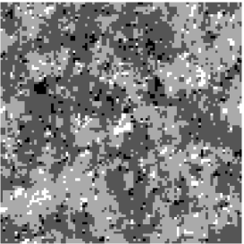
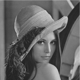
Figure 1: An original image as a snapshot from the Gibbs distribution of (1) having $100\times 100$ pixels for the case of $Q=4$ (left). We set $T_{s}=0.5$, $J=1$. The right panel shows a $256$-levels standard image Lenna with $400\times 400$ pixels.

The right panel of the Fig. 1 shows the 256-levels grayscale standard image Lenna with $400\times 400$ pixels. We shall use the standard image to check the efficiency of our approach in the last part of this paper.

In order to convert original grayscale images to the the black and white binary dots, we make use of the threshold array $\{M\}$.

0	2
3	1

                0 8 2 10 12 4 14 6 3 11 1 9 15 7 13 5

Figure 2: The Bayer-type threshold arrays for the dither method with $2\times 2$ (left) and with $4\times 4$ (right).

Each component $M_{k,l}$ of the array $\{M\}$ takes a non-overlapping integer and these numbers are arranged on the $L_{m}\times L_{m}$ squares as shown in Fig. 2 for $L_{m}=2$ (left) and for $L_{m}=4$ (right). For general case of $L_{m}$, we define the array as

$$\{M\} = \left\{M_{k,l}=0,\frac{Q-1}{L_{m}^{2}-1},\frac{2(Q-1)}{L_{m}^{2}-1},\cdots,Q-1{\biggr{|}}k,l=0,1,\cdots,L_{m}-1\right\}.$$

We should keep in mind that the definition (LABEL:eq:mask) is reduced to $\{M\}=\{M_{k,l}=0,1,\cdots,Q-1|k,l=0,1,\cdots,\sqrt{Q}-1\}$ and the domain of each component of the threshold array becomes the same as that of the original image $\{\xi\}$ for $L_{m}^{2}=Q$.

In order to achieve a pixel-to-pixel map between each element of the threshold array, $M_{x,y}$ and the corresponding original grayscale pixel $\xi_{x,y}$, we spread a lots of threshold arrays over the original image so as not to overlap any threshold array with one another. Then, we transform each original pixel $\xi_{x,y}$ into the binary dot $\tau_{x,y}$ by

$$\tau_{x,y}=\theta\left(\xi_{x,y}-M_{x,y}\right).$$ (3)

Here we defined $M_{x,y}$ as the threshold value corresponding to the $(x,y)$-th pixel and $\theta(\cdots)$ denotes the unit-step function. Halftone images generated by the dither method via (3) are shown in Fig. 3. We find that the left panel obtained by the uniform threshold mask $M_{x,y}=2\,\,(\forall_{x,y})$ is hard to be recognized as a grayscale image, whereas, the center panel obtained by the $2\times 2$ Bayer-type threshold array might be recognized as just like an original image through our human vision systems (due to a kind of optical illusion).

Obviously, the inverse process of the above halftoning is regarded as an ill-posed problem. This is because from (3), one can not determine the original image $\xi_{x,y}\,(\forall_{x,y})$ completely from a given set of $\tau_{x,y}\,(\forall_{x,y})$ and $M_{x,y}\,(\forall_{x,y})$. Then, the standard regularization theory [12, 13] provides us a realistic break-through. In the theory, we introduce the so-called ‘regularization term’ that compensates the lack of the information to retrieve the original image. Then, we construct the energy function to be minimized to find the original image as the lowest energy state. For instance, Some recent progress based on the standard regularization theory is found in our paper [18].

The standard regularization theory is itself a general and powerful approach, nevertheless, we here use an alternative, namely, the Bayesian approach to solve the inverse problem.

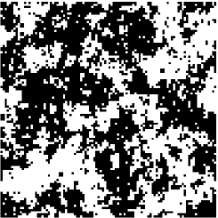
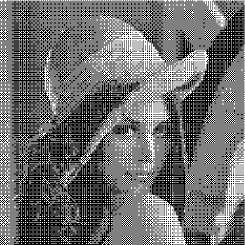
Figure 3: The left panel shows a halftone image converted by the dither method using the uniform threshold $M=2$ from the snapshot from a Gibbs distribution of the $Q=4$ Ising model shown in Fig. 1 (left). The center panel shows a halftone image obtained by the dither method using the $2\times 2$ Bayer-type threshold array from the same snapshot. The right panel shows a halftone image converted by the dither method using the $4\times 4$ Bayer-type threshold array from the 256-level standard image Lenna with $400\times 400$ pixels shown in Fig. 1 (right).

In the Bayesian inverse digital halftoning, we attempt to restore the original grayscale image from a given halftone image by means of the so-called maximizer of posterior marginal (MPM for short) estimate. Then, we define $\{z\}=\{z_{x,y}=0,\cdots,Q-1|x,y=0,\cdots,L-1\}$ as an estimate of the original image $\{\xi\}$ arranged on the square lattice and reconstruct the grayscale image on the bases of maximizing the following posterior marginal probability:

$$\hat{z}_{x,y} = \arg\max_{z_{x,y}}\sum_{\{z\}\not=z_{x,y}}{\rm Pr}(\{z\}|\{\tau\})=\arg\max_{z_{x,y}}{\rm Pr}\left(z_{x,y}|\{\tau\}\right),$$ (4)

where the summation $\sum_{z_{x,y}\neq\{z\}}(\cdots)$ runs over all pixels except for the $(x,y)$-th and the posterior probability $P(\{z\}|\{\tau\})$ is given by the Bayes formula:

$${\rm Pr}\left(\{z\}|\{\tau\}\right)=\frac{{\rm Pr}\left(\{z\}\right){\rm Pr}\left(\{\tau\}|\{z\}\right)}{\sum_{\{z\}}{\rm Pr}\left(\{z\}\right){\rm Pr}\left(\{\tau\}|\{z\}\right)}$$ (5)

In this study, following Stevenson [16], we assume that the likelihood might have the same form as the halftone process of the dither method, namely,

$$P\left(\{\tau\}|\{\xi\}\right)=\Pi_{(x,y)}\delta\left(\tau_{x,y},\theta\left(z_{x,y}-M_{x,y}\right)\right),$$ (6)

where $\delta(a,b)$ denotes a Kronecker delta and we should notice that the information on the threshold array $\{M\}$ is available in addition to the halftone image $\{\tau\}$. Then, we choose the model of the true prior as

$${\rm Pr}(\{z\})=\frac{1}{Z_{m}}\exp\left[-\frac{J}{T_{m}}\sum_{\rm n.n.}\left(z_{x,y}-z_{x^{{}^{\prime}},y^{{}^{\prime}}}\right)^{2}\right],$$ (7)

where $Z_{\rm m}$ is a normalization factor. $J$ and $T$ are the so-called hyper-parameters. It should be noted that one can construct the Bayes-optimal solution if we assume that the model prior has the same form as the true prior, namely, $J=J_{s}$ and $T_{m}=T_{s}$ (what we call, Nishimori line in the research field of spin glasses [1]).

From the viewpoint of statistical mechanics, the posterior probability ${\rm Pr}(\{z\}|\{\tau\})$ generates the equilibrium states of the ferromagnetic Q-Ising model whose Hamiltonian is given by

$$H\left(\{z\}\right)=J\sum_{\rm n.n.}\left(z_{x,y}-z_{x^{\prime},y^{\prime}}\right)^{2},$$ (8)

under the constraints

$$\forall_{x,y}\,\,\,\,\,\,\,\,\tau_{x,y}=\theta\left(z_{x,y}-M_{x,y}\right).$$ (9)

Obviously, the number of possible spin configurations that satisfy the above constraints (9) is evaluated as $\prod_{(x,y)}|Q\tau_{x,y}-M_{x,y}|$ and this quantity is exponential order such as $\sim{\alpha}^{L^{2}}$ ($\alpha$: a positive constant). Therefore, the solution $\{z\}$ to satisfy the constraints (9) is not unique and this fact makes the problem very hard. To reduce the difficulties, we consider the equilibrium state generated by a Gibbs distribution of the ferromagnetic Q-Ising model with the constraints (9) and increase the parameter $J$ gradually from $J=0$. Then, we naturally expect that the system stabilizes the ferromagnetic Q-Ising configurations due to a kind of the regularization term (8). Thus, we might choose the best possible solution among a lot of candidates satisfying (9).

¿From the view point of statistical mechanics, the MPM estimate is rewritten by

$$\hat{z}_{x,y} = \Theta_{Q}(\langle z_{x,y}\rangle),\,\,\,\,\langle z_{x,y}\rangle=\sum_{z}z_{x,y}{\rm Pr}(\{z\}|\{\tau\})$$ (10)

where $\Theta_{Q}(\cdots)$ is the Q-generalized step function defined by

$$\theta_{Q}(x) = \sum_{k=0}^{Q-1}k{\Biggr{\{}}\theta\left(x-\left(k-\frac{1}{2}\right)\right)-\theta\left(x-\left(k+\frac{1}{2}\right)\right){\Biggr{\}}}.$$ (11)

Obviously, $\langle z_{x,y}\rangle$ is a local magnetization of the system described by (8) under (9).

2.1 Average case performance measure

To investigate the performance of the inverse halftoning, we evaluate the mean square error which represents the pixel-wise similarity between the original and restored images. Especially, we evaluate the average case performance of the inverse halftoning through the following averaged mean square error

$$\sigma=\frac{1}{Q^{2}L^{2}}\sum_{\{\xi\}}{\rm Pr}\left(\{\xi\}\right)\sum_{(x,y)}\left(\hat{z}_{x.y}-\xi_{x,y}\right)^{2}.$$ (12)

We should keep in mind that the $\sigma$ gives zero if all restored images are exactly the same as the corresponding original images.

3 Results

In this section, we first investigate the statistical properties of our approach to the inverse halftoning for a set of snapshots from a Gibbs distribution of the ferromagnetic Q-Ising model via computer simulations. We next analytically evaluate the performance for the infinite-range model. Finally, we check the usefulness of our approach for the realistic images, namely, the 256-levels standard image Lenna.

3.1 Monte Carlo simulation

We first carry out Monte Carlo simulations for a set of halftone images, which are obtained from the snapshots from a Gibbs distribution of the ferromagnetic $Q=4$ Ising model with $100\times 100$ pixels by the uniform threshold $M_{x,y}=2\,\,(\forall_{x,y})$ and the $2\times 2$ Bayer-type threshold arrays as shown in Fig. 2. In order to clarify the statistical performance of our method, we reveal the hyper-parameters $J$ and $T_{m}$ dependence of the averaged mean square error $\sigma$.

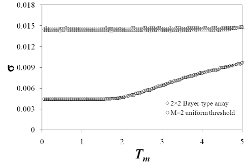
Figure 4: The mean square error as a function of $T_{m}$. The original image is a snapshot from a Gibbs distribution of the $Q=4$ ferromagnetic Ising model with $100\times 100$ pixels and $T_{s}=1.0$, $J_{s}=1$ and $J=1$. The halftone images are obtained by the uniform and $2\times 2$ Bayer-type arrays.

We plot the results in Fig. 4. These figures show that the present method achieves the best possible performance under the Bayes-optimal condition, that is, $J=J_{s}$ and $T_{m}=T_{s}$. We also find from Fig. 4 (the lower panel) that the limit $T_{m}\to\infty$ leading up to the MAP estimate gives almost the same performance as the Bayes-optimal MPM estimate.

This fact means that it is not necessary for us to take the $T_{\rm m}\rightarrow 0$ limit when we carry out the inverse halftoning via simulated annealing.

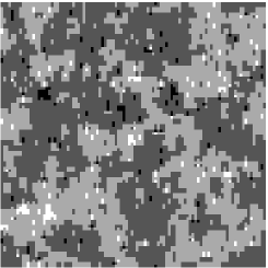
Figure 5: The left panel shows a $Q=4$ grayscale image restored by the MPM estimate from the halftone image shown in Fig. 3 (left). The center panel shows a $Q=4$ grayscale image restored by the MPM estimate from the halftone image shown in Fig. 3 (center). The right panel shows a $Q=256$ grayscale image restored by the MPM estimate from the halftone image shown in Fig. 3 (right).

From the restored image in Fig. 5 (center), it is actually confirmed that the present method effectively works for the snapshot of the ferromagnetic Q-Ising model.

It should be noted that the mean square error evaluated for the $2\times 2$ Bayer-type array is larger than that for the $M=2$ uniform threshold. This result seems to be somewhat counter-intuitive because the halftone image shown in the center panel of Fig. 3 seems to be much closer to the original image, in other words, is much informative to retrieve the original image than the halftone image shown in the left panel of the same figure. However, it could be understood as follows. The shape of each ‘cluster’ appearing in the original image (see the left panel of Fig. 1) remains in the halftone version (the left panel of Fig. 3), whereas, in the halftone image (the center panel of Fig. 3), such structure is destroyed by the halftoning process via the $2\times 2$ Bayer-type array. As we found, in a snapshot of the ferromagnetic Q-Ising model at the inverse temperature $J_{s}/T_{s}=1$, the large size clusters are much more dominant components than the small isolated pixels. Therefore, the averaged mean square error is sensitive to the change of the cluster size or the shape, and if we use the constant threshold mask to create the halftone image, the shape of the cluster does not change, whereas the high-frequency components vanish. These properties are desirable for us to suppress the increase of the averaged mean square error. This fact implies us that the averaged mean square error for the $2\times 2$ Bayer-type is larger than that for the constant mask array and the performance is much worse than expected.

3.2 Analysis of the infinite-range model

In this subsection, we check the validity of our Monte Carlo simulations, namely, we analytically evaluate the statistical performance of the present method for a given set of the snapshots from a Gibbs distribution of the ferromagnetic Q-Ising model in which each spin variable is located on the vertices of the complete graph. For simplicity, we first transform the index from $(x,y)$ to $i$ so as to satisfy $i=x+Ly+1$. Then, the new index $i$ runs from $i=1$ to $L^{2}-1=N$. For this new index of each spin variable, we consider the infinite-range version of true prior and the model as

$${\rm Pr}\left(\{\xi\}\right) = \frac{{\rm e}^{-\frac{\beta_{\rm s}}{2N}\sum_{i<j}(\xi_{i}-\xi_{j})^{2}}}{Z_{\rm s}},\,\,\,{\rm Pr}\left(\{z\}\right)=\frac{{\rm e}^{-\frac{\beta_{\rm m}}{2N}\sum_{i<j}(z_{i}-z_{j})^{2}}}{Z_{\rm m}}$$ (13)

where the scaling factors $1/N$ appearing in front of the sums $\sum_{i<j}(\cdots)$ are needed to take a proper thermodynamic limit. We also set $\beta_{\rm s}\equiv J_{\rm s}/T_{\rm s}$ and $\beta_{\rm m}\equiv J/T_{\rm m}$ for simplicity. Obviously, the thermodynamics of the system $\{\xi\}$ is determined by the following magnetization:

$$m_{0} \equiv \frac{1}{N}\sum_{i=1}^{N}\xi_{i}=\frac{\sum_{\xi=0}^{Q-1}\xi\exp[2\beta_{s}m_{0}\xi-\beta_{s}{\xi}^{2}]}{\sum_{\xi=0}^{Q-1}\exp[2\beta_{s}m_{0}\xi-\beta_{s}{\xi}^{2}]}.$$ (14)

On the other hand, the magnetization for the system $\{z\}$ having disorders $\{\tau\}$ and $\{\xi\}$ is given explicitly as

$$m \equiv \frac{1}{N}\sum_{i=1}^{N}z_{i}=\frac{\sum_{\xi=0}^{Q-1}\left(\frac{\sum_{z=0}^{Q-1}z\,{\rm e}^{2\beta_{m}mz-\beta_{m}z^{2}}\delta(\theta(\xi-M),\theta(z-M))}{\sum_{z=0}^{Q-1}{\rm e}^{2\beta_{m}mz-\beta_{m}z^{2}}\delta(\theta(\xi-M),\theta(z-M))}\right){\rm e}^{2\beta_{s}m_{0}\xi-\beta_{s}{\xi}^{2}}}{\sum_{\xi=0}^{Q-1}{\rm e}^{2\beta_{s}m_{0}\xi-\beta_{s}{\xi}^{2}}}.$$

Then, the average case performance is determined by the following averaged mean square error:

$$\sigma \equiv \frac{1}{NQ^{2}}\sum_{i=1}^{N}\{\xi_{i}-\Theta_{Q}(\langle z_{i}\rangle)\}^{2}$$

$$= \frac{\sum_{\xi=0}^{Q-1}\left\{\xi-\Theta_{Q}\left(\frac{\sum_{z=0}^{Q-1}z\,{\rm e}^{2\beta_{m}mz-\beta_{m}z^{2}}\delta(\theta(\xi-M),\theta(z-M))}{\sum_{z=0}^{Q-1}{\rm e}^{2\beta_{m}mz-\beta_{m}z^{2}}\delta(\theta(\xi-M),\theta(z-M))}\right)\right\}^{2}{\rm e}^{2\beta_{s}m_{0}\xi-\beta_{s}{\xi}^{2}}}{Q^{2}\sum_{\xi=0}^{Q-1}{\rm e}^{2\beta_{s}m_{0}\xi-\beta_{s}{\xi}^{2}}}$$

Solving these self-consistent equations with respect to $m_{0}$ (14) and $m$ (3.2), we evaluate the statistical performance of the present method through the quantity $\sigma$ (LABEL:eq:sigma) analytically.

As we have estimated using the Monte Carlo simulation, we estimate how the mean square error depends on the hyper-parameter $T_{m}$ for the infinite-range version of our model when we set to $Q=8$, $J_{s}=1$, $T_{s}=1$, $M=3.5\,(=(Q-1)/2),4.5$ and $J=1$.

We find from Figs. 6 (a) and (b) that the mean square error takes its minimum in the wide range on $T_{m}$ including the Bayes-optimal condition $T_{m}=T_{s}\,(=1)$. Here, we note that $m=m_{0}\,(=3.5)$ holds under the Bayes-optimal condition, $T_{m}=T_{s}$ for both cases of $M=3.5$ and $M=4.5$, which is shown in Fig. 7. From this fact, we might evaluate the gap $\Delta$ between the lowest value of the mean square error and the second lowest value obtained at the higher temperature than $T_{s}$ as follows.

$$\Delta \simeq \frac{\sum_{\xi=0}^{Q-1}(\xi-m_{0})^{2}{\rm e}^{2\beta_{s}m_{0}\xi-\beta_{s}\xi^{2}}}{Q^{2}\sum_{\xi=0}^{Q-1}{\rm e}^{2\beta_{s}m_{0}\xi-\beta_{s}\xi^{2}}}-\frac{\sum_{\xi=0}^{Q-1}(\xi-m_{0}-1)^{2}{\rm e}^{2\beta_{s}m_{0}\xi-\beta_{s}\xi^{2}}}{Q^{2}\sum_{\xi=0}^{Q-1}{\rm e}^{2\beta_{s}m_{0}\xi-\beta_{s}\xi^{2}}}$$ (17)

$$= \frac{\sum_{\xi=0}^{Q-1}(2\xi-2m_{0}+1){\rm e}^{2\beta_{s}m_{0}\xi-\beta_{s}\xi^{2}}}{Q^{2}\sum_{\xi=0}^{Q-1}{\rm e}^{2\beta_{s}m_{0}\xi-\beta_{s}\xi^{2}}}=\frac{1}{Q^{2}}$$

For example, for $Q=8$, we evaluate the gap as $\Delta=(8)^{-2}=0.00156$ and this value agree with the result shown in Fig. 6.

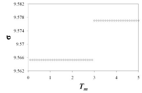
(a)

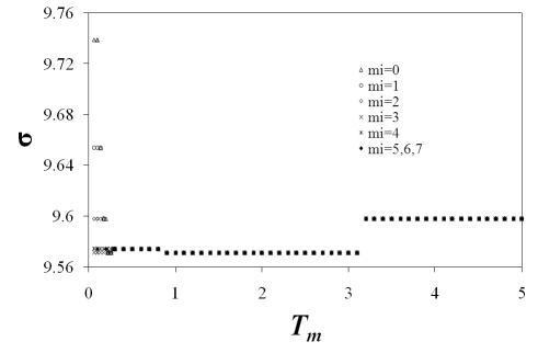
(b)

Figure 6: (a) The mean square error as a function of the parameter $T_{m}$ when $Q=8$, $T_{s}=1$, $J_{s}=1$, $M=(Q-1)/2$ and $J=1$, (b) The mean square error as a function of the parameter $T_{m}$ when $Q=8$, $T_{s}=1$, $J_{s}=1$, $M=4.5\not=(Q-1)/2$ and $J=1$. The value $m_{\rm i}$ for each line caption denotes the initial condition of the magnetization $m$ to find the locally stable solution.

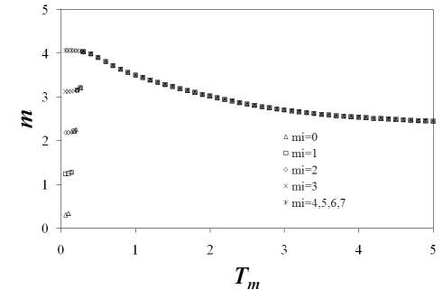
Figure 7: The magnetization $m$ as a function of the parameter $T_{m}$ when $Q=8$, $T_{s}=1$, $J_{s}=1$, $M=4.5\not=(Q-1)/2$ and $J=1$.

From Figs. 6 and 7, we also find that the range of $T_{m}$ in which the mean square error takes the lowest value coincides with the range of temperature $T_{m}$ for which the magnetization satisfies $m(T_{m})=m(T_{s}=1)\pm 1=3.5\pm 1$ as shown in Fig. 7. This robustness for the hyper-parameter selecting is one of the desirable properties from the view point of the practical use of our approach.

Moreover, the above evaluations might be helpful for us to deal with the inverse halftoning from the halftoned image of the standard image with confidence. In fact, we are also confirmed that our method is practically useful from the resulting image shown in Fig. 5 (right) having the mean square error $\sigma=0.002005$.

4 Summary

In this paper, we investigated the condition to achieve the Bayes-optimal performance of inverse halftoning by making use of computer simulations and analysis of the infinite range model. We were also confirmed that our Bayesian approach is useful even for the inverse halftoning from the binary dots obtained from standard images, in the wide range on $T_{m}$ including the Bayes-optimal condition, $T_{m}=T_{s}$. We hope that some modifications of the prior distribution might make the quality of the inverse halftoning much better. It will be our future work.

References

- [1] H. Nishimori, Statistical Physics of Spin Glasses and Information Processing: An Introduction, Oxford University Press, London (2001).
- [2] J. Besag, J. Roy. Stat. Soc. B 48, no. 3, 259 (1986).
- [3] R.C. Gonzales and R.C. Woods, Digital Image Processing, Addison Wesley, Reading, MA. (1992).
- [4] J.M. Pryce and D. Bruce, J. Phys. A: Math. Gen. 28, 511(1995).
- [5] G. Winkler, Image Analysis, Random fields and Markov Chain Monte Carlo Methods, Springer (2002).
- [6] K. Tanaka, J. Phys. A: Math. Gen. 35, R81 (2002).
- [7] R. Ulichney, Digital Halftoning, MIT Press, Massachusetts (1987).
- [8] B.E. Bayer, ICC CONF. RECORD, 11 (1973).
- [9] R. W. Floyd and L. Steinberg, SID Int. Sym. Digest of Tech. Papers, 36 (1975).
- [10] C.M. Miceli and K.J. Parker, J. Electron Imaging 1, 143(1992).
- [11] P.W. Wong, IEEE Trans. on Image Processing 4, 486(1995).
- [12] S.D. Cabrera, K. Iyer, G. Xiang and V. Kreinovich: On Inverse Halftoning: Computational Complexity and Interval Computations, 2000 Conference on Information Science and Systems, The Johns Hopkins University, March 16-18 (2005).
- [13] M. Discepoli and I. Greace, Lecture Note on Computer Science 3046, 388 (2004).
- [14] S. Kirkpatrick, C.D. Gelatt and M.P. Vecchi, Science 220, 671 (1983).
- [15] S. Geman and D. Geman, IEEE Trans. Pattern Anal. and Mach. Intel. 11, 721 (1989).
- [16] R.L. Stevenson, IEEE 6, 574(1997).
- [17] D. Boll, H. Rieger and G.M. Shim, J. Phys. A: Math. Gen. 27, 3411 (1994).
- [18] Y. Saika and J. Inoue, submitted to Journal of Information Processing Society of Japan (in Japanese) (2008).