Sudden death, birth and stable entanglement in a two-qubit Heisenberg XY spin chain

Abstract

Taking the decoherence effect due to population relaxation into account, we investigate the entanglement properties for two qubits in the Heisenberg XY interaction and subject to an external magnetic field. It is found that the phenomenon of entanglement sudden death (ESD) as well as sudden birth(ESB) appear during the evolution process for particular initial states. The influence of the external magnetic field and the spin environment on ESD and ESB are addressed in detail. It is shown that the concurrence, a measure of entanglement, can be controlled by tuning the parameters of the spin chain, such as the anisotropic parameter, external magnetic field, and the coupling strength with their environment. In particular, we find that a critical anisotropy constant exists, above which ESB vanishes while ESD appears. It is also notable that stable entanglement, which is independent of different initial states of the qubits, occurs even in the presence of decoherence.

Entanglement, one of the essential features in quantum mechanics, has been generally believed to be a basic resource in quantum information.^[1-4] In order to realize quantum-information processors, stability of entanglement of quantum subsystems is one of the most important premises that deserves much attention. The entanglement has been extensively studied for various systems including cavity-QED,^[5,6] Ising model,^[7] isotropic and anisotropic Heisenberg chains.^[8-11] In particular, the Heisenberg spin chain has been used to construct a quantum computer in many physical systems such as quantum dots, nuclear spins, electronic spins and optical lattice based systems. By proper encoding, the Heisenberg interaction alone can support universal quantum computation.^[12,13] Therefore, the study of entanglement properties of Heisenberg spin chain has received much attention in the context of quantum information science. However, in the real world, the environmental-induced decoherence will destroy quantum superposition and entanglement, and thus ruin the encoded quantum information. Counter-intuitively to conventional qubit decoherence theory, Yu and Eberly^[14] have shown that entanglement may decrease abruptly to zero in a finite time due to the influence of quantum noise, this striking phenomenon is the so-called entanglement sudden death (ESD). Opposite to the currently extensively discussed ESD, entanglement sudden birth (ESB) is the creation of entanglement where the initially unentangled qubits can be entangled after a finite evolution time.^[15] Recently, many theoretical works^[16-21] investigated the disentanglement dynamics in cavity-QED (Jaynes-Cummings and Tavis-Cummings model) and spin chain. In [17], ESD induced by the effect of nonzero initial photon number in the cavity was demonstrated via the Tavis-Cummings model. In [18], it has been shown that atomic ESD always occurs if ithe atomic initial state is sufficiently impure and/or the cavity photon number is nonzero. The explicit expression for the ESD time for various entangled states has presented in [21]. In particular, ESD has been experimentally observed recently both in photonic qubits^[22] and in atomic ensemble systems.^[23]

Although the environmental induced effect is not what we desired in most cases, it has been shown that entanglement between two or more subsystems may be induced by their collective interaction with a common environment. A stable entangled state, in which once qubits become entangled they will never be disentangled, was also demonstrated in [24,25]. In this Letter, we present an exact calculation of the entanglement dynamics between two qubits coupling with a common environment at zero temperature. The two qubits interact via a Heisenberg XY interaction and are subject to an external magnetic field. Apart from the important link to quantum information processing, a deeper understanding of disentanglement is also expected to provide new insights into quantum fundamentals, particularly for quantum measurement and quantum to classical transitions. The main purpose and motivation of the present study is try to answer the following question: what happens to the qubits entanglement when we consider different system parameters and initial state in the absence or presence of the decoherence? An important result is that ESD and ESB appear simultaneously and is sensitive to the initial state as well as the system parameters. Meanwhile, a critical anisotropy constant exists, above which ESB vanishes while ESD appears. Moreover, it is also shown that the decoherence due to population relaxation will always lead to stable entanglement irrespective of the initial entangled state of the qubits.

The Hamiltonian for an anisotropic N-qubit Heisenberg chain with only nearest-neighbor interactions can be written as

$$H=\sum^{N}_{i=1}(J_{x}S_{i}^{x}S_{i+1}^{x}+J_{y}S_{i}^{y}S_{i+1}^{y}+J_{z}S_{i}^{z}S_{i+1}^{z})$$ (1)

Here we consider an anisotropic two-qubit Heisenberg XY system coupled to an environment in an external magnetic field $\omega$ along the z-axis, the corresponding Hamiltonian reads

$$H=J(S_{1}^{+}S_{2}^{-}+S_{1}^{-}S_{2}^{+})+\Delta(S_{1}^{+}S_{2}^{+}+S_{1}^{-}S_{2}^{-})+\omega(S_{1}^{z}+S_{2}^{z})$$ (2)

where $J=(J_{x}+J_{y})/2$, $\Delta=(J_{x}-J_{y})/2$, and $S^{\pm}=S^{x}\pm iS^{y}$ are the spin raising and lowering operators, the parameter $\Delta$ describes the spatial anisotropy of the spin-spin interaction. The anisotropy parameter can be controlled by varying $J_{x}$ and $J_{y}$, which may possibly be achieved for an optical lattice system^[26], the effective external magnetic field is defined by the energy levels of our qubits. The description of the time evolution of an open system is provided by the master equation, which can be written most generally in the Lindblad form with the assumption of weak system-reservoir coupling and Born-Markov approximation. The Lindblad equation for our case thus reads

$$\frac{d\rho}{dt}=-i[H,\rho]+\gamma\sum\limits_{j=1,2}[S_{j}^{-}\rho S_{j}^{+}-\frac{1}{2}\left\{S_{j}^{+}S_{j}^{-},\rho\right\}]$$ (3)

where $\gamma$ is the relaxation rate of the qubits and we have assumed them to be the same; the assumption is reasonable provided the interaction does not significantly alter the energy level separations. $\{\}$ means anticommutator.

Firstly, the solution of Eq. (3) depends on the initial state of the qubits, and we assume that the initial state of the system is in a general form $\cos\theta|\downarrow\downarrow\rangle+\sin\theta|\uparrow\uparrow\rangle$. We note that, for the class of the initial states considered here, the solution of Eq.(3) has the matrix form

$$\rho=\left(\begin{array}[]{cccc}\rho_{1,1}&0&0&\rho_{1,4}\\ 0&\rho_{2,2}&\rho_{2,3}&0\\ 0&\rho_{3,2}&\rho_{3,3}&0\\ \rho_{4,1}&0&0&\rho_{4,4}\end{array}\right)$$ (8)

in the two-qubit product state basis of $\{\left|\uparrow\uparrow\right\rangle,\left|\uparrow\downarrow\right\rangle,\left|\downarrow\uparrow\right\rangle,\left|\downarrow\downarrow\right\rangle\}$.

Since decoherence process leads the pure quantum system state to mixed states, we use the concurrence as a measure of entanglement. The concurrence $C=0$ corresponds to a separable state and $C=1$ to a maximally entangled state. Nonzero concurrence means that the two qubits are entangled. Using Wootters formula,^[26] for a system described by the above density matrix in Eq. (4), the concurrence is

$$C(\rho)=\max(0,\lambda_{1}-\lambda_{2}-\lambda_{3}-\lambda_{4})$$ (9)

where $\lambda_{1}$, $\lambda_{2}$, $\lambda_{3}$, $\lambda_{4}$ are the eigenvalues in a decreasing order of the spin-flipped density operator $R$ defined by $R=\sqrt{\sqrt{\rho}\tilde{\rho}\sqrt{\rho}}$ with $\tilde{\rho}=(\sigma_{y}\otimes\sigma_{y})\rho^{\ast}(\sigma_{y}\otimes\sigma_{y})$, $\tilde{\rho}$ denotes the complex conjugate of $\rho$, $\sigma_{y}$ is the usual Pauli matrix. Then the concurrence can be expressed as

$$C=max[0,2(\sqrt{\rho_{23}\rho_{23}}-\sqrt{\rho_{11}\rho_{44}}),2(\sqrt{\rho_{14}\rho_{41}}-\sqrt{\rho_{22}\rho_{33}})]$$ (10)

In the following, we use this formalism to investigate the entanglement dynamics and decoherence under different system parameters, such as the anisotropic parameter, external magnetic field, for several different initial cases: the disentangled of the two qubits ($\theta=0,\theta=\frac{\pi}{2}$), not maximal entangled state ($\theta=\frac{\pi}{8}$) and maximal entangled state ($\theta=\frac{\pi}{4},\theta=\frac{3\pi}{4}$).

In Figs.1 and 2, the time evolution of the concurrence is plotted for various values of the external magnetic field parameter $\Omega$ with and without the decoherence when the qubits are initially in the different initial state. From Figs.1(a) and 1(c), one can find that the entanglement evolves periodically in the absence of the decoherence. If there is no magnetic field, we can see that unentangled initial state periodically generates maximally entangled states; while the maximally entangled initial state does not evolve in time as shown in Fig.1(c), as it is an eigenvector of the Hamiltonian in the absence of the surrounding environment. The solid line represents result when the control field is turned off, the dashed, dotted and dash-dotted lines correspond to different control field strength $\omega=0.2,0.6,$ and $1.0$, respectively. In contrast to the solid line in Fig.1(a), once the magnetic field is given, the amplitude of these oscillations decreases with the increase of the external magnetic field. It makes slow oscillation around the maximal value of concurrence, $C=1$. Similar behaviours to those in Figs.1(a) and 2(c) are shown in Figs.2(a) and 2(c). From Fig.1(b), we can see that the two-qubit state can evolve into a stationary entangled state under the collective decay from initial unentangled state. In other words, decoherence drives the qubits into a stationary entangled state instead of completely destroying the entanglement. Moreover, the stationary entanglement of two qubits increases with the decrease of the external magnetic field. Therefore, this can provide us a feasible way to manipulate and control the entanglement by changing the external magnetic field. Contrarily, Figures 1(d) and 2(d) show that as the external magnetic field increases the entanglement of two qubits can fall abruptly to zero, and will recover after a period of time. Therefore, the ESD appears and is related to both the initial state and the external magnetic field. Even though the initial system has the same entanglement, different evolution will appear. When the two spins are initially prepared in their excited state, i.e. $\theta=\frac{\pi}{2}$ , the result is quite different from that of Fig.1(b). The concurrence versus parameter $t$ is plotted in Fig. 2(b), indicating a threshold value of parameter $t$, only above which concurrence begins to be nonzero, i.e. the quantum correlation starts to appear. This is the so-called ESB and the delayed time for the appearance of ESB increases with the increasing of the strength of external magnetic field.

At this stage, we turn to study the influence of anisotropy effect of the system on the entanglement dynamics. Figure 3 illustrates the time evolution of the concurrence for different values of the anisotropy constant $\Delta$ with decoherence effect. By comparing Fig.3(c) and 3(d), it is observed that at a fixed external magnetic field, a critical anisotropy constant exists, above which ESB vanishes while ESD appears. It is the anisotropy of interaction that leads to considerable difference in entanglement evolution, hence entanglement is rather sensitive to any small change of the system anisotropy. That is to say by adjusting the anisotropic constant alone one can also obtain both ESD and ESB. Another important property revealed by Fig.3(c) is that ESD occurs twice with the increase of the system anisotropy. In the case of weak external magnetic field and strong anisotropy interaction, as we show in the dash-dotted lines of Figs.3(a), 3(b) and 3(c), concurrence actually goes abruptly to zero in a finite time and remains zero thereafter, i.e., the ESD will always survive in a strong anisotropic interaction. At strong control field in Fig.3(d), the system loses its entanglement completely for a short period of time, and then it is entangled again some time later. Thus the lifetime of ESD can be controlled in our model by applying local external magnetic field. Despite the presence of decoherence, the results in Fig. 4 show that the concurrence reaches the same steady value, after some oscillatory behaviour, for a given set of system parameters regardless of the initial state of the system. At $T=0$, the corresponding steady concurrence is found to be

$$C_{s}=\frac{2\Delta\sqrt{4\omega^{2}+\Delta^{2}}-2\Delta^{2}}{4(\omega^{2}+\Delta^{2})+\gamma^{2}}$$ (11)

The steady-state concurrence is seen to depend on the system parameters $\omega,\Delta$, and $\gamma$ while independent of the $J$ and the initial entangled state of the qubits.

In summary, we have presented an analytic solution for the evolution of entanglement for different initial system states. It is found that ESD and ESB appear simultaneously, depending on the initial state, the anisotropic parameter, external magnetic field, and the coupling strength with the environment. A stable entanglement, controllable by the values of the system parameters, will always be obtained for zero or finite. Our results will shed light on understanding of entanglement dynamics of quantum systems with environmental effect as well as the ESD and ESB in a correlated environment.
We thank Z-Y Xue for his reading of the manuscript.
Note added- After the completion of this paper, C. E. López brought to our attention the Letter published in [28] and we thank C. E. López for useful discussions.

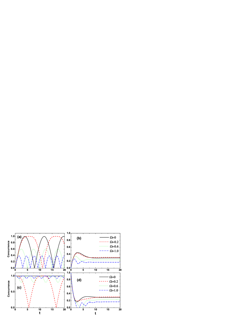
Figure 1: The time evolution of the concurrence for various values of the external magnetic field parameter $\Omega$ with $\Delta=0.2$ when the qubits are initially in different initial state. (a)$\theta=0,\gamma=0$, (b)$\theta=0,\gamma=0.5$, (c)$\theta=\frac{\pi}{4},\gamma=0$, (d)$\theta=\frac{\pi}{4},\gamma=0.5$.

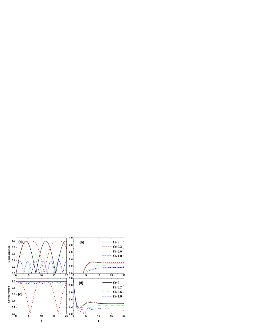
Figure 2: The time evolution of the concurrence for various values of the external magnetic field parameter $\Omega$ with $\Delta=0.2$ when the qubits are initially in different initial state. (a)$\theta=\frac{\pi}{2},\gamma=0$, (b)$\theta=\frac{\pi}{2},\gamma=0.5$, (c)$\theta=\frac{3\pi}{4},\gamma=0$, (d)$\theta=\frac{3\pi}{4},\gamma=0.5$.

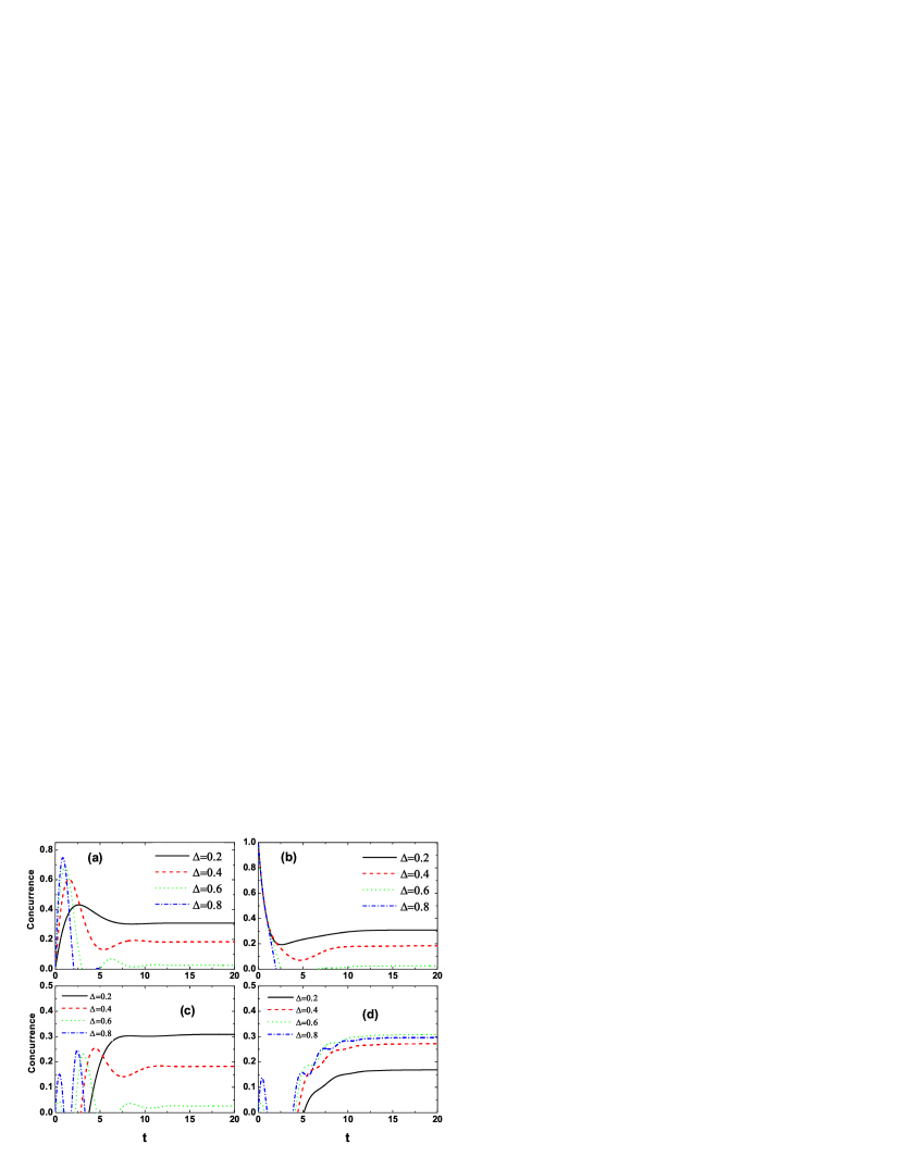
Figure 3: The time evolution of the concurrence for various values of the anisotropic parameter with $\gamma=0.5$ when the qubits are initially in different initial state. (a)$\theta=0,\Omega=0.2$, (b)$\theta=\frac{\pi}{4},\Omega=0.2$, (c)$\theta=\frac{\pi}{2},\Omega=0.2$, (d)$\theta=\frac{\pi}{2},\Omega=1.0$

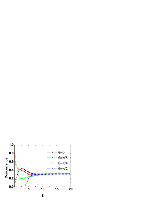
Figure 4: The time evolution of the concurrence with $\Omega=0.2,\Delta=0.2,\gamma=0.5$ when the qubits are initially in different initial state.

References

-
(1)
Bennett C H et al 1993 Phys. Rev. Lett. 70 1895
Xue Z Y, Yang M, Yi Y M, and Cao Z L 2006 Opt. Commun. 258 315 -
(2)
Wei H, Deng Z J, Zhang X L and Feng M 2007 Phys. Rev. A 76
054304
Wei H, Fang R R, Liu J B et al 2008 J. Phys. B41 085506 -
(3)
Xue Z Y, Yi Y M, and Cao Z L 2007 Physica A 374
119
Xue Z Y, Yi Y M, and Cao Z L 2006 J. Mod. Opt. 53 2725 - (4) Grover L 1998 Phys. Rev. Lett. 80 4329
- (5) Zheng S B and Guo G C 2000 Phys. Rev. Lett. 85 2392
- (6) Liu T K, Cheng W W, Shan C J et al 2007 Chin. Phys. 16 3697
- (7) Pang C Y and Li Y L 2006 Chin. Phys. Lett. 23 3145
- (8) Wang X G 2001 Phys. Rev. A 64 012313; 2002 66 044305; 2002 66 034302
- (9) Zhang G F and Li S S 2005 Phys. Rev. A 72 034302
- (10) Zhou L, Song H S, Guo Y Q and Li C 2003 Phys. Rev. A 68024301
- (11) Shan C J, Cheng W W, Liu T K, Huang Y X and Li H 2008 Chin. Phys. Lett. 25 817; Chin. Phys. 17 0794; Cheng W W, Huang Y X, Liu T K and Li H 2007 Physica E 39 150
- (12) Christandl M, Datta N, Ekert A and Landahl A J 2004 Phys. Rev. Lett. 92 187902
- (13) Mohseni M and Lidar D A 2005 Phys. Rev. Lett. 94 040507
- (14) Yu T and Eberly J H 2004 Phys. Rev. Lett. 93 140404
- (15) Ficek Z and Tanas R 2008 Phys. Rev. A 77 054301
- (16) Yu T and Eberly J H 2006 Phys. Rev. Lett. 97 140403
- (17) Shan C J, Xia Y J 2006 Acta. Phys. Sin. 55 1585
- (18) Man Z X, Xia Y J and An N B 2008 J. Phys. B 41 085503
- (19) Yang Q, Yang M, Cao Z L et al 2008 Chin. Phys. Lett. 25 825
- (20) Jing J, Lü Z G and Yang G H 2007 Phys. Rev. A 76 032322
- (21) Ikram M, Li Fl and Zubairy M S 2007 Phys. Rev. A 75 062336
- (22) Almeida M P et al 2007 Sience 316 579
- (23) Laurat J et al 2007 Phys. Rev. Lett. 99 180504
- (24) Hartmann L, Dür W and Briegel H J 2007 Phys. Rev. A 74 052304
- (25) Abliz A et al 2006 Phys. Rev. A 74 052105
- (26) Sørensen A and Mølmer K 1999 Phys. Rev. Lett. 83 2274; Duan L M, Demler E, Lunkin M D 2003 Phys. Rev. Lett. 91 090402
- (27) Wooters W K 1998 Phys. Rev. Lett. 80 2245
- (28) López C E, Romero G, Lastra F, Solano E, and Retamal J C 2008 Phys. Rev. Lett. 101 080503