Practical Coherent Integration with the NPOI

Abstract

In this paper we will discuss the current status of coherent integration with the Navy Prototype Optical Interferometer (NPOI)[1]. Coherent integration relies on being able to phase reference interferometric measurements, which in turn relies on making measurements at multiple wavelengths. We first discuss the generalized group-delay approach, then the meaning of the resulting complex visibilities and then demonstrate how coherent integration can be used to perform very precision measurement of stellar properties. For example, we demonstrate how we can measure the diameter of a star to a precision of one part in 350, and measure properties of binary stars. The complex phase is particularly attractive as a data product because it is not biased in the same way as visibility amplitudes.

1 Introduction

At the 2004 and 2006 SPIE meetings we demonstrated how to coherently integrate NPOI[1] data by fitting a model of the fringes to the raw data and using the fitting parameters to coherently integrate the complex visibilities from individual frames [2, 3]. This discussion was also published in a separate paper [4]. In this paper we take a different approach to fringe tracking which is an extension of the conventional group-delay approach, but including the atmospheric dispersion as well as time-dependence in the group-delay calculation. This is discussed in Section 2. We then discuss the meaning of the resulting coherently integrated complex visibilities, including the phase (Section 4), and the amplitude (Section 5). We then show two examples of how to use complex visibilities for scientific measurements, including an precise diameter measurement (Section 7) and precise measurements on a binary star (Section 8), before concluding.

The Navy Prototype Optical Interferometer (NPOI) [1], located in Flagstaff, AZ, measures fringes by scanning the optical path-difference across several fringe periods (usually between one and eight) and using photon-counting avalanche photo diodes to detect the photons and bin them according to fringe phase at up to 32 different wavelengths in three different spectrographs. This produces a regular array every 2 ms with fringe phase along one dimension and wavelength along the other dimension, making it easy to process the arrays with Fourier-based techniques. For technical reasons the NPOI data has been restricted to 16 wavelength channels in two spectrographs in recent years, and those are the data we will show here. It is important however that NPOI measures many channels (which we will define as approximately ten or more) because it is this multi-wavelength capability which makes coherent integration possible and interesting. Coherent integration consists of two primary steps, as outline in Figure 1. The first step uses the data to estimate the fringe phase whereas the second step uses the estimate of the fringe phase together with the data to produce coherently integrated visibilities, as outline in the next two sections.

Figure 1: An overview of the coherent integration procedure. It consists of two primary steps. The first is the determination of the fringe phase, and the second is the coherent integration using the measured fringe phase.

2 Generalized group-delay fringe finding

The traditional group-delay is defined as the vacuum delay, $d$, which best aligns the fringes in different wavebands. If a delay is applied, a fringe at wavelength $\lambda$ is rotated by

$$\theta=\frac{2\pi d}{\lambda}$$ (1)

We can add the visibilities at different wavelengths,

$$X+iY=\sum_{i}(X+iY)_{i}e^{-\theta_{i}}$$ (2)

where $X$ and $Y$ are the cosine and sine transforms of the photon data, and related to the visibility as $\tilde{V}=\frac{X+iY}{N}$, where $N$ is the total number of photons. The sum is over different wavelength channels. The group-delay is then defined as the value of $d$ which maximizes $\left|X+iY\right|^{2}$. An algorithm similar to this is implemented in the NPOI real-time fringe-tracking system [5], and the best group-delay can be found quickly because it involves a linear search over a single parameter.

We can generalize this simple approach to fringe tracking by including more parameters in Equation 1, allowing them to vary as a function of time, and making the sum in Equation 2 to be over multiple consecutive exposures.

First, a more realistic functional form for the variation of the phase with wavelength should include the dispersive atmosphere,

$$\theta_{i}=\frac{2\pi(d+(n(\lambda_{i})-1)a)}{\lambda_{i}}$$ (3)

We can also include time-variation of the parameters $d$, and $a$. We allow them to vary as Legendre polynomials (which are defined in the interval $[-1;1]$), e.g.

$$d(t-t_{0})=\sum_{i=0}^{n_{d}-1}e_{i}L\left(\frac{2(t-t_{0})}{T}\right)$$

and

$$a(t-t_{0})=\sum_{i=0}^{n_{a}-1}b_{i}L\left(\frac{2(t-t_{0})}{T}\right)$$

Where we are modeling the time-variation of $d$ and $a$ over the time-interval of length $T$. We can then determine a set of parameters, $\{e_{i}\}$ and $\{b_{i}\}$ which best models the wavelength and time-variation of the fringes over a short time-interval.

We find this best set of model parameters by maximizing the quantity $\left|X+iY\right|^{2}$, where

$$X+iY=\sum_{j=1}^{M}\sum_{i=1}^{N}\left(X_{ij}+iY_{ij}\right)e^{-\theta_{ij}}$$

Where $j$ counts time, and $i$ counts wavelengths. Our claim is then that fitting this more complicated fringe phase function to a set of frames can produce a better estimate of the phase of the central frame of the set. We estimate $d_{ij}$ and $a_{ij}$ for the central frame. In this way we estimate $d$ and $a$ for nearly all the data frames in the data sets. We also record the phase $\phi=\angle X+iY$.

3 Coherent integration

To coherently integrate we rotate the individual complex quantities $(X_{ij}+iY_{ij})$ by the angle

$$\theta_{ij}=\frac{2\pi\left(d_{j}+a_{j}(n(\lambda_{i})-1)\right)}{\lambda_{i}}-\phi_{j}$$ (4)

where $i$ counts wavelength, and $j$ counts the frames (exposures) over which we are coherently integrating (typically 10’s of thousands). The coherent integration looks like this

$$X_{i}+iY_{i}=\sum_{j=1}^{M}\left(X_{ij}+Y_{ij}\right)e^{\theta_{ij}}$$ (5)

We also sum the photon counts,

$$N_{i}=\sum_{j=1}^{M}N_{ij}$$

The complex visibility at each wavelength can then be computed as

$$\tilde{V_{i}}=\frac{X_{i}+iY_{i}}{N_{i}}$$

and the squared visibility and visibility phase (at each wavelength) can be computed as

$$V_{i}^{2}=4\frac{X_{i}^{2}+Y_{i}^{2}-N_{i}}{N_{i}^{2}}$$

(assuming Poisson statistics) and

$$\phi_{i}=\tan^{-1}(Y_{i}/X_{i})$$

where one must be careful to consider the quadrant of $\phi_{i}$ for it to range over the full $[0;2\pi[$ range, for example by using the function atan2(Y,X) available in some form in most computer languages. To consider non-Poisson statistics one must replace the subtracted $N$ in Equation 3 with the actual estimated Bias. However, in most practical situations, the bias is smaller than the uncertainty and can thus be ignored. For that reason it is usually not necessary to consider the details of the bias statistics either. Effectively, coherently integrated squared visibilities do not have a bias - at least not one large enough to need to correct, except in cases of extremely small visibility amplitudes.

When coherently integrating it is not possible to coherently integrate on the same data used for fringe tracking. If that is done, a bias similar to the bias in incoherent $V^{2}$ averaging is introduced. We can overcome this problem by sub-dividing the data sets. For example, we can separate the data set into even-numbered channels and odd-numbered channels (as illustrated in Figure 2b), track fringes in each set, and use that information to coherently integrate the channels in the other set. This is a form of wavelength bootstrapping. However it is not very efficient in that for each channel we now only track fringe using half of the available data. A more computationally intensive approach which produces better signal-to-noise ratio is illustrated in Figure 2a, the fringe finding is repeated for each channel, each time leaving out only that channel.

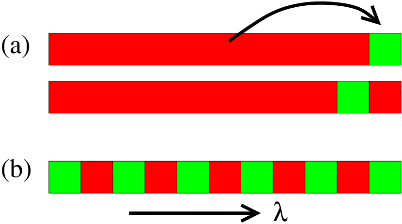
Figure 2: Illustration of two approaches to fringe finding and coherent integration which bootstraps the phase in one wavelength channel from phase measurements in other wavelength channels.

Figure 3: Illustration of the process of phasor rotation and coherent integration. In the top panel are the raw coherent visibilities for 100 short observations of the star $\nu\,\text{Oph}$. In the bottom panel the visibilities have been rotated, and the thick phasor is their average. The circle segment shows the average amplitude of the individual visibilities, demonstrating that phase noise reduces the coherently integrated visibility.

An example of what the coherent integration process looks like is shown in Figure 3. This figure illustrates the rotation and coherent averaging of complex visibilities. In the top panel are plotted the raw coherent visibilities. In the bottom panel are plotted the same visibilities after rotation as well (thick vector) the average of those visibilities. The amplitude of the coherent average is smaller than the average of the amplitudes of the individual complex visibilities, with the difference due to the imperfect rotation of the complex visibilities. This effect of reducing the visibility amplitude when coherently integrating, because of phase noise, will be discussed in Section 5.

4 The coherent phase

Next we consider the phase of the coherently integrated visibilities. Following the simple procedure above, the phase on each baseline is composed of the following components,

$$\phi=\phi_{\text{source}}+\phi_{\text{instr}}+\phi_{\text{atm}}$$ (6)

which are the source phase (the one we are interested in), an instrumental phase caused by mismatch between the two light paths of the interferometer (in particular glass windows), and a residual atmospheric phase. Note that these three phases are additive. Thus, we can determine the instrumental phase plus an arbitrary amount of atmospheric phase by observing a calibrator which has zero source phase. Subtracting the measured phase of a calibrator star thus eliminates the instrumental term, but leaves the atmospheric term. We know the exact form of the atmospheric term, because it looks like Equation 3. Figure 4 shows the instrumental phase recorded from a calibrator star. An important observation is that the phase of the coherently integrated visibilities is not biased like the amplitude is. This means that the raw photon-counting-based uncertainty of the phase is the actual uncertainty. The uncertainty of the phase can be shown to be

$$\sigma_{\phi_{i}}=\frac{1}{\sqrt{2N_{i}V_{i}^{2}}}$$

Where $N_{i}$ is the total number of photons in channel $i$ over the coherently integrated interval, and $V_{i}$ is the raw coherently integrated visibility amplitude.

Figure 4: Example of an instrumental phase measured by observing a calibrator star.

5 The coherent amplitude

The coherent amplitude is reduced due to phase noise in the determination of the rotation phase. As illustrated in Figure 5 coherent integration causes an additional amplitude reduction due to the phase noise in determining the appropriate rotation of the individual phasors.

Figure 5: Illustration of the reduction of the coherently integrated visibility amplitude relative to the raw visibility amplitude. This reduction is due to the finite precision in the determination of rotation phases.

In order to make use of the coherently integrated visibility amplitudes it is necessary to calibrate them and correct for the amplitude-reducing effects of the phase noise. Once this is done, the resulting instrumental visibilities can be calibrated in the usual manner by dividing by the amplitude of a calibrator star. The simplest description of the effect of the phase noise can be based on the distribution of phase errors. If the phase errors, $\Delta\theta$ are distributed according to $f(\Delta\theta)$, then the visibility will be reduced by the factor $\gamma$,

$$\gamma=\int f(\Delta\theta)e^{i\Delta\theta}d\Delta\theta$$

In the case where $f(\Delta\theta)$ is a Gaussian with standard deviation $\sigma_{\theta}$, the integral reduces to

$$\gamma=e^{-\sigma_{\theta}^{2}}$$

If we then assume that a Gaussian is a reasonable model for the phase noise distribution the next question becomes how we measure $\sigma_{\theta}$. Because we measure more than one (at least two) estimate for the fringe phase, as illustrated in Figure 2, we can also estimate the phase noise as the difference between these multiple estimates. However, when doing this it is important that the function used to represent the fringe phase is a true description of the fringe phase with the appropriate number of degrees of freedom, for example the expression in Equation 3 which contains both a vacuum path and an atmosphere path. Figure 6 illustrates how well amplitude calibration can be performed, and the importance of choosing an appropriate model for the fringe phase as a function of wavelength.

Figure 6: Amplitude calibration of coherently integrated squared visibilities. The solid curve is the true instrumental squared visibility. The dotted curve is the coherently integrated squared visibility using a vacuum variation of phase only (Equation 1), whereas the dashed curve uses a model which contains both vacuum and atmosphere (Equation 3). The dot-dashed curve is the correction of the dotted curve, whereas the triple-dot-dashed curve is the correction of the dashed curve.

In Figure 6 the solid curve is the true instrumental squared visibility, which is the target for the calibration of the coherently integrated squared visibilities. The dotted curve represents the coherently integrated squared visibility obtained by finding fringes with a model which tracks only vacuum delay (Equation 1). The dashed curve is the squared visibility coherently integrated when the fringe phase was found using a model which includes both vacuum and atmospheric delay (Equation 3). We notice firs that the simpler model performs marginally better at longer wavelengths, whereas the more complex model performs much better at shorter wavelengths. Because we subdivided the wavelength channels into groups, as illustrated in Figure 2, we can estimate the uncertainty with which we have estimated the phase as the difference between the estimates of these different groups, and use that with Equation 5 to apply a correction.

The dot-dashed curve is the corrected squared visibility for the case where a pure vacuum model was use for tracking the fringes. We can see that at the red end of the spectrum it is close to the true instrumental visibility whereas at the blue end of the spectrum the correction does not work. The reason for this is that the simple vacuum-only model is not flexible enough to reproduce the motion of the fringes at the blue end of the spectrum due to the variation of the atmosphere in addition to the vacuum.

On the other hand, when we use a model which incorporates both a vacuum term and a atmosphere term, and correct the squared visibility we obtain the triple-dot-dashed curve in Figure 6, which closely matches the true instrumental visibility at all wavelengths. This illustrates the importance of using a model which is able to correctly represent the variability of the fringe phase, if that variability is to be used for amplitude calibration.

Figure 7: It is possible to calibrate the amplitude of a bootstrapped baselines by adding the phase noise from the two bootstrapping baselines in quadrature. The phase noise on those two baselines is in turn obtained from the ratio of the coherently average and incoherent squared visibilities.

There is a case in which we are much less sensitive to the accuracy of the model, and that is when we are attempting to calibrate a bootstrapped baseline. One of the most powerful uses of coherent integration is its use to improve SNR on baselines which are too faint to have any distinguishable fringes in individual exposures because the visibility is very small. In those cases the fringes cannot be tracked directly, but are instead bootstrapped from two baselines with which the baseline forms a closure triangle. If then the incoherent visibilities as well as the coherent visibilities are available on the two bootstrapping baselines, the ratio can be used as a measure of the phase noise on the bootstrapping baselines. When bootstrapping the phase noise adds in quadrature, and can then be applied to correct the amplitude on the bootstrapped baseline. This approach is less sensitive to using the correct function form of fringe phase versus wavelength for tracking fringes. However, it requires the use of the incoherent squared visibilities with associated complications and SNR limitations. The approach is illustrated in Figure 7.

In Figure 7 we plot squared visibilities as a function of wavelength for three baselines which form a closure triangle. In this case we track the fringes on the first two baselines (panels (a) and (b)), and use that information to coherently integrate on the third baseline (panel (c)). In panels (a) and (b) the solid curves are the coherently integrated squared visibilities. In addition, we estimate the phase noise on the first two baselines by making use of the incoherent squared visibility (dotted curves in panels (a) and (b)), and use that information to bootstrap the phase noise on the third baseline. We show that this is done correctly by demonstrating that when the bootstrapped coherently integrated squared visibility on the third baseline (dashed curve in panel (c)) is corrected (solid curve), it agrees with the incoherent squared visibility (dotted curve). There are thus multiple approaches to calibrating the coherently integrated visibility amplitudes, each of which make use of information about the distribution of phases noise in different ways.

6 Real-time or post-processing coherent integration?

Positives Negatives Real-time •Single detector read •Fast hardware •Prediction •Phase-locking •No reprocessing Post-processing •Slow hardware •Many detector reads •Interpolation •Envelope locking •Reprocessing possible Both •Better SNR •Phase on all baselines •New data product •Meaning of phase •Effect of phase noise

Table 1: Comparison of the advantages and disadvantages of real-time and post-processing coherent integration. The general conclusion is that real-time coherent integration is likely more advantageous at infrared wavelenghts, whereas post-processing coherent integration is likely more advantageous at visible wavelengths.

In recent years there has been significant effort towards real-time coherent integration, or long-term integration on a detector while stabilizing fringes by some external means. Several such systems are now coming online at the VLTI for example (See e.g. Le Bouquin [6]. This begs the question whether the NPOI coherent integration approach of measuring many short exposures and combining them after the fact in post-processing is a valuable approach for the long-term or whether it is simply an intermediate step on the way to more sophisticated hardware which performs coherent integration in real time.

We argue that post-processing coherent integration is not an intermediate step, but that it is in-fact an optimal approach for some types of measurements. In that case real-time coherent integration is also an optimal approach under certain conditions. A significant advantage of real-time coherent integration is that it involves very few detector reads, which means that read-noise is reduced. This approach should therefore be selected when possible if the detectors have high read noise, such as is often the case in the infrared bands.

On the other hand, real-time coherent integration has the disadvantage that the fringe phase must be constantly predicted from measurements that have already been recorded. If a complete data set of short exposures is already available, then the fringe phase can be interpolated from future as well as past measurements (and the present measurements can be used as well of course), which may be a significant advantage when fringe motion is rapid, such as is often the case at shorter wavelengths. It is also often the case at shorter wavelengths, that the read noise of the detectors is lower, such that performing many detector reads does not seriously degrade the data. Table 6 lists some of the advantages and disadvantages of each approach. The conclusion is that real-time coherent integration is likely to be more advantageous at infrared wavelenghts, whereas post-processing coherent integration is likely to be more advantageous at visible wavelengths.

7 Measuring the diameter of a star

Date Time Hour angle 2005/6/29 06:32 -0.396 2005/6/29 06:51 -0.080 2005/6/29 07:03 0.134 2005/6/29 07:17 0.347 2005/6/29 07:28 0.540 2005/7/9 06:12 -0.070 2005/7/9 06:41 0.400 2005/7/9 06:58 0.680 2005/7/9 07:14 0.950

Table 2: List of observations of $\nu\,\text{Ophiuchus}$.

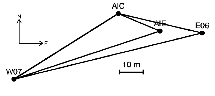
Figure 8: Layout of the baselines for $\nu\,\text{Ophiuchus}$. The longest baseline, E06-W07, contains the zero-crossing.

Figure 9: Coherent integration of the three baselines in the closure triangle separately. It can be seen that the SNR on the W07-E06 baseline is extremely poor.

Figure 10: Coherent integration of the three baselines in the closure triangle. In this case the phase on the long baseline, W07-E06, has been bootstrapped from the two shorter baselines, with the result that the SNR on the baseline is greatly improved.

We will illustrate the use of coherently integrated visibilities by measuring the diameter of a binary star. We make use of measurements of the binary star $\nu\,\text{Ophiuchus}$ on two different days in 2005 and demonstrate how minimally calibrated data can be used to make very high-precision measurements. Table 2 lists the observations. Each observation was performed on five baselines as illustrated in Figure 8. The longest baseline, E06-W07, contains a visibility zero-crossing. This zero-crossing is directly related to the uniform-disk diameter of the star. If we can measure the zero-crossing very accurately we can therefore measure the diameter of the star very precisely. However, we cannot coherently integrate on that baseline directly because the visibility is small and the SNR thus small also. Figure 9 shows the real component of the coherently integrated visibility in that case. Instead we must bootstrap the phase on the long baseline from the measured phase on the two shorter baselines with which it forms a closure triangle. The result is shown in Figure 10 and the SNR is significantly improved.

Figure 11: Plot of the real component (X) of the visibility of all nine observations. The zero-crossing is clearly visible in each observation.

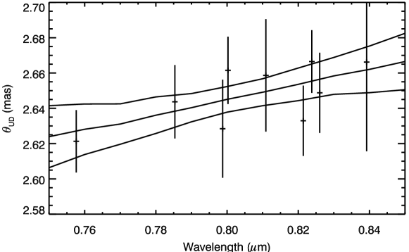
Figure 12: Diameter of the star as a function of wavelength (solid curve) and the uncertainty range out to one standard deviation (dotted curves). At $\lambda=0.80\,\mu\text{m}$ the diameter is determined to better than one part in 350.

We can repeat this procedure for all nine observations and obtain a visibility with good SNR on nice observations of the long baseline. Because the nine observations occur at different hour angle, the projected baseline length will be different. Thus, we expect the zero-crossings to occur at different wavelengths, which we do in-fact see in Figure 11. Measuring the location of the zero-crossing and converting it to a uniform-disk diameter we can then plot these as a function of the wavelength of the visibility zero-crossing, and obtain the star’s diameter as a function of wavelength as illustrated in Figure 12. The produces a remarkable precision of $\theta_{\text{UD}}(0.80\,\mu\text{m})=2.6451\pm 0.0073\,\text{mas}$, or a precision of one part in 364. With only a calibration of the wavelength scale and no amplitude calibration we have thus determined the diameter of a star, from nine observations, to a precision of better than $0.3\%$, and we have also mapped the variation of the diameter with wavelength.

8 Measuring binary stars

Binary stars contain a visibility phase signature in addition to the amplitude signature. It is possible to extract the binary star parameters while considering only the visibility phase. The advantage of using the visibility phase is that it does not suffer from the biases of the visibility amplitude such that the phase often is much more accurate. A separate paper in these proceedings, Jorgensen et al. (2008)[7], discusses the measurements of binaries using coherently integrated visibility phases.

9 Conclusion

In this paper we have outlined the current approach to coherent integration at the NPOI. The meaning of the visibility phase is now well-understood, the visibility amplitudes can be calibrated, and the resulting coherently integrated visibilities can be used to make high-precision scientific measurements, as illustrated by the measurement of the diameter - and it’s variation with wavelength - of $\nu\,\text{Ophiuchus}$.

- [1] J. T. Armstrong, D. Mozurkewich, L. J. Rickard, D. J. Hutter, J. A. Benson, P. F. Bowers, N. M. Elias II, C. A. Hummel, K. J. Johnston, D. F. Buscher, J. H. Clark III, L. Ha, L.-C. Ling, N. M. White, and R. S. Simon, “The Navy Prototype Optical Interferometer,” Astrophys. J. 496, pp. 550–571, 1998.
- [2] A. M. Jorgensen, D. Mozurkewich, J. T. Armstrong, R. Hindsley, T. A. Pauls, G. C. Gilbreath, and S. R. Restaino, “Fringe fitting for coherent integrations with the npoi,” Proc. SPIE 5491, Astronomical Telescopes and Instrumentation , 2004.
- [3] A. M. Jorgensen, D. Mozurkewich, H. Schmitt, T. Armstrong, C. Gilbreath, R. Hindsley, T. A. Pauls, and D. Peterson, “Coherent integrations, fringe modeling, and bootstrapping with the npoi.,” Proc. SPIE 6268, Astronomical Telescopes and Instrumentation , 2006.
- [4] A. M. Jorgensen, D. Mozurkewich, J. T. Armstrong, H. Schmitt, T. A. Pauls, and R. Hindsley, “Improved coherent integration through fringe model fitting,” Astronomical Journal 134, pp. 1544–1550, 2007.
- [5] J. A. Benson, D. Mozurkewich, and S. M. Jefferies, “Active optical fringe tracking at the npoi,” Proc. SPIE 3350, Astronomical Telescopes and Instrumentation , 1998.
- [6] J.-B. L. Bouquin, B. Bauvir, P. Haguenauer, M. Schöller, F. Rantakyrö, and S. Merandi, “First result with AMBER+FINITO on the VLTI: the high-precision angular diameter of V3879 Sagittarii,” A&A 481, pp. 553–557, 2008.
- [7] A. M. Jorgensen, H. Schmitt, R. Hindsley, J. T. Armstrong, T. A. Pauls, D. Mozurkewich, D. J. Hutter, and C. Tycner, “Measurements of binary stars with coherent integration of npoi data,” Proc. SPIE Astronomical Telescopes and Instrumentation (this volume) , 2008.