Luminescence Spectra of Quantum Dots in Microcavities. I. Bosons.

Abstract

We provide a unified theory of luminescence spectra of coupled light-matter systems realized with semiconductor heterostructures in microcavities, encompassing: $i)$ the spontaneous emission case, where the system decays from a prepared (typically pure) initial state, and $ii)$ luminescence in the presence of a continuous, incoherent pump. While the former case has been amply discussed in the literature (albeit mainly for the case of resonance), no consideration has been given to the influence of the incoherent pump. We show how, by provoking a self-consistent quantum state, the pump considerably alters the emission spectra, even at vanishing intensities. The main outcome of our analysis is to unambiguously identify strong-coupling in situations where it appears in disguise or only seems to appear. Here, we consider bosonic matter fields, in which case fully analytical solutions can be obtained. This describes the case of quantum wells or large quantum dots, or the limit of low excitation where the average populations remain much smaller than one.

I Introduction

The dynamics of an optical emitter changes drastically when it is placed in a cavity. The cavity alters the density of states of optical modes, and therefore increases or inhibits interactions with the emitter. The effect was first put to use by Purcell in nuclear magnetic resonance for the practical purpose of thermalizing spins at radio frequencies, by bringing down their relaxation time from $\approx 10^{21}$s to a few minutes Purcell (1946). Kleppner applied the same idea in the opposite way, to increase the relaxation time of an excited atom, i.e., to inhibit its spontaneous emission (SE) Kleppner (1981). The emitter, that in the case of Purcell was sought to be resonant with the cavity mode to increase the photon density of states with respect to the vacuum, was in the case of Kleppner put out of resonance, namely in a photonic gap, where the photon density of states is smaller than in vacuum. This tuning of the relaxation time of an emitter placed in a cavity, now known as the Purcell effect, has many potential technological applications, one of the most compelling being the decrease of the lasing threshold. The effect, that had first been actively looked for with atoms in cavities Goy et al. (1983), was therefore also intensively (and more recently) pursued in the solid state, more prone for massive technological implementations. Semiconductor heterostructures are the state of the art arena for this purpose. They allow to engineer, with an ever rising control, the solid state counterpart of the atomic system to match or isolate their excitation spectra and thus control their behaviour. Typical examples are quantum dots (QDs) placed in cavities made in micropillars, microdisks or photonic crystals, where Purcell inhibition has been distinctly demonstrated Gérard et al. (1998); Kiraz et al. (2002). In this paper, we shall be concerned chiefly with the observed spectra of emission of such an emitter placed in a cavity. In the regime where the effect of the cavity is to lengthen or shorten the lifetime of the excitation, the consequence in the optical spectra is to narrow or broaden the line, respectively.

In the description of the Purcell effect, the possible reabsorption of the photon by the emitter is so weak that it can be neglected. It is responsible for the energy shift known as the Lamb shift, that, in quantum electrodynamics, is interpreted as the perturbative influence of virtual photons emitted and re-absorbed by the emitter. In the case of inhibition of the spontaneous emission, this shift is indeed orders of magnitude smaller than the radiative broadening. In the case where emission is enhanced, and the linewidth narrowed, the probability of reabsorption of a photon by the emitter becomes closer to that of escaping the cavity, until the perturbative—so-called weak-coupling (WC)—regime breaks down and instead strong coupling (SC) takes place. In this case, photons emitted are then reflected by the mirrors and there is a higher probability for their reabsorption by the atom than for their leaking out of the cavity. A whole sequence of absorptions and emissions can therefore take place, known as Rabi oscillations. This regime is of greater interest, as it gives rise to new quantum states of the light-matter coupled system, usually referred to as dressed states in atomic physics and as polaritons in solid-state physics. Experimentally, SC is more difficult to reach, as it requires a fine control of the quantum coupling between the bare modes and in particular to reduce as much as possible all the sources of dissipation. Theoretically, it is better dealt with by first getting rid of the dissipation, and starting with the strong-coupling Hamiltonian ($\hbar$ is taken as 1 along the paper):

$$H=\omega_{a}{a^{\dagger}}a+\omega_{b}{b^{\dagger}}b+g({a^{\dagger}}b+a{b^{\dagger}})$$ (1)

where $a$ and $b$ are the cavity photon and material excitation field operators, respectively, with bare mode energies $\omega_{a}$ and $\omega_{b}$, coupled linearly with strength $g$. The photon operator is a Bose annihilation operator, satisfying the usual commutation rule $[a,{a^{\dagger}}]=1$. Depending on the model for the material excitation, $b$ is described by, typically, another harmonic oscillator (linear model Hopfield (1958)) or a two-level system (Jaynes-Cummings model Jaynes and Cummings (1963)). Those are the most fundamental cases as they describe material fields with Bose and Fermi statistics, respectively. Possible extensions are a collection of harmonic oscillators Rudin and Reinecke (1999) or of two-level systems Dicke (1954), a three-level system Bienert et al. (2004), etc. This paper contains the first part of our work in which we address exclusively the case where $b$ also follows Bose statistics. This is an important case for two reasons. The first one is that in many relevant cases, the matter-field is indeed bosonic, such as the case of quantum wells, or large quantum dots, at low density of excitations. The second reason is that this case provides the limit for vanishing excitations of all the other cases, and is fully solvable analytically. As such, this case provides the backbone for the qualitative understanding of SC. We leave for a further work the case of fermions at larger pumping, more relevant when dealing with small QDs that confine excitations, and more prone to involve genuine quantum mechanics as one quantum of excitation can alter the system’s response. The drawback is that numerical computation is required in this case, and the discussion is therefore of a somehow less fundamental character.

For the rest of the text, it is therefore understood that $b$ is also a Bose operator. For convenience, we shall refer to it as the exciton operator, after the name of a bound electron-hole pair in a semiconductor. Likewise, we shall prefer such terminology as a Quantum Dot (QD) rather than an atom, or polaritons, rather than dressed states, etc. For most purpose, this is semantics only and the results apply in a wide range of systems.

Equation (1) can be straightforwardly diagonalized for bosonic modes, giving $H=\omega_{\mathrm{U}}{p^{\dagger}}p+\omega_{\mathrm{L}}{q^{\dagger}}q$, where

$$\omega_{\begin{subarray}{c}\mathrm{U}\\ \mathrm{L}\end{subarray}}=\frac{\omega_{a}+\omega_{b}}{2}\pm\sqrt{g^{2}+\frac{\Delta^{2}}{4}}\,,$$ (2)

with new Bose operators $p=(\cos\theta)a+(\sin\theta)b$ and $q=-(\sin\theta)a+(\cos\theta)b$, determined by the mixing angle, $\theta=\arctan\big{(}(\frac{\Delta}{2}+\sqrt{g^{2}+\frac{\Delta^{2}}{4}})/g\big{)}$, and the detuning:

$$\Delta=\omega_{a}-\omega_{b}\,.$$ (3)

These new modes are the polaritons (or dressed states) with quantum states $\left|\mathrm{U}\right\rangle={p^{\dagger}}\left|\mathrm{vac}\right\rangle=\cos\theta\left|1,0\right\rangle+\sin\theta\left|0,1\right\rangle$ and $\left|\mathrm{L}\right\rangle={q^{\dagger}}\left|\mathrm{vac}\right\rangle=-\sin\theta\left|1,0\right\rangle+\cos\theta\left|0,1\right\rangle$, where $\left|\mathrm{vac}\right\rangle$ is the vacuum, $\left|1,0\right\rangle$ is the Fock state of one photon and $\left|0,1\right\rangle$ the Fock state of one exciton.

The energies defined by eqn (2) are displayed in Fig. 1 with dashed lines, on top of that of the bare modes, with thick lines, as detuning is varied by changing the energy of the emitter and keeping that of the cavity constant. The anticrossing always keeps the upper mode U higher in energy than the lower L one, strongly admixing the light and matter character of both particles. At resonance, this mixing is maximal:

$$\left|\mathrm{\begin{subarray}{c}\mathrm{U}\\ \mathrm{L}\end{subarray}}\right\rangle=\frac{1}{\sqrt{2}}\left(\left|1,0\right\rangle\pm\left|0,1\right\rangle\right)\,.$$ (4)

If the system is initially prepared as a bare state—which is the natural picture when reaching the SC from the excited state of an emitter—the dynamics is that of an oscillatory transfer of energy between light and matter. In an empty cavity, the time evolution of a state which was an exciton at $t=0$, is given by:

$$\left|\psi(t)\right\rangle =\exp\big{(}-iHt\big{)}\left|0,1\right\rangle\,,$$ (5a)

$$=\sin\theta\cos\theta(e^{-i\omega_{\mathrm{U}}t}-e^{-i\omega_{\mathrm{L}}t})\left|1,0\right\rangle$$

$$+(\sin^{2}\theta e^{-i\omega_{\mathrm{U}}t}+\cos^{2}\theta e^{-i\omega_{\mathrm{L}}t})\left|0,1\right\rangle\,,$$ (5b)

which results in oscillations between the bare modes at the so-called Rabi frequency:

$$\mathcal{R}=\frac{\omega_{\mathrm{U}}-\omega_{\mathrm{L}}}{2}=\sqrt{g^{2}+\frac{\Delta^{2}}{4}}\,.$$ (6)

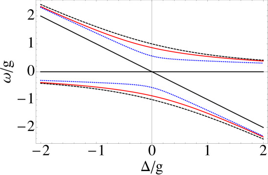
Figure 1: (Color online) Solid black: Bare energies of the cavity photon (horizontal line) and of the exciton (tilted) as a function of detuning $\Delta$. Dashed black: Eigenenergies of the system Hamiltonian, without dissipation nor pumping [eqn (2)]. The exciton-like state at large negative $\Delta$ has become a photon-like state at large positive $\Delta$, and vice-versa. Around $\Delta=0$, both modes are an admixture of exciton and photon. Dotted blue: Correction of the eigenenergies when pump and decay are taken into account for parameters of point (c) in Fig. 9. Solid red: Actual position of the observed peaks in the PL spectra for the same parameters. For these parameters, the three descriptions of SC give the same qualitative results.

The emission spectrum of the system requires dissipation, as it is an obvious practical requisite that the excitation should eventually leak out of the system to be detected from the outside [the energy spectrum of the system is given by eqn (2)]. Dissipation is intrinsic to the bare modes: both the cavity photon and the exciton have a finite lifetime. In presence of dissipation, the system is upgraded from a Hamiltonian description, eqn (1), to a Liouvillian description, with a quantum dissipative master equation for the density matrix $\rho$ defined in the tensor product of the light and matter Hilbert spaces $\mathcal{H}_{a}$ and $\mathcal{H}_{b}$ Carmichael (2002):

$$\partial_{t}\rho=\mathcal{L}_{\gamma}\rho\,.$$ (7)

The Liouvillian $\mathcal{L}_{\gamma}$ still contains the Hamiltonian dynamics of SC, but also takes into account the decays of both the cavity and the emitter, with rates $\gamma_{a}$ and $\gamma_{b}$, respectively:

$$\mathcal{L}_{\gamma}\rho=i[\rho,H]+\sum_{c=a,b}\frac{\gamma_{c}}{2}(2c\rho{c^{\dagger}}-{c^{\dagger}}c\rho-\rho{c^{\dagger}}c)\,,$$ (8)

in which we have considered temperature equal to zero. This equation has been extensively studied Carmichael et al. (1989), although, to the best of our knowledge, not in its most general form. The typical restrictions have been to consider the case of resonance, $\omega_{a}=\omega_{b}$, with only one particular initial condition, namely, the excited state of the emitter in an empty cavity, and to detect the emission of the emitter itself. All together, they describe the spontaneous emission of an emitter placed into a cavity with which it enters into SC. This has been the topical case for decades as this was the case of experimental interest with atoms in cavities.

With the advent of SC in other systems, other configurations start to be of interest. With a QD in a microcavity, the detuning $\Delta$ between the modes, eqn (3), is a crucial experimental parameter, as it can be easily tuned and to a great extent, for instance by applying a magnetic field or changing the temperature. Also in this case, the detection is in the optical mode of the cavity, rather than the direct emission of the exciton emission, because the latter is awkward for various technical reasons of a more or less fundamental character (an example of a fundamental complication is that the emission is enhanced in the cavity mode and suppressed otherwise, and the exciton lifetime is typically much longer, so the exciton emission is much weaker; an example of a petty technical complication is that the exciton detection should be made at an angle and, practically, a lot of samples are grown on the same substrate. Both the substrates and other samples hinder the lateral access to one given sample, whereas all are equally accessible from above). In our system where both modes are bosonic, symmetry allows us to focus on the cavity emission without loss of generality, as we can obtain the leaky excitonic emission by simply exchanging indexes $a,b$ (the spectrum could also have photon-exciton crossed terms that could be computed in a similar way). When we shall turn to the case of a fermionic matter-field, where the exciton emission will become distinctly different and for that reason, important, we shall address exciton emission separately del Valle et al. (2008).

Regarding the initial condition, more general quantum states can now be realized, at least in principle, by coherent control, pulse shaping or similar techniques. Additionally and more importantly, the type of excitation of a cavity-emitter system in a semiconductor is of a different character: the excitation is typically injected by either a continuous wave (cw) laser far above resonance, creating electron-hole pairs that relax incoherently to excite the QD in a continuous flow of excitations, or by electrical pumping as in lasers. This pumping, that is of an incoherent nature typical of semiconductor physics, brings many fundamental changes into the problem that go beyond the mere generalisation of eqn (8). Among the most obvious ones, let us already mention that pure states of the like of eqn (4) do not correspond to the experimental reality. Instead, the system is maintained in a partially mixed state with probabilities $p(n)$ to realize the $n$th excited state. In all cases, a steady state is imposed by the interplay of pumping and decay. The Rabi oscillations of the populations—that is, the coherent exchange of energy between the modes—are always washed out, regardless of the photon-like, exciton-like or polariton-like (eigenstate) character of the density matrix.

In this work, we address both the emission spectra obtained in a configuration of spontaneous emission (SE)—where an initial state is prepared and left to decay, as ruled by eqns (7–8)—under its most general setting, and the case of luminescence emission under the action of a continuous and incoherent pumping that establishes a steady state (SS). We bring all results under a common and unified formalism and show how none of the cases fully encompasses the other. The rest of the paper is organised as follows. In Section II, we present the complete model and we derive and discuss its equation of motion, focusing on the single-time dynamics. In Section III, we obtain fully analytically the main results in both of the cases explicated above, this time focusing more on the two-time dynamics, which Fourier transform gives the luminescence spectra. In Section IV, we discuss the mathematical results derived in the two previous sections, accentuating the physical picture and relying on particular cases for illustration. We consider, in this Section, specifically the case of resonance, where all the concepts manifest more clearly. Finally, in Section V, we give a summary of the main results and provide an index of all the important formulas and key figures of this text. We conclude with a short overview of the continuation of this work that replaces the bosonic emitter with a fermionic one.

II Model

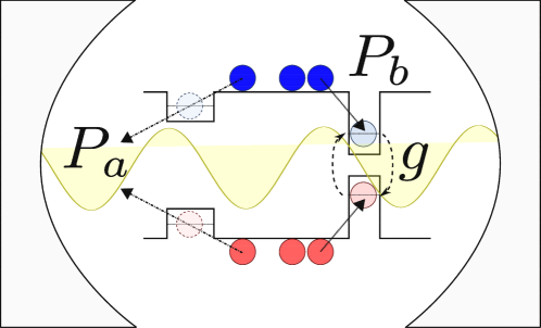
Figure 2: (Color online) Schema of our system for the SS case: self-assembled QDs in a semiconductor microcavity. The QD sketched on the right is in SC with the cavity mode with coupling strength $g$, while the one of the left is in WC. The electron-hole pairs created by the incoherent pumping of the structure provide an effective electronic pumping, $P_{b}$, of the SC dot, while the pumping of the WC dot results in an effective cavity pumping $P_{a}$, through rapid conversion of the excitons into cavity photons.

Our model for the coupling of a QD with a single cavity mode in the presence of incoherent and continuous pumping is sketched in Fig. 2. One QD is strongly coupled to the cavity mode with interaction strength $g$, and is continuously, and incoherently, excited by an electronic pumping $P_{b}$, which, in the microscopic picture, is linked to the rate at which electron-hole pairs relax into the dot. This rate is related in some way to the pumping exerted by the experimentalist. Because of the incoherent nature of this pumping, together with that of the damping, the off-diagonal elements of the QD reduced density matrix (that hold the coherence) are washed out in the SS. We also consider another type of pumping, $P_{a}$, that offers a counterpart for the cavity by injecting photons incoherently at this rate. The major factor to account for such a term is the presence of many other QDs, that have been grown along with the one of interest. Those only interact weakly with the cavity. In most experimental situations so far, it is indeed difficult to find one dot with a sufficient coupling to enter the non-perturbative regime. When this is the case, all the other dots that remain in WC become spectators of the SC physics between the interesting dot and the cavity, and their presence is noticed by weak emission lines in the luminescence spectrum and an increased cavity emission. They are also excited by the electronic pumping that is imposed by the experimentalist, but instead of undergoing SC, they relax their energy into the cavity by Purcell enhancement or inhibition, depending on their proximity with the cavity mode. This, in turn, results in an effective pumping of the cavity Laussy et al. (2008).

To model these two continuous and incoherent pumping, we use Lindblad terms $\mathcal{L}_{\mathrm{P}}$ that substitute the annihilation operator $c$ (standing for $a$ or $b$) by the creation one $c^{\dagger}$, and vice-versa, a procedure which is known to describe pumping terms in a quantum rate equation Rubo et al. (2003). The full Liouvillian now reads (again at zero temperature):

$$\partial_{t}\rho= \mathcal{L}\rho=(\mathcal{L}_{\gamma}+\mathcal{L}_{\mathrm{P}})\rho$$ (9a)

$$= i\omega_{a}[\rho,{a^{\dagger}}a]+i\omega_{b}[\rho,{b^{\dagger}}b]+ig[\rho,{a^{\dagger}}b+a{b^{\dagger}}]$$ (9b)

$$+ \sum_{c=a,b}\frac{\gamma_{c}}{2}(2c\rho{c^{\dagger}}-{c^{\dagger}}c\rho-\rho{c^{\dagger}}c)$$ (9c)

$$+ \sum_{c=a,b}\frac{P_{c}}{2}(2{c^{\dagger}}\rho c-c{c^{\dagger}}\rho-\rho c{c^{\dagger}})\,.$$ (9d)

The microscopic derivation of line (9d) follows from the usual Born-Markov approximation Carmichael (2002). The case of electronic pumping, for instance, is similar to the process of laser gain: the medium requires an inversion of electron-hole population, something that cannot be achieved by means of a simple harmonic oscillator heat bath. The actual process of gaining an exciton in the QD involves the annihilation an electron-hole pair in an external reservoir out of equilibrium (representing either electrical injection or the capture of excitons optically created at frequencies larger than the ones of our system) and the emission of a phonon, that carries the excess of energy, to another one (which can be in thermal equilibrium). A simple effective description of this non-equilibrium process can be made by an inverted harmonic oscillator with levels $E_{p}=-\omega_{\mathrm{P}}(p+1/2)$ maintained at a negative temperature Gardiner (1991). Since the raising operator for the energy decreases the number of quanta of this oscillator, the role of creation and destruction operators is indeed reversed with respect to the usual case of damping.

For the sake of generality, we introduce effective broadenings, that reduce to the decay rates in the SE case but get renormalized by the pumping rate in the SS case:

$$\Gamma_{a,b} =\gamma_{a,b}\,,$$ (SE case) (10a)

$$\Gamma_{a,b} =\gamma_{a,b}-P_{a,b}\,.$$ (SS case) (10b)

We shall also use thoroughly the combinations:

$$\gamma_{\pm}=\frac{\gamma_{a}\pm\gamma_{b}}{4}\quad\text{and}\quad\Gamma_{\pm}=\frac{\Gamma_{a}\pm\Gamma_{b}}{4}\,.$$ (11)

The renormalization of the linewidth in the presence of the pumping term is a bosonic effect. In the case of a single harmonic oscillator driven by pump and decay, the emission spectrum is a Lorentzian lineshape with Full-Width at Half Maximum (FWHM) given by $\gamma-P=P/\langle n\rangle$. The linewidth narrows with the number of particle, in a way reminiscent of the Schallow-Townes effect Scully and Zubairy (2002).

From the relations $\langle O\rangle=\mathrm{Tr}(O\rho)$ and $\partial_{t}\langle O\rangle=\mathrm{Tr}(O\partial_{t}\rho)=\mathrm{Tr}(O\mathcal{L}\rho)$, we can obtain from eqn (9) the single-time mean values of interest for this problem, by solving the equation of motion of the coupled system:

$$\partial_{t}\begin{pmatrix}n_{a}\\ n_{b}\\ n_{ba}\\ n_{ab}\end{pmatrix}=\begin{pmatrix}P_{a}\\ P_{b}\\ 0\\ 0\end{pmatrix}+\begin{pmatrix}-\Gamma_{a}&0&ig&-ig\\ 0&-\Gamma_{b}&-ig&ig\\ ig&-ig&-i\Delta-2\Gamma_{+}&0\\ -ig&ig&0&i\Delta-2\Gamma_{+}\end{pmatrix}\begin{pmatrix}n_{a}\\ n_{b}\\ n_{ba}\\ n_{ab}\end{pmatrix}\,,$$ (12)

where $n_{c}=\langle{c^{\dagger}}c\rangle\in\mathbb{R}$ (for $c=a,b$) and $n_{ab}=\langle{a^{\dagger}}b\rangle=n_{ba}^{*}\in\mathbb{C}$. The SE case corresponds to setting $P_{a,b}=0$ and providing the initial conditions:

$$n_{a}^{0}\equiv n_{a}(0),\quad n_{b}^{0}\equiv n_{b}(0),\quad\text{and}\quad n_{ab}^{0}\equiv n_{ab}(0)\,.$$ (13)

The solutions are heavy, but not devoid of interest. For completeness, and since this is a natural and potentially useful result within the scope of this paper, we provide them in Appendix A.

On the other hand, the SS case corresponds to setting the time derivative on the left hand side of eqn (12) to zero, and solving the resulting set of linear equations. This yields:

$$n_{a}^{\mathrm{SS}} =\frac{g^{2}\Gamma_{+}(P_{a}+P_{b})+P_{a}\Gamma_{b}(\Gamma_{+}^{2}+(\frac{\Delta}{2})^{2})}{4g^{2}\Gamma_{+}^{2}+\Gamma_{a}\Gamma_{b}(\Gamma_{+}^{2}+(\frac{\Delta}{2})^{2})}\,,$$ (14a)

$$n_{b}^{\mathrm{SS}} =\frac{g^{2}\Gamma_{+}(P_{a}+P_{b})+P_{b}\Gamma_{a}(\Gamma_{+}^{2}+(\frac{\Delta}{2})^{2})}{4g^{2}\Gamma_{+}^{2}+\Gamma_{a}\Gamma_{b}(\Gamma_{+}^{2}+(\frac{\Delta}{2})^{2})}\,,$$ (14b)

$$n_{ab}^{\mathrm{SS}} =\frac{\frac{g}{2}(\gamma_{a}P_{b}-\gamma_{b}P_{a})(i\Gamma_{+}-\frac{\Delta}{2})}{4g^{2}\Gamma_{+}^{2}+\Gamma_{a}\Gamma_{b}(\Gamma_{+}^{2}+(\frac{\Delta}{2})^{2})}\,.$$ (14c)

Both photonic and excitonic reduced density matrices are diagonal. They correspond to thermal distributions of particles with the above mean numbers Alicki (1988):

$$\rho^{\mathrm{a}}_{n,p}=\sum_{m}\rho_{n,m;\,p,m}=\delta_{n,p}\frac{(n_{a}^{\mathrm{SS}})^{n}}{(1+n_{a}^{\mathrm{SS}})^{n+1}}\,,$$ (15a)

$$\rho^{\mathrm{b}}_{m,q}=\sum_{n}\rho_{n,m;\,n,q}=\delta_{m,q}\frac{(n_{b}^{\mathrm{SS}})^{m}}{(1+n_{b}^{\mathrm{SS}})^{m+1}}\,.$$ (15b)

Behind their forbidding appearance, eqns (14) enjoy a transparent physical meaning, that they inherit from the semi-classical—and therefore intuitive—picture of rate equations. For instance, when the coupling strength between the two modes, $g$, vanishes, the solutions $n_{a,b}=P_{a,b}/\Gamma_{a,b}$ are those of a source and sink problem for bosons, i.e., of the kind $\partial_{t}n=-\gamma n+P(n+1)$, featuring the famous Bose stimulation effect, whereby the probability of relaxation towards the final state is increased by its population.

III Correlation functions and spectra

We now turn to the main goal of this paper, namely, the luminescence spectrum of the system $s(\omega)$. Physically, it is the intensity (or mean number) of photons in the system with frequency $\omega$, i.e., by definition:

$$s(\omega)=\langle{a^{\dagger}}(\omega)a(\omega)\rangle\,.\\$$ (16)

This is proportional to the intensity of photons emitted by the cavity at this frequency (the direct exciton emission from its recombination is described in a similar way by $\langle{b^{\dagger}}(\omega)b(\omega)\rangle$). It will be more convenient, throughout, to deal with normalized spectra:

$$S(\omega)=s(\omega)\Big{/}\int_{0}^{\infty}\langle{a^{\dagger}}a\rangle(t)dt\,,$$ (17)

so that eqn (17) is now the density of probability that a photon emitted by the system has frequency $\omega$. The Fourier transform of $a(\omega)$ relates the emission spectrum to a two-time correlator through $S(\omega)=\frac{1}{2\pi}\iint_{0}^{\infty}\langle{a^{\dagger}}(t_{1})a(t_{2})\rangle e^{i\omega(t_{2}-t_{1})}dt_{1}dt_{2}/\int\langle{a^{\dagger}}a\rangle(t)dt$, that after a change of variables, can be expressed in terms of the so-called first-order time autocorrelator:

$$G^{(1)}(t,\tau)=\langle{a^{\dagger}}(t)a(t+\tau)\rangle$$ (18)

for positive time delay $\tau=t_{2}-t_{1}>0$. All put together, this yields the usual Fourier-pair relationship between the power spectrum and the autocorrelation function:

$$S(\omega)=\frac{1}{\pi\int_{0}^{\infty}\langle{a^{\dagger}}a\rangle(t)dt}\Re\int_{0}^{\infty}\int_{0}^{\infty}G^{(1)}(t,\tau)e^{i\omega\tau}\,d\tau dt\,.$$ (19)

Equation (19) holds as such in the SE case. In the SS case, care must be taken with cancellation of infinities brought by the ever-increasing time $t$. A technical but straightforward procedure (cf. Appendix B) leads to the expression that explicitly gets rid of the divergences—famously known as the Wiener-Khintchine theorem Mandel and Wolf (1995)—that reads:

$$S^{\mathrm{SS}}(\omega)=\frac{1}{\pi}\frac{1}{n_{a}^{\mathrm{SS}}}\lim_{t\rightarrow\infty}\Re\int_{0}^{\infty}G^{(1)}(t,\tau)e^{i\omega\tau}d\tau\,.$$ (20)

From now on, we shall refer with “SE” and “SS” to the expressions that apply specifically to the spontaneous emission and to the steady state, respectively, leaving free of index those that are of general validity. In some cases, as for instance in eqn (10), no index is required if it is understood that $P_{a/b}$ are defined and equal to zero in the SE case. For that reason, we shall leave $\Gamma$ free of the SE/SS redundant index.

To obtain the spectra of a system whose dynamics is dictated by eqn (9), we therefore need to compute two-time dynamics. This can be done thanks to the quantum regression theorem, according to which, a set of operators $A_{\{\alpha\}}$ that satisfy $\mathrm{Tr}(A_{\{\alpha\}}\mathcal{L}O)=\sum_{\{\beta\}}M_{\{\alpha\beta\}}\mathrm{Tr}(A_{\{\beta\}}O)$ for all $O\in\mathcal{H}_{a}\otimes\mathcal{H}_{b}$ for some $M_{\{\alpha\beta\}}$, yields the equations of motion for the two-time correlators as:

$$\partial_{\tau}\langle O(t)A_{\{\alpha\}}(t+\tau)\rangle=\sum_{\{\beta\}}M_{\{\alpha\beta\}}\langle O(t)A_{\{\alpha\}}(t+\tau)\rangle\,.$$ (21)

In the fully bosonic case, operators $a^{n}b^{m}$ with $\{\alpha\}=(n,m)\in\mathbb{N}$ constitute such a set with $M$ defined by

$$M_{\begin{subarray}{c}nm\\ nm\end{subarray}}=-i(n\omega_{a}+m\omega_{b})-n\frac{\Gamma_{a}}{2}-m\frac{\Gamma_{b}}{2}\,,$$ (22)

$$M_{\begin{subarray}{c}nm\\ n+1,m-1\end{subarray}}=M_{\begin{subarray}{c}mn\\ m-1,n+1\end{subarray}}=-igm\,,$$ (23)

and zero everywhere else. For the computation of the optical spectrum, it is enough to consider $A^{\mu}=a$ and $O={a^{\dagger}}$ in eqn (21). We obtain the equation

$$\partial_{\tau}\mathbf{v}(t,t+\tau)=\mathbf{M}_{1}\mathbf{v}(t,t+\tau)$$ (24)

for the correlators

$$\mathbf{v}(t,t+\tau)=\begin{pmatrix}\langle{a^{\dagger}}(t){a}(t+\tau)\rangle\\ \langle{a^{\dagger}}(t)b(t+\tau)\rangle\end{pmatrix}$$ (25)

where

$$\mathbf{M}_{1}=\begin{pmatrix}M_{\begin{subarray}{c}10\\ 10\end{subarray}}&M_{\begin{subarray}{c}10\\ 01\end{subarray}}\\ M_{\begin{subarray}{c}01\\ 10\end{subarray}}&M_{\begin{subarray}{c}01\\ 01\end{subarray}}\end{pmatrix}=\begin{pmatrix}-i\omega_{a}-\frac{\Gamma_{a}}{2}&-ig\\ -ig&-i\omega_{b}-\frac{\Gamma_{b}}{2}\end{pmatrix}\,.$$ (26)

The formal solution follows straightforwardly from $\mathbf{v}(t,t+\tau)=e^{\mathbf{M}_{1}\tau}\mathbf{v}(t,t)$. Made explicit, it reads (at positive $\tau$):

$$\langle{a^{\dagger}}(t){a}(t+\tau)\rangle=\frac{\exp[-(\Gamma_{+}-i\frac{\Delta}{2})\tau]}{2R}\\ \times\Big{\{}e^{iR\tau}[(R+i\Gamma_{-}-{\Delta}/{2})n_{a}(t)-g\,n_{ab}(t)]\\ {}+e^{-iR\tau}[(R-i\Gamma_{-}+{\Delta}/{2})n_{a}(t)+g\,n_{ab}(t)]\Big{\}}$$ (27)

in terms of the complex Rabi frequency:

$$R=\sqrt{g^{2}-\left(\Gamma_{-}+i\frac{\Delta}{2}\right)^{2}}\,,$$ (28)

that arises as a direct extension of the dissipationless case, eqn (6). For our discussion, it is convenient to decompose $R$ into its real and imaginary parts, $R=R_{\mathrm{r}}+iR_{\mathrm{i}}$. Out of resonance, the Rabi frequency is a complex number with both nonzero real and imaginary parts. On the other hand, at resonance, it is either pure imaginary (in the WC regime), either pure real (in the SC one). For this latter case it is worth defining a new quantity:

$$R_{0}=R(\Delta=0)=\sqrt{g^{2}-\Gamma_{-}^{2}}\,.$$ (29)

In Fig. 3, the real and imaginary parts of $R$ are plotted as a function of $\Gamma_{-}/g$ for various detunings.

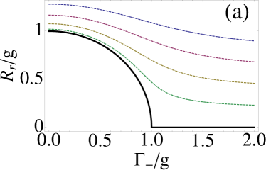
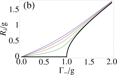
Figure 3: (Color online) Complex Rabi $R/g$, separated in its real (a) and imaginary (b) parts, as a function of the decoherence parameter $\Gamma_{-}/g$ for various detunings ($\Delta/g$ from $-1.6$, up, to 0, bottom, by steps of 0.4). Solid black lines correspond to resonance.

In the limit of high detuning, $|\Delta|\gg g$, regardless of WC or SC, the real part becomes independent of the dissipation (decay and pumping), $R_{\mathrm{r}}\approx|\Delta|/2$, and the imaginary part becomes $R_{\mathrm{i}}\approx\mp\Gamma_{-}$. Therefore, as already pointed out, the limit of bare modes at energies $\omega_{a}=0$ and $\omega_{b}=-\Delta$ broadened with the bare parameters $\Gamma_{a/b}$ (FWHM), is always recovered at large detunings.

Using the result of eqn (27) into the definition of eqn (19), we obtain the formal structure of the emission spectrum:

$$S(\omega)=\frac{1}{2\pi}\Big{[}(\mathcal{L}^{1}+\mathcal{L}^{2})-\Im\{\mathcal{C}\}(\mathcal{L}^{1}-\mathcal{L}^{2})-\Re\{\mathcal{C}\}(\mathcal{A}^{1}-\mathcal{A}^{2})\Big{]}$$ (30)

with $\mathcal{L}(\omega)$ and $\mathcal{A}(\omega)$ some Lorentzian and dispersive functions whose features (position and broadening) are entirely specified by the complex Rabi frequency [eqn (28)], $\Gamma_{+}$ [eqn (11)] and the detuning $\Delta$:

$$\mathcal{L}^{\begin{subarray}{c}1,2\end{subarray}}(\omega)= \frac{{\Gamma_{+}\pm R_{\mathrm{i}}}}{({\Gamma_{+}\pm R_{\mathrm{i}}})^{2}+(\omega-({-\frac{\Delta}{2}\mp R_{\mathrm{r}}}))^{2}}\,,$$ (31a)

$$\mathcal{A}^{\begin{subarray}{c}1,2\end{subarray}}(\omega)= \frac{\omega-({-\frac{\Delta}{2}\mp R_{\mathrm{r}}})}{({\Gamma_{+}\pm R_{\mathrm{i}}})^{2}+(\omega-({-\frac{\Delta}{2}\mp R_{\mathrm{r}}}))^{2}}\,.$$ (31b)

We also introduced $\mathcal{C}$, a complex coefficient given by

$$\mathcal{C} =\frac{\Gamma_{-}+i(\frac{\Delta}{2}+gD)}{R}\,,$$ (32)

that we define in terms of still another parameter, $D$:

$$D=\frac{\displaystyle\int_{0}^{\infty}\langle{a^{\dagger}}b\rangle(t)\,dt}{\displaystyle\int_{0}^{\infty}\langle{a^{\dagger}}a\rangle(t)\,dt}\,.$$ (33)

Written in this form, eqns (30–33) assume a transparent physical meaning with a clear origin for each term. The spectrum consists of two peaks (that we label 1 and 2), as is well known qualitatively for the SC regime. These are composed of a Lorentzian $\mathcal{L}$ and a dispersive $\mathcal{A}$ part. The Lorentzian is the fundamental lineshape for a system with a lifetime, and in the expression above, it inherits most of how the dissipation gets distributed in the coupled system, including the so-called subnatural linewidth averaging that sees the broadening at resonance below the cavity mode width Carmichael et al. (1989). The dispersive part originates from the coupling as in the Lorentz (driven) oscillator. In our system, it stems from the driving of one mode by the other, because of the coupling. This decomposition of each peak in such terms is therefore entirely clear and expected. More quantitatively, the first peak, (e.g.,) is centred at $-\frac{\Delta}{2}-R_{\mathrm{r}}$ and broadened by $\Gamma_{+}+R_{\mathrm{i}}$. As $R_{\mathrm{r}}>0$, this peak corresponds to the lower branch “L”.

So far, all the results hold for both cases of SE and SS. This shows that the qualitative depiction of SC is robust. This made it possible to pursue it in a given experimental system with the parameters of the theoretical models fit for another. This has indeed been the situation with semiconductor results explained in terms of the formalism built for atomic systems.

To be complete, the solution now only requires the boundary conditions that are given by the quantum state of the system. They will affect the parameter $D$, eqn (33), that is therefore the bridging parameter between the two cases. In the next two sections, we address the two cases and their specificities.

III.1 Case of Spontaneous Emission

In the case of Spontaneous Emission Carmichael et al. (1989); Andreani et al. (1999), where the system decays from an initial state, the boundary conditions are supplied for $\tau=0$ by the initial values $\mathbf{v}(t,t)$, i.e., the cavity population, $n_{a}(t)=\langle{a^{\dagger}}a\rangle(t)$ and the coherence element $n_{ab}(t)=\langle{a^{\dagger}}b\rangle(t)$. In turn, those are completely defined by the initial conditions, eqns (13). Although the analytical expression for these mean values as a function of time are cumbersome—see Appendix A—the $D$ coefficient, eqn (33), that determines quantitatively the lineshape, assumes a (relatively) simpler expression:

$$D^{\mathrm{SE}}=\frac{[\frac{g}{2}(\gamma_{a}n^{0}_{b}-\gamma_{b}n^{0}_{a})-2in_{ab}^{0}(\gamma_{+}^{2}-\gamma_{-}^{2})](i\gamma_{+}-\frac{\Delta}{2})+2g^{2}\gamma_{+}\Re n_{ab}^{0}}{g^{2}\gamma_{+}(n_{a}^{0}+n_{b}^{0})+n_{a}^{0}\gamma_{b}(\gamma_{+}^{2}+(\frac{\Delta}{2})^{2}){+g\gamma_{b}(\frac{\Delta}{2}\Re n_{ab}^{0}+\gamma_{+}\Im n_{ab}^{0})}}\,.$$ (34)

To prepare the analogy with the SS case in the next section, we also write the particular case when $n_{ab}^{0}=0$:

$$D^{\mathrm{SE}}=\frac{\frac{g}{2}(\gamma_{a}n^{0}_{b}-\gamma_{b}n^{0}_{a})(i\gamma_{+}-\frac{\Delta}{2})}{g^{2}\gamma_{+}(n_{a}^{0}+n_{b}^{0})+n_{a}^{0}\gamma_{b}(\gamma_{+}^{2}+(\frac{\Delta}{2})^{2})}\,.$$ (35)

This is an important case as it is realized whenever the initial population of one of the modes is zero. Note that in this case, $D^{\mathrm{SE}}$, and therefore also the normalised spectra, do not depend on the magnitude of the populations.

III.2 Case of continuous, incoherent pumping

In the case where the system is excited by a continuous, incoherent pumping, a steady state is reached and the boundary conditions are given by the stationary limit, as time tends to infinity, of the dynamical equation (whose solution is unique). The $D$ parameter, eqn (33), is defined in this case as:

$$D^{\mathrm{SS}}=\frac{n_{ab}^{\mathrm{SS}}}{n_{a}^{\mathrm{SS}}}=\frac{\frac{g}{2}(\gamma_{a}P_{b}-\gamma_{b}P_{a})(i\Gamma_{+}-\frac{\Delta}{2})}{g^{2}\Gamma_{+}(P_{a}+P_{b})+P_{a}\Gamma_{b}(\Gamma_{+}^{2}+(\frac{\Delta}{2})^{2})}\,.$$ (36)

There is a clear analogy between eqn (36)—that corresponds to the SS—and eqn (35)—that corresponds to SE when $n_{ab}^{0}=0$. It is made more meaningful by defining the ratio

$$\alpha =n_{a}^{0}/n_{b}^{0}\qquad(\text{SE case with~{}$n_{ab}^{0}=0$})\,,$$ (37a)

$$\alpha =P_{a}/P_{b}\qquad(\text{SS case})\,,$$ (37b)

in which case eqns (35) and (36) assume the same expression, keeping in mind the definition of eqns (10). Table 1 displays this common expression for $D$ in terms of $\alpha$. The limiting cases when $\alpha\rightarrow 0$ or $\infty$ are also given. They correspond to only photons or excitons as the initial state for the SE, or to the presence of only one kind of incoherent pumping for the SS case.

The analogy and differences between $D^{\mathrm{SE}}$ and $D^{\mathrm{SS}}$ reflect in the spectra $S^{\mathrm{SE}}$ and $S^{\mathrm{SS}}$. For the same $\alpha$, they become identical when the pumping rates are negligible as compared to the decays, $P_{a,b}\ll\gamma_{a,b}$. In this case, where $\Gamma_{\pm,a,b}\approx\gamma_{\pm,a,b}$, the SS system indeed behaves like that of the SE of particles that decay independently and that are, at each emission, either a photon or an exciton, with probabilities in the ratio $\alpha$.

However, in the most general case, $D^{\mathrm{SS}}$ depends on more parameters—namely, $\alpha$ and $\Gamma_{\pm,a,b}$—than $D^{\mathrm{SE}}$, that depends only on $\alpha$ and $\gamma_{\pm,a,b}$, cf. eqn (10). Moreover, the pumping rates $P_{a,b}$ affect $S^{\mathrm{SS}}$ not only through $\alpha$ and $D^{\mathrm{SS}}$, but also in the position and broadening of the peaks (given by $\Gamma_{\pm}$ and $R$). Therefore, the SS is a more general case, from which the SE with $n_{ab}^{0}=0$ can be obtained, but not the other way around. On the other hand, as seen in Table 1, the SS case cannot recover the SE case when $n_{ab}^{0}\neq 0$ (this could be overcome if cross Lindblad pumping terms were introduced in eqn (9) with parameters $P_{ab}$ corresponding to the cross initial mean value $n_{ab}^{0}$, as is done in, e.g., Ref. del Valle et al. (2007), but this describes another system).

In any case, an important fact for the semiconductor community is that a SS with non-vanishing pumping rates is out of reach of the SE of any initial state, which has been the case studied in the literature so far Carmichael et al. (1989); Andreani et al. (1999), and that even in this limiting case, the effective quantum state obtained in the SS should still be resolved self-consistently, rather than assuming for $\alpha$ the particular case $0$ or $\infty$.

$\displaystyle\alpha=\frac{n_{a}^{0}}{n_{b}^{0}}=\frac{P_{a}}{P_{b}}$	$D$
0	$\displaystyle\frac{-\frac{g}{2}(i\Gamma_{+}-\frac{\Delta}{2})\gamma_{b}}{g^{2}\Gamma_{+}+\Gamma_{b}(\Gamma_{+}^{2}+(\frac{\Delta}{2})^{2}))}$
$0<\alpha<\infty$	$\displaystyle\frac{\frac{g}{2}(i\Gamma_{+}-\frac{\Delta}{2})(\gamma_{a}-\gamma_{b}\alpha)}{g^{2}\Gamma_{+}(1+\alpha)+\alpha\Gamma_{b}(\Gamma_{+}^{2}+(\frac{\Delta}{2})^{2}))}$
$\infty$	$\displaystyle\frac{(i\Gamma_{+}-\frac{\Delta}{2})\gamma_{a}}{2g\Gamma_{+}}$

Table 1: Expression of $D$, eqn (33), as a function of $\alpha$, eqns (37), in the SE (with $\Gamma_{\pm,a,b}\rightarrow\gamma_{\pm,a,b}$ and $n_{ab}^{0}=0$) and SS cases. $D$ embodies in the luminescence spectrum the influence of the quantum state of the system. The latter is specified by the initial condition in SE, or the pumping/decay interplay in the SS.

III.3 Discussion

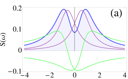
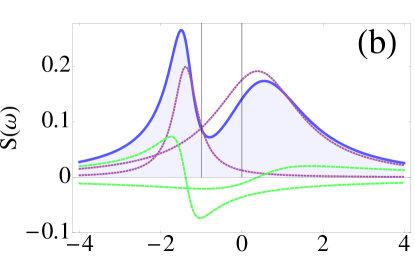
Figure 4: (Color online) Strong-coupling SS spectra (blue solid line) and their decomposition into Lorentzian (dotted purple) and dispersive parts (dashed green) for various detunings ($\Delta/g=0,1,3$) with parameters of point (c) of Fig. 9: $\gamma_{a}=3.8g$, $\gamma_{b}=0.1g$, $P_{a}=0.5g$, $P_{b}=0.1g$. The vertical black lines mark the positions of the bare modes, showing the “level repulsion” of SC.

With this exposition of the analytical expressions of the luminescence spectra, and the discussion of their similarity and distinctions that we have just given, the coverage of the problem is complete and comprehensive. In order to give a more physical picture of these abstract results, we shall in the rest of this paper illustrate the implications that this bears in practical terms. We consider the case of resonance for this purpose, for reasons detailed in the next section. This will also allow us to provide self-contained expressions for the spectra, that can be used more conveniently to plot the expression or use the model in a nonlinear fitting of the experimental data Reithmaier et al. (2004); Yoshie et al. (2004); Peter et al. (2005). The system lends itself naturally to a global fitting, i.e., constraining all fitting parameters over the various detuning cases, where only the detuning is allowed to vary, while optimising them globally Laussy et al. (2008). There is no difficulty in extending all the discussions that follow to arbitrary detunings. For instance, Fig. 4 shows the SS spectra and their mathematical decompositions into Lorentzian and dispersive parts, as detuning is varied. Figs. (b) and (c) are obtained using eqn (30–33), and in this particular case, the expression (36) for $D$. Fig. (a), the case at resonance, can be obtained in the same way, but in next Section we shall bring all these results together in a condensed expression [eqn (49)].

More importantly, as we shall soon appreciate, the resonant case is the pillar of the SC physics. The main output of the out-of-resonance case is to help identify or to characterise the resonance, for instance by localising it in an anticrossing or by providing useful additional constrains with only one more free parameter in a global fitting. Even a slight detuning brings features of WC into the SC system and ultimately, when $\Delta\gg g$, the complex Rabi frequency converges into the same expression for both regimes (as showed in Fig. 3). This is why we now consider the SC problem in its purest form: when the coupling between the modes is optimum.

IV Strong & Weak Coupling at resonance

Strong-coupling is most marked at resonance, and this is where its signature is experimentally ascertained, in the form of an anticrossing. Fundamentally, there is another reason why resonance stands out as predominant: this is where a criterion for SC can be defined unambiguously in presence of dissipation:

WC and SC are formally defined as the regime where the complex Rabi frequency at resonance, eqn (29), is pure imaginary (WC) or real (SC).

This definition, that takes into account dissipation and pumping, generalises the classification found in the literature, and is one of the main results of this work. The reason for this definition is mainly to be found in the behaviour of the time autocorrelator, eqn (27), that is respectively damped or oscillatory as a result. The exponential damping is the usual manifestation of dissipation, that decays the correlations in the field, even when a steady state is maintained. On the other hand, in the same situation of steady averages (no dynamics) but now in SC, the oscillations with $\tau$ are the mark of a coherent exchange between the bare fields (the photon field and exciton field).

Figure 5: (Color online) Time dynamics of the correlator $\Re\langle{a^{\dagger}}(t){a}(t+\tau)\rangle^{\mathrm{SE}}$, cf. eqn (27). Only the pattern of oscillations is of interest here (lighter blues correspond to higher values). In all cases, both the $t$ and $\tau$ dynamics tend to zero. Figures (a) and (b) show the SE of an exciton and of an upper polariton, respectively, in a very strongly-coupled system ($\gamma_{a}=0.2g$ and $\gamma_{b}=0.1g$). Fig. (c) shows the SE of an exciton in weak-coupling ($\gamma_{a}=5.9g$). The oscillations in $\tau$, rather than in $t$, are the mark of SC.

In the literature, one sometimes encounters the confusion that SC is linked to a periodic transfer of energy or of population between the photon and exciton field, or that it follows from a chain of emissions and absorptions. This is an incorrect general association as one can explicit cases with apparent oscillations of populations that correspond to weak coupling, or on the contrary, cases with no oscillations of populations that are in strong coupling. The two concepts are therefore not equivalent, as none implies the other. This is illustrated for the SE case in Figs. 5a, 5b and 6 on the one hand, where the system is in SC, and in Fig. 5c and 7 on the other hand, where it is in WC. In SS, there is no $t$ dynamics in any case, so oscillations of populations are clearly unrelated to weak or strong coupling. In SE, the distinction is clearly seen in Fig. 5 where both the $t$ and $\tau$ dynamics are shown in a contour-plot in the case where the system is initially prepared as an exciton, (a) and (c), or as a polariton, (b). In the polariton case, the dynamics in $t$ is simply decaying (because of the lifetime), while it is clearly oscillating in $\tau$, were the proper manifestation of SC is to be found. The $t$ decay is not exactly exponential because in the presence of dissipation, the polariton is not anymore an ideal eigenstate (the larger the dissipation, the more the departure). However this effect in SC is so small that it only consists in a small “wobbling” of the $\tau$ contour lines. On the other hand, the exciton, (a), that is not an eigenstate, features oscillations both in the $t$ dynamics (the one often but unduly regarded as the signature of SC), as well as the $\tau$ dynamics. In stark contrast, the exciton in WC, (c), bounces with $t$. This, that might appear as an oscillation, is not, as it happens only once and is damped in the long-time values. This behaviour is shown quantitatively in Fig. 6 for SC and Fig. 7 for WC, where the population $n_{a}(t)$ is displayed for the SE of an exciton (blue solid), a photon (purple dashed) and an upper polariton (brown dotted), respectively, along with the luminescence spectrum that they produce (detected in the cavity emission). Here it is better seen how, for instance, the polariton-decay is wobbling as a result of the dissipation, that perturbs its eigenstate-character and leaks some population to the lower polariton. More importantly, note how very different the spectra are, depending on whether the initial state is a photon or an exciton, despite the fact that the dynamics is similar in both cases (see the inset in log-scale of their respective populations). The PL spectrum observed in the cavity emission is much better resolved when the system is initially in a photon state, than it is when the system is initially in an exciton state. The splitting is larger and the overlap of the peaks smaller in the former case. This will find an important counterpart in the SS case. In Fig. 7, the corresponding case of WC is shown for clarity, with a decay of populations and possible oscillations.

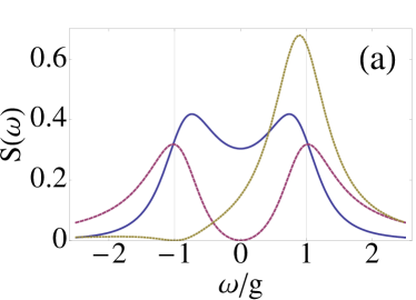
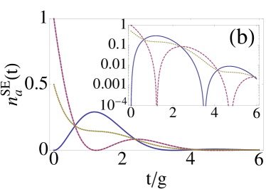
Figure 6: (Color online) Strong-Coupling spectra $S_{0}^{\mathrm{SE}}(\omega)$ (left) and its corresponding mean number dynamics $n_{a}^{\mathrm{SE}}(t)$ (right) for the SE of three different initial states: In blue solid, one exciton; in purple dashed, one photon and in brown dotted, one upper polariton. Parameters are $\gamma_{a}=1.9g$ and $\gamma_{b}=0.1g$. Inset of (b) is the same in log-scale.

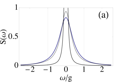
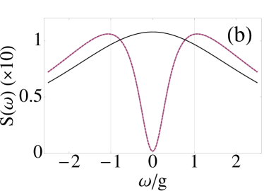
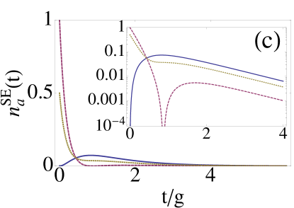
Figure 7: (Color online) Weak-Coupling spectra $S_{0}^{\mathrm{SE}}(\omega)$ (upper) and its corresponding mean number dynamics $n_{a}^{\mathrm{SE}}(t)$ (lower) for the SE of an exciton (a) and a photon (b) as the initial condition. In all figures, solid blue corresponds to the decay of an exciton; dashed purple to the decay of a photon and dotted brown to the decay of an upper polariton. For comparison, we plotted in (a) and (b), with solid black lines, the very different bare emission ($g=0$) of an exciton and photon respectively. Also in (a), in dashed black, that of an exciton decaying with the Purcell rate $\gamma_{\mathrm{P}}=4g^{2}/\gamma_{a}$. Parameters are $\gamma_{a}=1.9g$ and $\gamma_{b}=0.1g$. Inset of (c) is the same in log-scale.

Figure 8 shows the $\tau$ dynamics in the SS (when the $t$ dynamics has converged and is steady), for five cases of interest to be discussed later (in Fig. 9). A first look at the dynamics would seem to gather together a group of two curves that decay exponentially to good approximation (and remain positive as a result), and another group of three that assume a local minimum. The correct classification is the most counter-intuitive in this regard, as it puts together the dashed lines on the one hand and the solid on the other, i.e., scrambling them together. The mathematical reason for this classification is revealed in the inset, where the same dynamics is plotted on log-scale. The dashed (resp. solid) lines correspond to parameters where the system is in WC (resp. SC) according to our definition, i.e., to values of $R$ that are imaginary on the one hand and real on the other. In log-scale, this corresponds respectively to a damping of the correlator, against oscillations with an infinite number of local minima. Note that the blue dashed line features one local minimum, which does not correspond to an oscillatory—or coherent-exchange—behaviour of the fields, but rather to a jolt in the damping. These considerations that may appear abstract at this level will later turn out to show up as the actual emergence of splitted (dressed) states or not in the emitted spectrum.

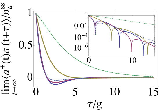
Figure 8: (Color online) Dynamics of $\lim_{t\rightarrow\infty}\langle{a^{\dagger}}(t){a}(t+\tau)\rangle/n_{a}^{\mathrm{SS}}$, eqn (27) and (14a), for the SS corresponding to the points (a)–(e) in Fig. 9. In inset, the same in log-scale. Solid lines (b, blue; c, purple and d, brown) of SC feature oscillations of the correlator, as the mark of SC. Dashed lines (a, green and e, blue) correspond to WC. Note that although the blue dashed line (e) appears to be similar to other SC lines, it does not oscillate in the log-scale, where it only features a single local minimum. In the same way, the brown line (d) that seems not to oscillate actually features an infinite set of local minima, as is revealed in the log scale.

We now return to the general (SE/SS) expression for the spectra, eqn (30), that, at resonance in SC, simplifies to:

$$S_{0}(\omega)=\frac{1}{2\pi}\Bigg{[}(\mathcal{L}_{\mathrm{s}}^{1}+\mathcal{L}_{\mathrm{s}}^{2})-\frac{g\Re\{D_{0}\}}{R_{0}}(\mathcal{L}_{\mathrm{s}}^{1}-\mathcal{L}_{\mathrm{s}}^{2})\\ +\frac{g\Im\{D_{0}\}-\Gamma_{-}}{R_{0}}(\mathcal{A}_{\mathrm{s}}^{1}-\mathcal{A}_{\mathrm{s}}^{1})\Bigg{]}$$ (38)

where we used the definition for the Rabi frequency at resonance, eqn (29), and

$$\mathcal{L}_{\mathrm{s}}^{\begin{subarray}{c}1,2\end{subarray}}(\omega)= \frac{\Gamma_{+}}{\Gamma_{+}^{2}+(\omega\pm R_{0})^{2}}\,,$$ (39a)

$$\mathcal{A}_{\mathrm{s}}^{\begin{subarray}{c}1,2\end{subarray}}(\omega)= \frac{\omega\pm R_{0}}{\Gamma_{+}^{2}+(\omega\pm R_{0})^{2}}\,.$$ (39b)

In the weak coupling regime, with $R_{0}$ pure imaginary ($g<|\Gamma_{-}|$), the positions of the two peaks collapse onto the centre, $\omega_{a}=\omega_{b}=0$. Defining $iR_{\mathrm{w}}=R_{0}$, with $R_{\mathrm{w}}=\sqrt{\Gamma_{-}^{2}-g^{2}}$ a real number, the general expression for the spectra rewrites as:

$$S_{0}^{\mathrm{w}}(\omega) =\frac{1}{2\pi}\left(1+\frac{\Gamma_{-}-g\Im\{D_{0}\}}{R_{\mathrm{w}}}\right)\mathcal{L}_{\mathrm{w}}^{1}$$

$$+\frac{1}{2\pi}\left(1-\frac{\Gamma_{-}-g\Im\{D_{0}\}}{R_{\mathrm{w}}}\right)\mathcal{L}_{\mathrm{w}}^{2}$$

$$-\frac{1}{2\pi}\frac{g\Re\{D_{0}\}}{R_{\mathrm{w}}}(\mathcal{A}_{\mathrm{w}}^{1}-\mathcal{A}_{\mathrm{w}}^{2})\,,$$ (40)

with the Lorentzian and dispersive contributions now given by:

$$\mathcal{L}_{\mathrm{w}}^{\begin{subarray}{c}1,2\end{subarray}}(\omega)= \frac{{\Gamma_{+}\pm R_{\mathrm{w}}}}{({\Gamma_{+}\pm R_{\mathrm{w}}})^{2}+\omega^{2}}$$ (41a)

$$\mathcal{A}_{\mathrm{w}}^{\begin{subarray}{c}1,2\end{subarray}}(\omega)= \frac{\omega}{(\Gamma_{+}\pm R_{\mathrm{w}})^{2}+\omega^{2}}\,.$$ (41b)

We now address the specifics of the SE and SS cases.

IV.1 Case of Spontaneous Emission

In the most general case of SE, the $D^{\mathrm{SE}}$ coefficient at resonance, $D_{0}^{\mathrm{SE}}$, is a complex number. If the initial condition further fulfils $\Re n_{ab}^{0}=0$, it becomes pure imaginary. Usually, the initial states considered are independent states of photons or excitons (not a quantum superposition), where indeed $n_{ab}^{0}=0$ Carmichael et al. (1989); Andreani et al. (1999). In these cases,

$$D_{0}^{\mathrm{SE}}=i\frac{\frac{g}{2}(\gamma_{a}n^{0}_{b}-\gamma_{b}n^{0}_{a})}{g^{2}(n_{a}^{0}+n_{b}^{0})+n_{a}^{0}\gamma_{b}\gamma_{+}}\,,$$ (42)

which yields the following expression for the spectrum:

$$S_{0}^{\mathrm{SE}}(\omega)=\frac{1}{\pi}\frac{\frac{\gamma_{a}+\gamma_{b}}{2}(g^{2}+\frac{\gamma_{a}\gamma_{b}}{4})(g^{2}n_{b}^{0}+\frac{n_{a}^{0}\gamma_{b}^{2}}{4}+n_{a}^{0})}{\left(\omega^{4}+\omega^{2}(\frac{\gamma_{a}^{2}+\gamma_{b}^{2}}{4}-2g^{2})+(g^{2}+\frac{\gamma_{a}\gamma_{b}}{4})^{2}\right)\left(g^{2}(n_{a}^{0}+n_{b}^{0})+n_{a}^{0}\gamma_{b}\frac{\gamma_{a}+\gamma_{b}}{4}\right)}\,.$$ (43)

As noted earlier, the SE spectrum of exciton observed in the leaky modes is obtained from eqn (43) by exchanging the indices $a\leftrightarrow b$. We illustrate this with the two particular cases that follow.

The typical detection geometry for the spontaneous emission of an atom in a cavity consists in having the atom in its excited state as the initial condition, and observing its direct emission spectrum. In this case the role of the cavity is merely to affect the dynamics of its relaxation, that is oscillatory with the light-field in the case of SC. This case corresponds to $n^{0}_{b}=1$ and $n^{0}_{a}=n^{0}_{ab}=0$ in eqn (43) with $a\leftrightarrow b$. This gives Carmichael et al. (1989):

$$S_{0}^{\mathrm{SE}}(\omega)=\frac{1}{\pi}\frac{\frac{\gamma_{a}+\gamma_{b}}{2}(g^{2}+\frac{\gamma_{a}\gamma_{b}}{4})(\frac{\gamma_{a}^{2}}{4}+\omega^{2})}{\omega^{4}+\omega^{2}(\frac{\gamma_{a}^{2}+\gamma_{b}^{2}}{4}-2g^{2})+(g^{2}+\gamma_{a}\frac{\gamma_{a}+\gamma_{b}}{4})(g^{2}+\frac{\gamma_{a}\gamma_{b}}{4})^{2}}\,.$$ (44)

In the semiconductor case, one would typically still have in mind the excited state of the exciton as the initial condition, but this time, this is the cavity emission that is probed. The initial condition is therefore the same as before but without interchanging $a$ and $b$ in eqn (43), which reads in this case:

$$S_{0}^{\mathrm{SE}}(\omega)=\frac{1}{\pi}\frac{2(\gamma_{a}+\gamma_{b})(4g^{2}+\gamma_{a}\gamma_{b})}{16\omega^{4}-4\omega^{2}(8g^{2}-\gamma_{a}^{2}-\gamma_{b}^{2})+(4g^{2}+\gamma_{a}\gamma_{b})^{2}}\,.$$ (45)

The difference in the lineshape due to the initial quantum state is seen in Fig. 6. The visibility of the line-splitting is much reduced in the case of an exciton in SC which SE is detected through the cavity emission, than in the case of a photon. With a polariton as an initial state, only one line is produced.

Again, by reason of symmetry, interchanging $a\leftrightarrow b$ in eqns (44) and (45), correspond to the SE of the system prepared as a photon at the initial time and detected in, respectively, the cavity emission on the one hand (eqn 44, $a\leftrightarrow b$), and in the leaky mode emission on the other hand (eqn 45). In the latter case, the spectrum is invariant under the exchange $a\leftrightarrow b$. Fig. (6) also hints to the changes brought by the detection channel (direct emission of the exciton or through the cavity mode).

If $n^{0}_{a}=0$ or $n^{0}_{b}=0$ (in which case $n^{0}_{ab}=0$), the normalized spectra do not depend on the nonzero value $n_{b}^{0}$ or $n_{a}^{0}$. That is, one cannot distinguish in the lineshape, the decay of one exciton from that of two, or more. In the more general case, when $n_{ab}^{0}\neq 0$, the peaks can be differently weighted. For instance, starting with an upper polariton $|\phi_{0}\rangle=(|1,0\rangle+|0,1\rangle)/\sqrt{2}$ ($n_{a}^{0}=n_{b}^{0}=n_{ab}^{0}=1/2$) gives rise to a dominant upper-polariton peak (labelled 2 in the above equations, as seen in the brown dotted line in Fig. 6). One can classify the possible lineshapes obtained for various initial states. For instance, as we have just mentioned, the normalized spectrum of $\left|0,n\right\rangle$ as an initial state, is the same whatever the nonzero $n$, which is not entirely unexpected from a linear model. From the previous statement, the same spectrum is also obtained for a coherent state or a thermal state of photons, or indeed any quantum state, as long as the exciton population remains zero. In the same way, the PL spectrum of the product of coherent states in the photon and exciton fields, $\left|z\right\rangle\left|z^{\prime}\right\rangle$ with $z=z^{\prime}\in\mathbb{C}^{*}$, is the same as that of a polariton state $\left|0,1\right\rangle+\left|1,0\right\rangle$, although both are very different in character: a classical state on the one hand and a maximally entangled quantum state on the other.

IV.2 Case of continuous, incoherent pumping

In the SS, at resonance, $D_{0}^{\mathrm{SS}}$ is pure imaginary:

$$D_{0}^{\mathrm{SS}}=i\frac{\frac{g}{2}(\gamma_{a}P_{b}-\gamma_{b}P_{a})}{g^{2}(P_{a}+P_{b})+P_{a}\Gamma_{b}\Gamma_{+}}\,,$$ (46)

and the term that consists in the difference of Lorentzians in eqn (30) disappears: $\Im\{\mathcal{C}\}=0$. As a result, the two peaks are equally weighted for any combination of parameters:

$$S_{0}^{\mathrm{SS}}(\omega)= \frac{1}{2\pi}\Bigg{[}(\mathcal{L}_{\mathrm{s}}^{1}+\mathcal{L}_{\mathrm{s}}^{2})+\frac{g\Im\{D_{0}^{\mathrm{SS}}\}-\Gamma_{-}}{R_{0}}(\mathcal{A}_{\mathrm{s}}^{1}-\mathcal{A}_{\mathrm{s}}^{2})\Bigg{]}\,.$$ (47)

The only way to weight more one of the peaks than the other in the SS of an incoherent pumping, would be to pump directly the polariton (dressed) states, as is the case in higher-dimensional systems were polaritons states with nonzero momentum relax into the ground state Laussy et al. (2004) or in 0D case when cross pumping is considered del Valle et al. (2007). In our present model, however, such terms are excluded. The two peaks of the Rabi doublet, composed of a Lorentzian and a dispersive part, are both symmetric with respect to $\omega_{a}=\omega_{b}=0$. Only if $\Im\{D_{0}^{\mathrm{SS}}\}=\Gamma_{-}/g$, the spectrum of eqn (47) consists exclusively of two Lorentzians. The parameters that correspond to this case are those fulfilling either $g^{2}=\frac{P_{a}}{P_{b}-P_{a}}\Gamma_{b}\Gamma_{-}$ or $\Gamma_{+}=0$. The second case corresponds to the limiting case of diverging populations, where the SC becomes arbitrarily good. In the most general case, the dispersive part will contribute to the fine quantitative structure of the spectrum, bringing closer or further apart the maxima and thus altering the apparent magnitude of the Rabi splitting. In some extreme cases, as we shall discuss, it even contrives to blur the resolution of the two peaks and a single peak results, even though the modes split in energy. As for the weak coupling formula, it simplifies to:

$$S_{0}^{\mathrm{w}}(\omega) =\frac{1}{2\pi}\left(1+\frac{\Gamma_{-}-g\Im\{D_{0}\}}{R_{\mathrm{w}}}\right)\mathcal{L}_{\mathrm{w}}^{1}$$

$$+\frac{1}{2\pi}\left(1-\frac{\Gamma_{-}-g\Im\{D_{0}\}}{R_{\mathrm{w}}}\right)\mathcal{L}_{\mathrm{w}}^{2}\,.$$ (48)

Both decompositions, eqns (47) and (IV.2), have been given to spell-out the structure of the spectra in both regimes. The unified expression that covers them both reads explicitly:

$$S_{0}^{\mathrm{SS}}(\omega)=\frac{1}{\pi n_{a}^{\mathrm{SS}}}\frac{8g^{2}P_{b}+2P_{a}(4\omega^{2}+\Gamma_{b}^{2})}{16\omega^{4}-4\omega^{2}(8g^{2}-\Gamma_{a}^{2}-\Gamma_{b}^{2})+(4g^{2}+\Gamma_{a}\Gamma_{b})^{2}}\,.$$ (49)

It is the counterpart for SS of eqn (43), for SE. The case of excitonic emission can also be obtained, as for SE, by interchanging the indices $a\leftrightarrow b$.

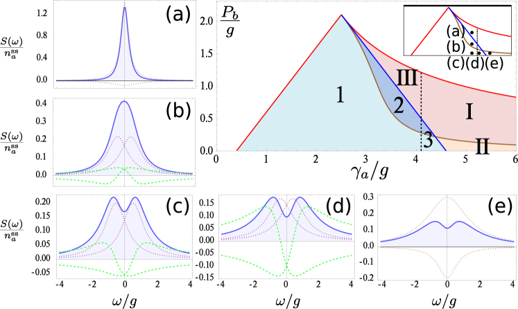
Figure 9: (Color online) Phase space of the SS Strong/Weak Coupling as a function of $P_{b}/g$ and $\gamma_{a}/g$ for the parameters $\gamma_{b}=0.1g$ and $P_{a}/g=0.5g$. The red lines, eqns (52–53), delimit the region where there is a steady state. The blue line, eqn (54), separates the strong (in shades of blue) from the weak (shades of red) coupling regions. The dotted black line, $\gamma_{a}=4g+\gamma_{b}$, separates SC and WC regions in the absence of pumping. The brown line, eqn (56), separates the regions where one (dark blue) or two (light blue) peaks can be resolved in the luminescence spectra. This delineates three areas in the SC region: (1) two peaks are resolved in the spectra, (2) the two peaks cannot be resolved and effectively merge into one, albeit in SC, and (3) SC is achieved thanks to the pump $P_{a}$ (with one or two peaks visible depending of the overlap with the light or dark area) despite the large dissipation that predicts WC according to eqn (50). In the same way we can distinguish three regions in weak coupling: (I) standard WC, (II) SC with a two peaked spectrum and (III) WC due to pumping $P_{b}$. The surrounding figures (a) to (e) show spectra from these regions and their decomposition into, Lorentzian and dispersive parts in SC, or Lorentzians centred at zero in the WC. Parameters correspond to the points in the inset: (a) $\gamma_{a}=3.8g$ and $P_{b}=g$, (b) $\gamma_{a}=3.8g$ and $P_{b}=0.5g$, (c) $\gamma_{a}=3.8g$ and $P_{b}=0.1g$, (d) $\gamma_{a}=4.2g$ and $P_{b}=0.1g$, (e) $\gamma_{a}=4.8g$ and $P_{b}=0.1g$. Observe how, in SC, two eigenstates have emerged in purple dotted lines, even in the cases—like in (b)—where they are not seen in the total spectrum. In the same way, in WC, all the emission emanates from the origin, although a two-peak structure can arise as a result of a resonance, also centred at the origin.

IV.3 Discussion

Although the spectra in the semiconductor case that are probed at negligible electronic pumping ($P_{b}\ll 1$) with no cavity pumping at all ($P_{a}=0$), are in principle described by the same expression as that of the SE case used in the atomic model, in practise, however, both of these conditions can be easily violated. The renormalization of $\gamma_{b}$ with $P_{b}$ brings significant corrections well into the linear regime. For instance, for parameters of point (c) in Fig. 9 with $P_{a}=0$, the rate $P_{b}$ that is needed to bring a $100\%$ correction to $\gamma_{b}$ yields, according to eqns (14a) and (14b), averages much below unity, namely, $n_{a}^{\mathrm{SS}}\approx 0.026$ and $n_{b}^{\mathrm{SS}}\approx 0.121$. By the time $n_{b}$ reaches unity, with $n_{a}$ still one fourth smaller, the correction on the effective decay rate has became 400%. As this is $n_{a}$ which is proportional to the signal detected in the laboratory, the electronic pumping must be kept very small so that corrections to the effective linewidth can be safely neglected. As the more interesting nonlinear regime is probed, the renormalized $\Gamma$s become very different from the bare $\gamma$s.

Second, even in the vanishing electronic pumping limit, it must be held true that $P_{a}$ is zero. Even if only an electronic pumping is supplied externally by the experiment, the pumping rates of the model are the effective excitation rates of the cavity and exciton field inside the cavity, and it is clear that photons get injected in the cavity in structures that consists of numerous spectator dots surrounding the one in SC (cf. Fig. 2). Although most of these dots are in WC with the cavity, they affect the dynamics of the SC QD by pouring cavity photons in the system. In the steady state, following our previous discussion, this corresponds to changing the effective quantum state for the emission of the strongly-coupled QD. As we shall see in more detail in what follows, this bears huge consequences on the appearance of the emitted doublet, especially on its visibility.

To fully appreciate the importance and deep consequences of these two provisions made by the SS case on its SE counterpart, we devote the rest of this Section to a vivid representation in the space of pumping and decay rates parameters. Now that it has been made clear what is the relationship of the SE case with respect to the SS one, we shall focus on the latter that is the adequate, general formalism to describe SC of QDs in microcavities.

In presence of a continuous, incoherent pumping, the criterion for strong-coupling—from the requirement of energy splitting and oscillations in the $\tau$ dynamics that we have discussed above—gets upgraded from its usual expression Carmichael et al. (1989):

$$g>|\gamma_{-}|\,,$$ (50)

to the more general condition:

$$g>|\Gamma_{-}|\,.$$ (51)

The quantitative and qualitative implications and their extent are shown in Fig. 9, where we have fixed the parameters $\gamma_{b}=0.1g$ and $P_{a}/g=0.5g$, and outlined the various regions of interest as $P_{b}$ and $\gamma_{a}$ are varied. This choice of representation allows us to investigate the changes that can be easily imprinted experimentally in the system: by tuning $P_{b}$ on a system of varying quality with regard to SC, as specified by its quality factor that tunes $\gamma_{a}$.

The red lines, that enclose the filled regions, delimit a frontier above which the pump is so high that populations diverge (there is no steady state). This is expressed mathematically by the condition that the common denominator of the mean values in eqns (14) vanishes. It is equivalent to setting the total decay rate of the system—that should remain positive in order for the correlators to decay in time—to zero. In the SC regime, such a rate is given by $\Gamma_{+}$ and therefore the condition for a SS reads:

$$P_{b}=\gamma_{a}+\gamma_{b}-P_{a}\,,\quad(\mathrm{i.e.,~{}}\Gamma_{+}=0)\,.$$ (52)

In the WC regime, the system decays with an effective Purcell rate and the condition transforms into

$$P_{b}=\frac{4g^{2}}{\gamma_{a}+\gamma_{b}-P_{a}}\,.$$ (53)

The main separation inside that region where a SS exists, is that between SC (in shades of blue, inside the triangle) and WC (in shades of red, on its right elbow). The blue solid line that marks this boundary, specified by

$$P_{a}=4g-\gamma_{a}+\gamma_{b}+P_{a}\,,\quad(\mathrm{i.e.,~{}}g=|\Gamma_{-}|)\,,$$ (54)

separates the weak and strong coupling regions. The dashed vertical black line, specified by

$$\gamma_{a}=4g+\gamma_{b}\,,\quad(\mathrm{i.e.,~{}}g=|\gamma_{-}|)\,,$$ (55)

corresponds to the standard criterion of SC (without incoherent pumping).

The light-blue region, labelled 1 on Fig. 9, corresponds to SC as it is generally understood. It has a clear splitting of the lines in the luminescence spectrum. The dark-blue region, labelled 2, corresponds to SC, according to the requisite that $R_{0}$ be real, but with a broadening of the lines so large that in the luminescence spectrum, eqn (47), only one peak is resolved. This region is delimited by the brown line, which is the solution of the equation $d^{2}S(\omega)/d\omega^{2}|_{\omega=0}=0$, i.e., with no concavity at the origin. From this condition follows the implicit equation:

$$(3\Gamma_{+}-\Gamma_{-})g^{2}+(\Gamma_{-}-\Gamma_{+})^{3}+g|D_{0}|(g^{2}-\Gamma_{-}^{2}+3\Gamma_{+}^{2})=0$$ (56)

that yields two solutions, only one of which is physical (the other is placed on the red line $\Gamma_{+}=0$, where the system diverges). Note that this line extends into the WC region, as we shall discuss promptly. The distinction between line-splitting as it results from the emergence of new dressed states in the SC, and the observation of two peaks in the spectrum, is seen clearly on Fig. 10, where the two are superimposed and seen to differ greatly even at a qualitative level for most of the range of parameters, coinciding only in a narrow region. The doublet as observed in the luminescence spectrum collapse much before SC is lost. Any estimation of system parameters, such as the coupling strength, from a naive association of the PL spectrum with that of two-coupled oscillators, will most likely be off by a large amount.

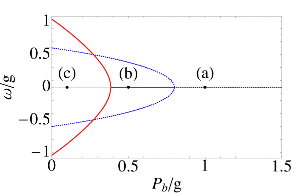
Figure 10: (Color online) Rabi slitting at resonance (dotted blue) $\pm R_{0}$, eqn (29), and the observed position of the peaks in the PL spectra (solid red) as a function of $P_{b}/g$. Parameters are those of the line of points (a), (b) and (c) of Fig. 9: $\gamma_{a}=3.8g$, $\gamma_{b}=0.1g$, $P_{a}=0.5g$, and the corresponding $P_{b}$.

The last region of SC, labelled 3, is that specified by $4g+\gamma_{b}<\gamma_{a}<4g+\gamma_{b}+P_{a}-P_{b}$, i.e., that which satisfies eqn (51) but violates eqn (50), thereby being in SC according to the more general definition that takes into account the effect of the incoherent pumping, but that, according to the conventional criterion, is in WC. For this reason, we refer to this region as of pump-aided strong coupling. This is a region of strong qualitative modification of the system, that should be in WC according to the system parameters, but that restores SC thanks to the cavity photons forced into the system.

We now consider the other side of the blue line, that displays the counterpart behaviours in the WC. Region I is that of WC in its most natural expression. Region II, in light, is the extension into WC of the characteristic of featuring two maxima in the emission spectrum. In this case, this does not correspond to a line-splitting in the sense of SC where each peak is assigned to a renormalized (dressed) state, but rather to a resonance of the Fano type that is carving a hole in the single line of the weakly-coupled system. In this region, one needs to be cautious not to read SC after the presence of two peaks at resonance. Finally, region III is the counterpart of 3, in the sense that this region is in SC according to the conventional criterion, eqn (50), for the system parameters, when in reality the too-high electronic pumping has bleached the strong-coupling.

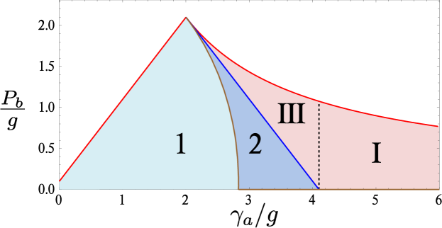
Figure 11: (Color online) The same phase space of SC/WC as in Fig. 9 as a function of $P_{b}/g$ and $\gamma_{a}/g$, only with $P_{a}/g$ now set to zero (no cavity pumping). The triangle of strong coupling is displaced, and the regions of one peak spectra (regions 2 of SC and I of WC) are enlarged, following eqn (56). As a result regions 3 and II have disappeared.

In inset, we reproduce the diagram to position the five points (a)–(e) in the various regions discussed, for which the luminescence spectra are displayed and decomposed into their Lorentzian and dispersive contributions, eqns (39). Case (c), at the lower-left angle, corresponds to SC without any pathology nor surprise: the doublet in the luminescence spectrum—although displaced in position as shown in Fig. 10—is a faithful representation of the underlying Rabi-splitting. Increasing pumping brings the system into region 2 where, albeit still in SC, it does not feature a doublet anymore. The reason why, is clear on the corresponding decomposition of the spectrum, Fig. 9(b), with a broadening of the dressed states (in purple) too large as compared to their splitting. Further increasing the pump brings it out of the SC region to reach point (a), where the two Lorentzians have collapsed. This degeneracy of the mode emission means that the coupling only affects perturbatively each mode. As a result, the dispersive correction has vanished, and the spectrum now decomposes into two new Lorentzians centred at zero, with opposite signs.

Back to point (c), now keeping the pump constant and increasing $\gamma_{a}$, we reach point (d). It is still in SC, although the cavity dissipation is very large (more than four times the coupling strength) for the small value of $\gamma_{b}$ considered. Its spectrum of emission shows, however, a clear line-splitting that is made neatly visible thanks to the cavity (residual) pumping $P_{a}$. Increasing further the dissipation eventually brings the system into WC, but in region II where, again due to $P_{a}\neq 0$, the spectrum remains a doublet. In Fig. (e), one can see, however, that there is no Rabi splitting, and that the two peaks arise as a result of a subtraction of the two Lorentzians centred at zero [see the WC spectrum decomposition in eqn (IV-41a)]. There is probably no need to display a spectrum from region I, as in this case it does not show any qualitative difference as compared to that of (a).

The set of system parameters and the estimated effective pumping rates allow to reconstruct Fig. 9 through eqn (52–56), that contains all the physics of the system. In the following, we shall look at variations of this representation to clarify or illustrate those aspects that have been amply discussed before.

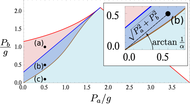
Figure 12: (Color online) Phase space of SC/WC as a function of the pumps $P_{b}/g$ and $P_{a}/g$ for fixed decay parameters $\gamma_{a}=3.8g$ and $\gamma_{b}=0.1g$. As in Fig. 9, the red lines mark the physical regions and the blue one the SC (blue shades)/WC (red shades) transition, with the same regions 1 and 2 of SC and III of WC, also with the points (a), (b) and (c), of Fig. 9. In inset, zoom of the low-pump region, showing the importance of both the angle, $\arctan{(1/\alpha)}$, and the magnitude, $\sqrt{P_{a}^{2}+P_{b}^{2}}$, of a given point.

Fig. 11 shows the same diagram as that of Fig. 9, only with $P_{a}$ now set to zero, i.e., corresponding to the case of a very clean sample with no spurious QDs other than the SC coupled one, that experiences only an electronic pumping. Observe how, as a consequence, region 3 of SC and II of WC have disappeared. The former was indeed the result of the residual cavity photons helping SC. The “pathology” in WC of featuring two peaks at resonance in WC has also disappeared, but most importantly, see how region 2 has considerably increased inside the “triangle” of strong-coupling, meaning that the parameters required so that the line-splitting can still be resolved in the luminescence spectrum now put much higher demands on the quality of the structure. This difficulty, especially in the region where $P_{b}\ll g$ follows from the “effective quantum state in the steady state”, that we have already discussed. The presence of a cavity pumping, even if it is so small that no field-intensity effects are accounted for, can favour SC by making it visible, indeed by merely providing a photon-like character to the quantum state. This is the manifestation in a SS of the same influence that was observed in the SE: the luminescence spectrum of a photon as an initial state of the coupled system, is more visible than that of an exciton, keeping all parameters otherwise the same (see Fig. 6). Another useful picture to highlight this last point, is that where the various regions are plotted in terms of the pumping rates, $P_{a}$ and $P_{b}$ [see Fig. 12, for the case $\gamma_{a}=3.8g$ of the line (a)–(c) in Fig. (9)]. The angle of a given point with the horizontal, linked to $\alpha^{-1}=P_{b}/P_{a}$, defines the exciton-like or photon-like character of the SS established in the system, and thus determines the visibility of the double-peak structure of SC. This is, at low pumpings, independent of the magnitude $\sqrt{P_{a}^{2}+P_{b}^{2}}$, as the brown line defined by eqn (56) is approximately linear in this region. This shows the importance of a careful determination of the quantum state that is established in the SS by the interplay of the pumping and decay rates, through eqn (12). The magnitude, on the other hand, affects the splitting $R_{0}$, and the linewidths $\Gamma_{+}$. In order to have a noticeable renormalization, the pumps must be comparable to the decays. On the one hand, the Rabi frequency can be affected in different ways by the pumpings, depending on the parameters. If $\Gamma_{a}=\Gamma_{b}$, there is, in general, no effect of decoherence on the splitting, showing that in this case there is a perfect symmetric coupling of the modes into the new eigenstates (although the broadening can be large and spoil the resolution of the Rabi splitting anyway). If they are different, for example in the common situation that $\gamma_{a}-\gamma_{b}>P_{a}-P_{b}$, the Rabi increases with increasing $P_{a}-P_{b}$. On the other hand, the linewidth $\Gamma_{+}=(\gamma_{a}+\gamma_{b}-P_{a}-P_{b})/4$ presents clear bosonic characteristics: it increases with the decays but narrows with pumping Scully and Zubairy (2002). The intensity of the pumps also affects the total intensity of the spectra, that is proportional to $n^{\mathrm{SS}}_{a}$ through $\gamma_{a}$ and the integration time of the apparatus. Here, however, we have focused on the normalised spectra (i.e., the lineshape).

V Summary and Conclusions

In conclusion, we have brought under a unified formalism the zero-dimensional light-matter interaction, both in the Weak (WC) and Strong (SC) Coupling, for the two cases of Spontaneous Emission (SE) of an initial state, and emission under a Steady State (SS) maintained by an incoherent, continuous pumping. While the SE case for some particular initial conditions (excited state of the atom) and configurations (resonance, direct emission) has been a pillar of SC in cQED of atoms in cavities, the extensions that we provided here to include a continuous and incoherent pumping, are suitable to describe the recent field of cQED in semiconductor heterostructures. Together, they merge into an elegant and complementary theoretical edifice.

The main results of this papers are to be found in eqns (30)–(33) that provide the analytical expression for the cavity emission spectra of a system whose specificities—such as whether it corresponds to SE or the SS established by an incoherent continuous pumping—are provided by a parameter $D$, which, in the first (SE) case, is given by eqn (34), and in the second (SS), by eqn (36). These formulas, that allow for an arbitrary detuning between the bare modes, reduce to more self-contained expressions at resonance, namely eqn (43) for SE and eqn (49) for SS. The resonance case allows an unambiguous definition of SC, depending on whether the complex Rabi frequency, eqn (28), is pure imaginary (WC) or real (SC). This corresponds, in turn, to a damping or to sustained oscillations of the time-autocorrelation of the fields. This is completely independent of the dynamics of the populations. SC is characterised by the emergence of new eigenstates, with different energies, whereas in WC, the energies remain degenerate. There is no, however, one-to-one mapping of this splitting of the energies with the lines observed in the luminescence spectrum. All cases can arise: one or two peaks can be observed at resonance both in WC and SC. In the SC case, one peak only is observed when the energy splitting is too small as compared to the broadening of the lines, whereas in the WC, two peaks are seen as a result of a resonance carving a hole in a single line, giving the illusion of a doublet (and indeed of an anticrossing when detuning is varied). For that reason, an understanding of the general picture is required to be able to position a particular experiment in the space of parameters, as was done in Fig. 9 and Figs. 11–12, rather than to rely on a qualitative effect of anticrossing at resonance. Figure 10 shows how loosely related are the observed line-splitting in the luminescence spectrum (solid red) and the actual energy splitting of the polariton modes (dressed states, in dotted blue). The various situations that may arise are illustrated and discussed in Fig. 9. The respective effects of the angle and the distance to origin in the $P_{a}$, $P_{b}$ parameter-space, is shown in Fig. 12: the angle accounts for the effective quantum state, that imparts on the visibility of the splitting in the spectrum, while the magnitude accounts for bosonic effects like line-narrowing and field-intensity renormalization of the Rabi splitting.

This work addresses the case of bosonic excitons, that corresponds to the case of vanishing excitations, even for genuine two-level excitons. As such, it also contains a lot of the physics of ground state quantum wells excitons in planar cavities, although in this case, another type of pumping—a so-called cross-terms pumping—is more adequate, as particles are injected directly into the ground state by scattering of polaritons. On the contrary, in our present scheme, the excitation is in terms of the bare modes, through phonon-assisted scattering of electron-hole pairs into the QD for the electronic pumping, $P_{b}$, or via Purcell-emission of weakly-coupled spectator dots into the cavity mode for the cavity pumping, $P_{a}$. A natural extension of this work is to consider fermionic excitons, that do not admit more than one particle. In this case, the equations of motions for the correlators are not closed, and only semi-analytical results are available. The structure of the spectra—that in the bosonic case decompose as a Lorentzian and a dispersive line for each peak—becomes that of an infinite series of lines, tightly grouped together, to give rise to multiplet structures with no more than four peaks, albeit in a wide variety of different configurations. This fermionic case corresponds to mapping the Jaynes-Cummings ladder to an exact luminescence spectrum, in much the same way that we have been doing with the Rabi doublet in this text. This case that is of crucial importance for the study of nonlinearity of genuine (two-levels) QDs in semiconductor microcavities, is the subject of part II of this text.

Appendix A Time-resolved dynamics in the SE case

From eqn (12), the mean photon population for the SE of a system whose initial conditions are given by eqn (13), is:

$$n_{a}(t)=e^{-2\gamma_{+}t}\Bigg{\{} \Big{[}\cos{(\sqrt{2}z_{1}t)}+\cosh{(\sqrt{2}z_{2}t})\Big{]}\frac{n_{a}^{0}}{2}$$ (57)

$$- \Big{[}\cos{(\sqrt{2}z_{1}t)}-\cosh{(\sqrt{2}z_{2}t)}\Big{]}\frac{(\frac{\Delta^{2}}{4}+\gamma_{-}^{2})n_{a}^{0}+g^{2}n_{b}^{0}+g\Delta\Re{n_{ab}^{0}}-2g\gamma_{-}\Im{n_{ab}^{0}}}{2|R|^{2}}$$

$$+ \left[\frac{\sin{(\sqrt{2}z_{1}t)}}{\sqrt{2}z_{1}}+\frac{\sinh{(\sqrt{2}z_{2}t})}{\sqrt{2}z_{2}}\right]\left(g\Im{n_{ab}^{0}}-\gamma_{-}n_{a}^{0}\right)$$

$$+ \left[\frac{\sin{(\sqrt{2}z_{1}t)}}{\sqrt{2}z_{1}}-\frac{\sinh{(\sqrt{2}z_{2}t})}{\sqrt{2}z_{2}}\right]\times$$ (58)

$$\qquad\frac{\gamma_{-}(\frac{\Delta^{2}}{4}+\gamma_{-}^{2}-g^{2})n_{a}^{0}+g\Delta\gamma_{-}\Re{n_{ab}^{0}}+g(\frac{\Delta^{2}}{4}-\gamma_{-}^{2}+g^{2})\Im{n_{ab}^{0}}}{|R|^{2}}\Bigg{\}}$$

The expression for $n_{b}(t)$ follows from $a\leftrightarrow b$. The crossed mean value that reflects the coherent coupling reads:

$$n_{ab}(t)=e^{-2\gamma_{+}t}\Bigg{\{}\Big{[}\cos{(\sqrt{2}z_{1}t)}+\cosh{(\sqrt{2}z_{2}t})\Big{]}\frac{n_{ab}^{0}}{2}$$ (59)

$$- \Big{[}\cos{(\sqrt{2}z_{1}t)}-\cosh{(\sqrt{2}z_{2}t)}\Big{]}\frac{g(\frac{\Delta}{2}+i\gamma_{-})n_{a}^{0}-g(\frac{\Delta}{2}-i\gamma_{-})n_{b}^{0}-(\frac{\Delta^{2}}{4}+\gamma_{-}^{2})n_{ab}^{0}+g^{2}(n_{ab}^{0})^{*}}{2|R|^{2}}$$

$$+ \left[\frac{\sin{(\sqrt{2}z_{1}t)}}{\sqrt{2}z_{1}}+\frac{\sinh{(\sqrt{2}z_{2}t})}{\sqrt{2}z_{2}}\right]\frac{i(\Delta n_{ab}^{0}-g(n_{a}^{0}-n_{b}^{0}))}{2}$$

$$+ \left[\frac{\sin{(\sqrt{2}z_{1}t)}}{\sqrt{2}z_{1}}-\frac{\sinh{(\sqrt{2}z_{2}t})}{\sqrt{2}z_{2}}\right]\times$$ (60)

$$\qquad\frac{g(\Delta\gamma_{-}-i(\frac{\Delta}{2}+g^{2}-\gamma_{-}^{2}))n_{a}^{0}+g(\Delta\gamma_{-}+i(\frac{\Delta}{2}+g^{2}-\gamma_{-}^{2}))n_{b}^{0}+i\Delta(\frac{\Delta^{2}}{4}+\gamma_{-}^{2}+g^{2})n_{ab}^{0}}{2|R|^{2}}\Bigg{\}}$$

where we have defined the complex parameters:

$$z_{1,2}= \sqrt{|R|^{2}\pm(g^{2}-\gamma_{-}^{2}+\frac{\Delta^{2}}{4})}\,.$$ (61)

In case of SC, at resonance, ($g>|\gamma_{-}|$), both $z_{1,2}$ are real, due to the fact that $|R|^{2}>|\gamma_{-}\Delta|$ for whatever the detuning, and they can be written in a more transparent way:

$$z_{1,2}=|R|\sqrt{1\pm\sqrt{1-\left(\frac{\gamma_{-}\Delta}{|R|^{2}}\right)^{2}}}\,.$$ (62)

The mean value $n_{a}(t)$ is plotted in Fig. 6(b) and 7(c) for SC and WC, respectively, for the parameters in the caption.

It might be of interest to note that eqns (57–59), but also eqn (27) in the SE case, and therefore all the results that follow from them, are reproduced by introducing decay as an imaginary part to the energies in the Heisenberg picture, i.e., upgrading $\omega_{a,b}$ to $\omega_{a,b}-i\gamma_{a,b}/2$ and solving directly in a full Hamiltonian picture the operator equations of motion: $\partial_{t}c(t)=i[H,c(t)]$ with $c=a,b$. This simple expedient resurges plainly for instance in eqn (28), that is an exact and important result derived with the full dissipative formalism, but which follows directly from eqn (6) with complex energies. This recourse to complex energies is however not valid in the Schrödinger picture and/or with the pumping terms.

Appendix B Derivation of the luminescence spectrum in the SS from the general expression

Expression (16) is general, but its final form in term of a time-integrated Fourier transforms of $G^{(1)}$, eqn (19), is not rigorous for the SS case since both the numerator and the denominator are infinite quantities. Their ratio, however, produces a finite quantity, which bears all the characteristic of the optical emission spectrum in a SS, and—may be more convincingly—recovers the well-established and rigorously derived Wiener-Khintchine formula, eqn (20). Note that this formula is, strictly speaking, an arcane mathematical result in the theory of stochastic processes. There, $S(\omega)$ is a mesure of the strength of the fluctuations of the Fourier component at frequency $\omega$ Mandel and Wolf (1995). It has no strict connection with a physical signal, as both infinite negative and positive times are required for its demonstration, which violates causality among other things. For a rigorous and extended discussion of a physical optical spectrum, see the excellent discussion by Eberly and Wódkiezicw Eberly and Wódkiewicz (1977). As the step from the general eqn (16) to the SS, eqn (20), can be made straightforwardly, we provide it below: it merely consists in cancelling the diverging quantities by obtaining the final result as a limit of the time-integrated spectrum. We believe that the starting point being so clear mathematically, and this presentation so satisfying in its simultaneous coverage of both the SE and SS cases, it is worth considering for a pedagogical purpose.

The population and the autocorrelator can be decomposed as a transient (TR) and steady-state (SS) values:

$$\langle{a^{\dagger}}a\rangle(t) =\langle{a^{\dagger}}a\rangle^{\mathrm{TR}}(t)+\lim_{t\rightarrow\infty}\langle{a^{\dagger}}a\rangle(t)\,,$$ (63a)

$$G^{(1)}(t,\tau) =\langle{a^{\dagger}}(t)a(t+\tau)\rangle^{\mathrm{TR}}+\lim_{t\rightarrow\infty}\langle{a^{\dagger}}(t)a(t+\tau)\rangle\,,$$ (63b)

where $\lim_{t\rightarrow\infty}\langle{a^{\dagger}}a\rangle(t)=n_{a}^{\mathrm{SS}}$, cf. eqn (14a). We rewrite eqn (19) as the time integration of the Fourier transform until time $T$, that is left to increase without bounds:

$$S(\omega)=\lim_{T\rightarrow\infty}\frac{1}{\pi\int_{0}^{T}\langle{a^{\dagger}}a\rangle(t)dt}\Re\int_{t=0}^{T}\int_{\tau=0}^{\infty}G^{(1)}(t,\tau)e^{i\omega\tau}\,d\tau dt\,.$$ (64)

Substituting eqns (63) in this expression, we can keep track of the terms that cancel (one can check, from the explicit results of the text, the convergence of the quantities $N\equiv\int_{0}^{\infty}\langle{a^{\dagger}}a\rangle^{\mathrm{TR}}(t)dt$ and $M_{\tau}=\int_{0}^{\infty}\langle{a^{\dagger}}(t)a(t+\tau)\rangle^{\mathrm{TR}}e^{i\omega\tau}\,dt$, for all $\tau>0$):

$$S^{\mathrm{SS}}(\omega)=\frac{1}{\pi}\lim_{T\rightarrow\infty}\frac{1}{N+Tn_{a}^{\mathrm{SS}}}\Re\int_{\tau=0}^{\infty}\bigg{[}M_{\tau}+T\lim_{t\rightarrow\infty}\langle{a^{\dagger}}(t)a(t+\tau)\rangle\bigg{]}e^{i\omega\tau}d\tau\,.$$ (65)

Since the norm of the Fourier transform of $M_{\tau}$ is also bounded (that, again, can be checked from the explicit result), the limit in $T$ yields:

$$S^{\mathrm{SS}}(\omega)=\frac{1}{\pi}\frac{1}{n_{a}^{\mathrm{SS}}}\lim_{t\rightarrow\infty}\Re\int_{0}^{\infty}\langle{a^{\dagger}}(t)a(t+\tau)\rangle e^{i\omega\tau}d\tau\,,$$ (66)

which is the formula of the text, eqn (20).

References

- Purcell (1946) E. M. Purcell, Phys. Rev. 69, 681 (1946).
- Kleppner (1981) D. Kleppner, Phys. Rev. Lett. 47, 233 (1981).
- Goy et al. (1983) P. Goy, J. M. Raimond, M. Gross, and S. Haroche, Phys. Rev. Lett. 50, 1903 (1983).
- Gérard et al. (1998) J.-M. Gérard, B. Sermage, B. Gayral, B. Legrand, E. Costard, and V. Thierry-Mieg, Phys. Rev. Lett. 81, 1110 (1998).
- Kiraz et al. (2002) A. Kiraz, S. Fälth, C. Becher, B. Gayral, W. V. Schoenfeld, P. M. Petroff, L. Zhang, E. Hu, and A. Ĭmamoḡlu, Phys. Rev. B 65, 161030(R) (2002).
- Hopfield (1958) J. J. Hopfield, Phys. Rev. 112, 1555 (1958).
- Jaynes and Cummings (1963) E. Jaynes and F. Cummings, Proc. IEEE 51, 89 (1963).
- Rudin and Reinecke (1999) S. Rudin and T. L. Reinecke, Phys. Rev. B 59, 10227 (1999).
- Dicke (1954) R. H. Dicke, Phys. Rev. 93, 99 (1954).
- Bienert et al. (2004) M. Bienert, W. Merkel, and G. Morigi, Phys. Rev. A 69, 013405 (2004).
- Carmichael (2002) H. J. Carmichael, Statistical methods in quantum optics 1 (Springer, 2002), 2nd ed.
- Carmichael et al. (1989) H. J. Carmichael, R. J. Brecha, M. G. Raizen, H. J. Kimble, and P. R. Rice, Phys. Rev. A 40, 5516 (1989).
- del Valle et al. (2008) E. del Valle, F. P. Laussy, and C. Tejedor, to be submitted (2008).
- Laussy et al. (2008) F. Laussy, E. del Valle, and C. Tejedor, arXiv:0711.1894v3 (2008).
- Rubo et al. (2003) Y. G. Rubo, F. P. Laussy, G. Malpuech, A. Kavokin, and P. Bigenwald, Phys. Rev. Lett. 91, 156403 (2003).
- Gardiner (1991) G. Gardiner, Quantum Noise (Springer-Verlag, Berlin, 1991).
- Scully and Zubairy (2002) M. O. Scully and M. S. Zubairy, Quantum optics (Cambridge University Press, 2002).
- Alicki (1988) R. Alicki, Phys. Rev. A 40, 4077 (1988).
- Mandel and Wolf (1995) L. Mandel and E. Wolf, Optical coherence and quantum optics (Cambridge University Press, 1995).
- Andreani et al. (1999) L. C. Andreani, G. Panzarini, and J.-M. Gérard, Phys. Rev. B 60, 13276 (1999).
- del Valle et al. (2007) E. del Valle, F. P. Laussy, F. Troiani, and C. Tejedor, Phys. Rev. B 76, 235317 (2007).
- Reithmaier et al. (2004) J. P. Reithmaier, G. Sek, A. Löffler, C. Hofmann, S. Kuhn, S. Reitzenstein, L. V. Keldysh, V. D. Kulakovskii, T. L. Reinecker, and A. Forchel, Nature 432, 197 (2004).
- Yoshie et al. (2004) T. Yoshie, A. Scherer, J. Heindrickson, G. Khitrova, H. M. Gibbs, G. Rupper, C. Ell, O. B. Shchekin, and D. G. Deppe, Nature 432, 200 (2004).
- Peter et al. (2005) E. Peter, P. Senellart, D. Martrou, A. Lemaître, J. Hours, J. M. Gérard, and J. Bloch, Phys. Rev. Lett. 95, 067401 (2005).
- Laussy et al. (2004) F. P. Laussy, G. Malpuech, A. Kavokin, and P. Bigenwald, Phys. Rev. Lett. 93, 016402 (2004).
- Eberly and Wódkiewicz (1977) J. Eberly and K. Wódkiewicz, J. Opt. Soc. Am. 67, 1252 (1977).