On the localized phase of a copolymer in an emulsion: subcritical percolation regime

Abstract

The present paper is a continuation of [6]. The object of interest is a two-dimensional model of a directed copolymer, consisting of a random concatenation of hydrophobic and hydrophilic monomers, immersed in an emulsion, consisting of large blocks of oil and water arranged in a percolation-type fashion. The copolymer interacts with the emulsion through an interaction Hamiltonian that favors matches and disfavors mismatches between the monomers and the solvents, in such a way that the interaction with the oil is stronger than with the water.

The model has two regimes, supercritical and subcritical, depending on whether the oil blocks percolate or not. In [6] we focussed on the supercritical regime and obtained a complete description of the phase diagram, which consists of two phases separated by a single critical curve. In the present paper we focus on the subcritical regime and show that the phase diagram consists of four phases separated by three critical curves meeting in two tricritical points.

AMS 2000 subject classifications. 60F10, 60K37, 82B27.
Key words and phrases. Random copolymer, random emulsion, localization, delocalization, phase transition, percolation, large deviations.
Acknowledgment. NP was supported by a postdoctoral fellowship from the Netherlands Organization for Scientific Research (grant 613.000.438).

1 Introduction and main results

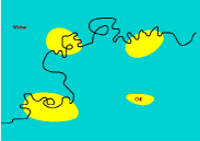
Figure 1: An undirected copolymer in an emulsion.

1.1 Background

In the present paper we consider a two-dimensional model of a random copolymer in a random emulsion (see Fig. 1) that was introduced in den Hollander and Whittington [4]. The copolymer is a concatenation of hydrophobic and hydrophilic monomers, arranged randomly with density $\frac{1}{2}$ each. The emulsion is a collection of droplets of oil and water, arranged randomly with density $p$, respectively, $1-p$, where $p\in(0,1)$. The configurations of the copolymer are directed self-avoiding paths on the square lattice. The emulsion acts as a percolation-type medium, consisting of large square blocks of oil and water, with which the copolymer interacts. Without loss of generality we will assume that the interaction with the oil is stronger than with the water.

In the literature most work is dedicated to a model where the solvents are separated by a single flat infinite interface, for which the behavior of the copolymer is the result of an energy-entropy competition. Indeed, the copolymer prefers to match monomers and solvents as much as possible, thereby lowering its energy, but in order to do so it must stay close to the interface, thereby lowering its entropy. For an overview, we refer the reader to the theses by Caravenna [1] and Pétrélis [7], and to the monograph by Giacomin [2].

With a random interface as considered here, the energy-entropy competition remains relevant on the microscopic scale of single droplets. However, it is supplemented with the copolymer having to choose a macroscopic strategy for the frequency at which it visits the oil and the water droplets. For this reason, a percolation phenomenon arises, depending on whether the oil droplets percolate or not. Consequently, we must distinguish between a supercritical regime $p\geq p_{c}$ and a subcritical regime $p<p_{c}$, with $p_{c}$ the critical probability for directed bond percolation on the square lattice.

As was proven in den Hollander and Whittington [4], in the supercritical regime the copolymer undergoes a phase transition between full delocalization into the infinite cluster of oil and partial localization near the boundary of this cluster. In den Hollander and Pétrélis [6] it was shown that the critical curve separating the two phases is strictly monotone in the interaction parameters, the phase transition is of second order, and the free energy is infinitely differentiable off the critical curve.

The present paper is dedicated to the subcritical regime, which turns out to be considerably more complicated. Since the oil droplets do not percolate, even in the delocalized phase the copolymer puts a positive fraction of its monomers in the water. Therefore, some parts of the copolymer will lie in the water and will not localize near the oil-water-interfaces at the same parameter values as the other parts that lie in the oil.

We show that there are four different phases (see Fig. 2):

• If the interaction between the two monomers and the two solvents is weak, then the copolymer is fully delocalized into the oil and into the water. This means that the copolymer crosses large clusters of oil and water alternately, without trying to follow the interfaces between these clusters. This phase is denoted by ${\mathcal{D}}_{1}$ and was investigated in detail in [4].

• If the interaction strength between the hydrophobic monomers and the two solvents is increased, then it becomes energetically favorable for the copolymer, when it wanders around in a water cluster, to make an excursion into the oil before returning to the water cluster. This phase is denote by ${\mathcal{D}}_{2}$ and was not noticed in [4].

• If, subsequently, the interaction strength between the hydrophilic monomers and the two solvents is increased, then it becomes energetically favorable for the copolymer, before moving into water clusters, to follow the oil-water-interface for awhile. This phase is denoted by ${\mathcal{L}}_{1}$.

• If, finally, the interaction between the two monomers and the two solvents is strong, then the copolymer becomes partially localized and tries to move along the oil-water interface as much as possible. This phase is denoted by ${\mathcal{L}}_{2}$.

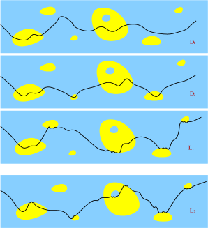
Figure 2: Typical configurations of the copolymer in each of the four phases.

In the remainder of this section we describe the model (Section 1.2), recall several key facts from [4] (Section 1.3), define and characterize the four phases (Section 1.4), and prove our main results about the shape of the critical curves and the order of the phase transitions (Section 1.5).

1.2 The model

The randomness of the copolymer is encoded by $\omega=(\omega_{i})_{i\in{\mathbb{N}}}$, an i.i.d. sequence of Bernoulli trials taking values $A$ and $B$ with probability $\tfrac{1}{2}$ each. The $i$-th monomer in the copolymer is hydrophobic when $\omega_{i}=A$ and hydrophilic when $\omega_{i}=B$. Partition ${\mathbb{R}}^{2}$ into square blocks of size $L_{n}\in{\mathbb{N}}$, i.e.,

$${\mathbb{R}}^{2}=\bigcup_{x\in{\mathbb{Z}}^{2}}\Lambda_{L_{n}}(x),\qquad\Lambda_{L_{n}}(x)=xL_{n}+(0,L_{n}]^{2}.$$ (1.1)

The randomness of the emulsion is encoded by $\Omega=(\Omega_{x})_{x\in{\mathbb{Z}}^{2}}$, an i.i.d. field of Bernoulli trials taking values $A$ or $B$ with probability $p$, respectively, $1-p$, where $p\in(0,1)$. The block $\Lambda_{L_{n}}(x)$ in the emulsion is filled with oil when $\Omega_{x}=A$ and filled with water when $\Omega_{x}=B$.

Let ${\mathcal{W}}_{n}$ be the set of $n$-step directed self-avoiding paths starting at the origin and being allowed to move upwards, downwards and to the right. The possible configurations of the copolymer are given by a subset of ${\mathcal{W}}_{n}$:

• ${\mathcal{W}}_{n,L_{n}}=$ the subset of ${\mathcal{W}}_{n}$ consisting of those paths that enter blocks at a corner, exit blocks at one of the two corners diagonally opposite the one where it entered, and in between stay confined to the two blocks that are seen upon entering (see Fig. 3).

The corner restriction, which is unphysical, is put in to make the model mathematically tractable. Despite this restriction, the model has physically relevant behavior.

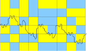
Figure 3: A directed self-avoiding path crossing blocks of oil and water diagonally. The light-shaded blocks are oil, the dark-shaded blocks are water. Each block is $L_{n}$ lattice spacings wide in both directions. The path carries hydrophobic and hydrophilic monomers on the lattice scale, which are not indicated.

Pick $\alpha,\beta\in{\mathbb{R}}$. For $\omega$, $\Omega$ and $n$ fixed, the Hamiltonian $H_{n,L_{n}}^{\omega,\Omega}(\pi)$ associated with $\pi\in{\mathcal{W}}_{n,L_{n}}$ is given by $-\alpha$ times the number of $AA$-matches plus $-\beta$ times the number of $BB$-matches. For later convenience, we add the constant $\frac{1}{2}\alpha n$, which, by the law of large numbers for $\omega$, amounts to rewriting the Hamiltonian as

$$H_{n,L_{n}}^{\omega,\Omega}(\pi)=\sum_{i=1}^{n}\Big{(}\alpha\,1\left\{\omega_{i}=A\right\}-\beta\,1\left\{\omega_{i}=B\right\}\Big{)}\,1\left\{\Omega^{L_{n}}_{(\pi_{i-1},\pi_{i})}=B\right\},$$ (1.2)

where $(\pi_{i-1},\pi_{i})$ denotes the $i$-th step in the path $\pi$ and $\Omega^{L_{n}}_{(\pi_{i-1},\pi_{i})}$ denotes the label of the block this step lies in. As shown in [4], Theorem 1.3.1, we may without loss of generality restrict the interaction parameters to the cone

$${\hbox{\footnotesize\rm CONE}}=\{(\alpha,\beta)\in{\mathbb{R}}^{2}\colon\,\alpha\geq|\beta|\}.$$ (1.3)

A path $\pi\in{\mathcal{W}}_{n,L_{n}}$ can move across four different pairs of blocks. We use the labels $k,l\in\{A,B\}$ to indicate the type of the block that is diagonally crossed, respectively, the type of the neighboring block that is not crossed. The size $L_{n}$ of the blocks in (1.1) is assumed to satisfy the conditions

$$L_{n}\to\infty\quad\mbox{ and }\quad\frac{1}{n}\,L_{n}\to 0\qquad\text{as }n\to\infty,$$ (1.4)

i.e., both the number of blocks visited by the copolymer and the time spent by the copolymer in each pair of blocks tend to infinity. Consequently, the copolymer is self-averaging w.r.t. both $\Omega$ and $\omega$.

1.3 Free energies and variational formula

In this section we recall several key facts about free energies from [4], namely, the free energy of the copolymer near a single flat infinite interface (Section 1.3.1), in a pair of neighboring blocks (Section 1.3.2), respectively, in the emulsion (Section 1.3.3).

1.3.1 Free energy near a single interface

Consider a copolymer in the vicinity of a single flat infinite interface. Suppose that the upper halfplane is oil and the lower halfplane, including the interface, is water. For $c\geq b>0$ and $L\in{\mathbb{N}}$, let ${\mathcal{W}}_{cL,bL}$ be the set of $cL$-step directed self-avoiding paths from $(0,0)$ to $(bL,0)$. The entropy per step of these paths is

$$\hat{\kappa}(c/b)=\lim_{L\to\infty}\frac{1}{cL}\log|{\mathcal{W}}_{cL,bL}|.$$ (1.5)

On this set of paths we define the Hamiltonian

$$H^{\omega,{\mathcal{I}}}_{cL}(\pi)=\sum_{i=1}^{cL}\Big{(}\alpha\,1\{\omega_{i}=A\}-\beta\,1\{\omega_{i}=B\}\Big{)}\,1\{(\pi_{i-1},\pi_{i})\leq 0\},$$ (1.6)

where $(\pi_{i-1},\pi_{i})\leq 0$ means that the $i$-th step lies in the lower halfplane (as in (1.2) we have added the constant $\frac{1}{2}\alpha cL$). The associated partition function is

$$Z^{\omega,{\mathcal{I}}}_{cL,bL}=\sum_{\pi\in{\mathcal{W}}_{cL,bL}}\exp\left[-H^{\omega,{\mathcal{I}}}_{cL}(\pi)\right].$$ (1.7)

It was proven in [4], Lemma 2.2.1, that

$$\lim_{L\to\infty}\frac{1}{cL}\log Z^{\omega,{\mathcal{I}}}_{cL,bL}=\phi^{\mathcal{I}}(\alpha,\beta;c/b)=\phi^{{\mathcal{I}}}(c/b)\qquad\omega-a.s.\mbox{ and in mean}$$ (1.8)

for some non-random function $\phi^{{\mathcal{I}}}\colon\,[1,\infty)\to{\mathbb{R}}$.

1.3.2 Free energy in a pair of neighboring blocks

Let ${\hbox{\footnotesize\rm DOM}}=\{(a,b)\colon\,a\geq 1+b,\,b\geq 0\}$. For $(a,b)\in{\hbox{\footnotesize\rm DOM}}$, let ${\mathcal{W}}_{aL,bL}$ be the set of $aL$-step directed self-avoiding paths starting at $(0,0)$, ending at $(bL,L)$, whose vertical displacement stays within $(-L,L]$ ($aL$ and $bL$ are integers). The entropy per step of these paths is

$$\kappa(a,b)=\lim_{L\to\infty}\frac{1}{aL}\log|{\mathcal{W}}_{aL,bL}|.$$ (1.9)

Explicit formulas for $\kappa$ and $\hat{\kappa}$ are given in [4], Section 2.1. These formulas are non-trivial in general, but can be used in some specific cases to perform exact computations.

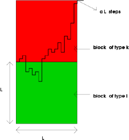
Figure 4: Two neighbouring blocks and a piece of the path. The block that is crossed is of type $k$, the block that appears as its neighbor is of type $l$.

For $k,l\in\{A,B\}$, let $\psi_{kl}$ be the quenched free energy per step of the directed self-avoiding path in a $kl$-block. Recall the Hamiltonian introduced in (1.2) and for $a\geq 2$ define (see Figure 4)

$$\psi_{kl}(\alpha,\beta;a)=\psi_{kl}(a)=\lim_{L\to\infty}\frac{1}{aL}\log\sum_{\pi\in{\mathcal{W}}_{aL,L}}\exp\big{[}-H^{\omega,\Omega}_{aL,L}(\pi)\big{]}\qquad\omega-a.s.\mbox{ and in mean}.$$ (1.10)

As shown in [4], Section 2.2, the limit exists and is non-random. For $\psi_{AA}$ and $\psi_{BB}$ explicit formulas are available, i.e.,

$$\psi_{AA}(\alpha,\beta;a)=\kappa(a,1)\quad\quad\text{and}\quad\quad\psi_{BB}(\alpha,\beta;a)=\kappa(a,1)+\frac{\beta-\alpha}{2}.$$ (1.11)

For $\psi_{AB}$ and $\psi_{BA}$ variational formulas are available involving $\phi^{{\mathcal{I}}}$ and $\kappa$. To state these let, for $a\geq 2$,

$${\hbox{\footnotesize\rm DOM}}(a)=\big{\{}(b,c)\in{\mathbb{R}}^{2}\colon\,0\leq b\leq 1,\,c\geq b,\,a-c\geq 2-b\big{\}}.$$ (1.12)

Lemma 1.1

([4], Lemma 2.2.2)
For all $a\geq 2$,

$$\psi_{BA}(a)=\sup_{(b,c)\,\in\,{\hbox{\footnotesize\rm DOM}}(a)}\frac{c\,\phi^{{\mathcal{I}}}(c/b)+(a-c)[\frac{1}{2}(\beta-\alpha)+\kappa(a-c,1-b)]}{a}.$$ (1.13)

Moreover, $\psi_{AB}$ is given by the same expression but without the term $\frac{1}{2}(\beta-\alpha)$.

Similarly, we define $\psi_{BA}^{\hat{\kappa}}$ to be the free energy per step of the paths in ${\mathcal{W}}_{aL,L}$ that make an excursion into the $A$-block before crossing diagonally the $B$-block, i.e.,

$$\psi^{\hat{\kappa}}_{BA}(a)=\sup_{(b,c)\,\in\,{\hbox{\footnotesize\rm DOM}}(a)}\frac{c\,\hat{\kappa}(c/b)+(a-c)[\frac{1}{2}(\beta-\alpha)+\kappa(a-c,1-b)]}{a}.$$ (1.14)

Since $\hat{\kappa}\leq\phi^{{\mathcal{I}}}$, we have $\psi_{BB}\leq\psi_{BA}^{\hat{\kappa}}\leq\psi_{BA}$, and these inequalities are strict in some cases. The relevant paths for (1.13–1.14) are drawn in Fig. 5.

Figure 5: Relevant paths for $\psi_{BA}$ and $\psi_{BA}^{\hat{\kappa}}$.

Remark 1.2

(1) As noted in [6], the strict concavity of $(a,b)\mapsto a\kappa(a,b)$ and $\mu\mapsto\mu\hat{\kappa}(\mu)$ together with the concavity of $\mu\mapsto\mu\phi^{{\mathcal{I}}}(\mu)$ imply that both (1.13) and (1.14) have unique maximizers, which we denote by $(\bar{b},\bar{c})$.
(2) In [6], we conjectured that $\mu\mapsto\mu\phi^{{\mathcal{I}}}(\mu)$ is strictly concave. We will need this strict concavity to prove the upper bound in Theorem 1.19 below. It implies that also $a\mapsto a\psi_{BA}(a)$ and $a\mapsto a\psi_{AB}(a)$ are strictly concave.
(3) Since $\psi_{AA}$, $\psi_{BB}$ and $\psi_{BA}^{\hat{\kappa}}$ depend on $\alpha-\beta$ and $a\in[2,\infty)$ only, we will sometimes write $\psi_{AA}(\alpha-\beta;a)$, $\psi_{BB}(\alpha-\beta;a)$ and $\psi_{BA}^{\hat{\kappa}}(\alpha-\beta;a)$.

In [4], Proposition 2.4.1, conditions were given under which $\bar{b},\bar{c}=0$ or $\neq 0$. Let

$$G(\mu,a)=\kappa(a,1)+a\partial_{1}\kappa(a,1)+\frac{a}{\mu}\,\partial_{2}\kappa(a,1)=\frac{1}{2}\left(\frac{\mu-1}{\mu}\right)\log\left(\frac{a}{a-2}\right)+\frac{1}{\mu}\log[2(a-1)],$$ (1.15)

where $\partial_{1},\partial_{2}$ denote the partial derivatives w.r.t. the first and second argument of $\kappa(a,b)$ in (1.9).

Lemma 1.3

For $a\geq 2$,

$$\psi_{AB}(a) >\psi_{AA}(a)\quad\Longleftrightarrow\quad\sup_{\mu\geq 1}\,\big{\{}\phi^{{\mathcal{I}}}(\mu)-G(\mu,a)\big{\}}>0,$$ (1.16)

$$\psi_{BA}^{\hat{\kappa}}(a) >\psi_{BB}(a)\quad\Longleftrightarrow\quad\sup_{\mu\geq 1}\,\big{\{}\hat{\kappa}(\mu)-\tfrac{1}{2}(\beta-\alpha)-G(\mu,a)\big{\}}>0.$$

1.3.3 Free energy in the emulsion

To define the quenched free energy per step of the copolymer, we put, for given $\omega,\Omega$ and $n$,

$$f_{n,L_{n}}^{\omega,\Omega} =\frac{1}{n}\log Z_{n,L_{n}}^{\omega,\Omega},$$ (1.17)

$$Z_{n,L_{n}}^{\omega,\Omega} =\sum\limits_{\pi\in{\mathcal{W}}_{n,L_{n}}}\exp\left[-H_{n,L_{n}}^{\omega,\Omega}(\pi)\right].$$

As proved in [4], Theorem 1.3.1,

$$\lim_{n\to\infty}f_{n,L_{n}}^{\omega,\Omega}=f(\alpha,\beta;p)\qquad\omega,\Omega-a.s.\mbox{ and in mean},$$ (1.18)

where, due to (1.4), the limit is self-averaging in both $\omega$ and $\Omega$. Moreover, $f(\alpha,\beta;p)$ can be expressed in terms of a variational formula involving the four free energies per pair of blocks defined in (1.10) and the frequencies at which the copolymer visits each of these pairs of blocks on the coarse-grained block scale. To state this variational formula, let $\mathcal{R}(p)$ be the set of $2\times 2$ matrices $(\rho_{kl})_{k,l\in\{A,B\}}$ describing the set of possible limiting frequencies at which $kl$-blocks are visited (see [4], Section 1.3). Let $\mathcal{A}$ be the set of $2\times 2$ matrices $(a_{kl})_{k,l\in\{A,B\}}$ such that $a_{kl}\geq 2$ for all $k,l\in\{A,B\}$, describing the times spent by the copolymer in the $kl$-blocks on time scale $L_{n}$. For $(\rho_{kl})\in{\mathcal{R}}(p)$ and $(a_{kl})\in{\mathcal{A}}$, we set

$$V\big{(}(\rho_{kl}),(a_{kl})\big{)}=\frac{\sum_{kl}\rho_{kl}a_{kl}\psi_{kl}(a_{kl})}{\sum_{kl}\rho_{kl}a_{kl}}.$$ (1.19)

Theorem 1.4

([4], Theorem 1.3.1)
For all $(\alpha,\beta)\in{\mathbb{R}}^{2}$ and $p\in(0,1)$,

$$f(\alpha,\beta;p)=\sup_{(\rho_{kl})\in{\mathcal{R}}(p)}\,\sup_{(a_{kl})\in{\mathcal{A}}}\,V\big{(}(\rho_{kl}),(a_{kl})\big{)}.$$ (1.20)

The reason why the behavior of the copolymer changes drastically at $p=p_{c}$ comes from the structure of ${\mathcal{R}}(p)$ (see Fig. 8). For $p\geq p_{c}$, the set ${\mathcal{R}}(p)$ contains matrices $(\rho_{kl})$ satisfying $\rho_{A}=\rho_{AA}+\rho_{AB}=1$, i.e., the copolymer can spend all its time inside the infinite cluster of $A$-blocks. For $p<p_{c}$, however, ${\mathcal{R}}(p)$ does not contain such matrices, and this causes that the copolymer has to cross $B$-blocks with a positive frequency. In the present paper we focus on the case $p<p_{c}$.

1.4 Characterization of the four phases

The four phases are characterized in Sections 1.4.1–1.4.4. This will involve four free energies

$$f_{{\mathcal{D}}_{1}}\leq f_{{\mathcal{D}}_{2}}\leq f_{{\mathcal{L}}_{1}}\leq f_{{\mathcal{L}}_{2}}=f,$$ (1.21)

with the inequalities becoming strict successively. We will see that the phase diagram looks like Fig. 6. Furthermore, we will see that the typical path behavior in the four phases looks like Fig. 7.

Figure 6: Sketch of the phase diagram for $p<p_{c}$.

Figure 7: Behavior of the copolymer inside the four block pairs containing oil and water for each of the four phases.

1.4.1 The ${\mathcal{D}}_{1}$-phase: $A$-delocalization and $B$-delocalization

A first region in which the free energy is analytic has been exhibited in [4]. This region corresponds to full delocalization into the $A$-blocks and $B$-blocks, i.e., when the copolymer crosses an $AB$-block or a $BA$-block it does not spend appreciable time near the $AB$-interface (see Fig. 7). Consequently, in ${\mathcal{D}}_{1}$ the free energy depends on $\alpha-\beta$ and $p$ only, since it can be expressed in terms of $\psi_{AA}$ and $\psi_{BB}$, which are functions of $\alpha-\beta$ (see Remark 1.2(3)).

Definition 1.5

For $p<p_{c}$,

$${\mathcal{D}}_{1}=\big{\{}(\alpha,\beta)\in{\hbox{\footnotesize\rm CONE}}\colon\,f(\alpha,\beta;p)=f_{{\mathcal{D}}_{1}}(\alpha-\beta;p)\big{\}}$$ (1.22)

with

$$f_{{\mathcal{D}}_{1}}(\alpha-\beta;p)=\sup_{x\geq 2,\,y\geq 2}\,\frac{\rho^{*}(p)\,x\,\psi_{AA}(x)+[1-\rho^{*}(p)]\,y\,\psi_{BB}(y)}{\rho^{*}(p)\,x+[1-\rho^{*}(p)]\,y},$$ (1.23)

where $\rho^{*}(p)$ is the maximal frequency at which the $A$-blocks can be crossed, defined by (see Fig. 8)

$$\rho^{*}(p)=\max_{(\rho_{kl})\in{\mathcal{R}}(p)}[\,\rho_{AA}+\rho_{AB}\,].$$ (1.24)

Figure 8: Sketch of $p\mapsto\rho^{*}(p)$.

The variational formula in (1.23) was investigated in [4], Section 2.5, where it was found that the supremum is uniquely attained at $(\overline{x},\overline{y})$ solving the equations

$$0 =\log 2+\rho\log(\overline{x}-2)+(1-\rho)\log(\overline{y}-2),$$ (1.25)

$$0 =(\alpha-\beta)+\log\left(\frac{\overline{x}(\overline{y}-2)}{\overline{y}(\overline{x}-2)}\right).$$

With the help of the implicit function theorem it was further proven that $f_{{\mathcal{D}}_{1}}$ is analytic on CONE.

The following criteria were derived to decide whether or not $(\alpha,\beta)\in{\mathcal{D}}_{1}$. The first is a condition in terms of block pair free energies, the second in terms of the single interface free energy.

Proposition 1.6

([4], Theorem 1.5.2)

$${\mathcal{D}}_{1} =\big{\{}(\alpha,\beta)\in{\hbox{\footnotesize\rm CONE}}\colon\,\psi_{BA}(\alpha,\beta;\overline{y})=\psi_{BB}(\alpha-\beta;\overline{y})\big{\}},$$ (1.26)

$${\mathcal{D}}_{1}^{c} =\big{\{}(\alpha,\beta)\in{\hbox{\footnotesize\rm CONE}}\colon\,\psi_{BA}(\alpha,\beta;\overline{y})>\psi_{BB}(\alpha-\beta;\overline{y})\big{\}}.$$

Corollary 1.7

([4], Proposition 2.4.1 and Section 4.2.2)

$${\mathcal{D}}_{1} =\Big{\{}(\alpha,\beta)\in{\hbox{\footnotesize\rm CONE}}\colon\,\sup_{\mu\geq 1}\,\{\phi^{{\mathcal{I}}}(\mu)-\tfrac{1}{2}(\beta-\alpha)-G(\mu,\overline{y})\}\leq 0\Big{\}},$$ (1.27)

$${\mathcal{D}}_{1}^{c} =\Big{\{}(\alpha,\beta)\in{\hbox{\footnotesize\rm CONE}}\colon\,\sup_{\mu\geq 1}\,\{\phi^{{\mathcal{I}}}(\mu)-\tfrac{1}{2}(\beta-\alpha)-G(\mu,\overline{y})\}>0\Big{\}}.$$

Corollary 1.7 expresses that leaving ${\mathcal{D}}_{1}$ is associated with a change in the optimal strategy of the copolymer inside the $BA$-blocks. Namely, $(\alpha,\beta)\in{\mathcal{D}}_{1}^{c}$ when it is favorable for the copolymer to make an excursion into the neighboring $A$-block before it diagonally crosses the $B$-block. This change comes with a non-analyticity of the free energy. A first critical curve divides the phase space into ${\mathcal{D}}_{1}$ and ${\mathcal{D}}_{1}^{c}$ (see Fig. 6).

1.4.2 The ${\mathcal{D}}_{2}$-phase: $A$-delocalization, $BA$-delocalization

Starting from $(\alpha,\beta)\in{\mathcal{D}}_{1}$ with $\beta\leq 0$, we increase $\alpha$ until it becomes energetically advantageous for the copolymer to spend some time in the $A$-solvent when crossing a $BA$-block. It turns out that the copolymer does not localize along the $BA$-interface, but rather crosses the interface to make a long excursion inside the $A$-block before returning to the $B$-block to cross it diagonally (see Fig. 7).

Definition 1.8

For $p<p_{c}$,

$${\mathcal{D}}_{2}=\big{\{}(\alpha,\beta)\in{\hbox{\footnotesize\rm CONE}}\colon\,f_{{\mathcal{D}}_{1}}(\alpha-\beta;p)<f(\alpha,\beta;p)=f_{{\mathcal{D}}_{2}}(\alpha-\beta;p)\big{\}}$$ (1.28)

with

$$f_{{\mathcal{D}}_{2}}(\alpha-\beta;p)=\sup_{x\geq 2,\,y\geq 2,\,z\geq 2}\,\sup_{\rho\in{\mathcal{R}}(p)}\frac{\rho_{A}\,x\,\psi_{AA}(x)+\rho_{BA}\,y\,\psi^{\hat{\kappa}}_{BA}(y)+\rho_{BB}\,z\,\psi_{BB}(z)}{\rho_{A}\,x\,+\rho_{BA}\,y\,+\rho_{BB}\,z},$$ (1.29)

where $\rho_{A}=\rho_{AB}+\rho_{AA}$.

Note that $f_{{\mathcal{D}}_{2}}$ depends on $\alpha-\beta$ and $p$ only, since $\psi_{AA}$, $\psi_{BB}$ and $\psi_{BA}^{\hat{\kappa}}$ are functions of $\alpha-\beta$ (see Remark 1.2(3)). Note also that, like (1.23), the variational formula in (1.29) is explicit because we have an explicit expression for $\psi_{BA}^{\hat{\kappa}}$ via (1.14) and for $\hat{\kappa}$ and $\kappa$ via the formulas that are available from [4]. This allows us to give a characterization of ${\mathcal{D}}_{2}$ in terms of the block pair free energies and the single interface free energy. For this we need a result proven in Section 2.3, which states that, by the strict concavity of $x\mapsto x\psi_{AA}(x)$, $y\mapsto y\psi^{\hat{\kappa}}_{BA}(y)$ and $z\mapsto z\psi_{BB}(z)$, the maximizers $(\overline{x},\overline{y},\overline{z})$ of (1.29) are unique and do not depend on the choice of $(\rho_{kl})$ that achieves the maximum in (1.20).

Proposition 1.9

$${\mathcal{D}}_{2} ={\mathcal{D}}_{1}^{c}\cap\big{\{}(\alpha,\beta)\in{\hbox{\footnotesize\rm CONE}}\colon\;\psi_{AB}(\overline{x})=\psi_{AA}(\overline{x})\text{ and }\psi_{BA}(\overline{y})=\psi_{BA}^{\hat{\kappa}}(\overline{y})\big{\}},$$ (1.30)

$${\mathcal{D}}_{2}^{c} ={\mathcal{D}}_{1}\cup\big{\{}(\alpha,\beta)\in{\hbox{\footnotesize\rm CONE}}\colon\;\psi_{AB}(\overline{x})>\psi_{AA}(\overline{x})\text{ or }\psi_{BA}(\overline{y})>\psi_{BA}^{\hat{\kappa}}(\overline{y})\big{\}}.$$

Corollary 1.10

$${\mathcal{D}}_{2} ={\mathcal{D}}_{1}^{c}\cap\Big{\{}(\alpha,\beta)\in{\hbox{\footnotesize\rm CONE}}\colon\,\sup_{\mu\geq 1}\,\big{\{}\phi^{{\mathcal{I}}}(\mu)-G(\mu,\overline{x})\big{\}}\leq 0\text{ and }\phi^{{\mathcal{I}}}(\bar{c}/\bar{b})=\hat{\kappa}(\bar{c}/\bar{b})\Big{\}},$$ (1.31)

$${\mathcal{D}}_{2}^{c} ={\mathcal{D}}_{1}\cup\Big{\{}(\alpha,\beta)\in{\hbox{\footnotesize\rm CONE}}\colon\,\sup_{\mu\geq 1}\,\big{\{}\phi^{{\mathcal{I}}}(\mu)-G(\mu,\overline{x})\big{\}}>0\text{ or }\phi^{{\mathcal{I}}}(\bar{c}/\bar{b})>\hat{\kappa}(\bar{c}/\bar{b})\Big{\}},$$

where $(\bar{b},\bar{c})$ are the unique maximizers of the variational formula for $\psi^{\hat{\kappa}}_{BA}(\overline{y})$ in (1.14).

1.4.3 The ${\mathcal{L}}_{1}$-phase: $A$-delocalization, $BA$-localization

Starting from $(\alpha,\beta)\in{\mathcal{D}}_{2}$, we increase $\beta$ and enter into a third phase denoted by ${\mathcal{L}}_{1}$. This phase is characterized by a partial localization along the interface in the $BA$-blocks. The difference with the phase ${\mathcal{D}}_{2}$ is that, in ${\mathcal{L}}_{1}$, the copolymer crosses the $BA$-blocks by first sticking to the interface for awhile before crossing diagonally the $B$-block, whereas in ${\mathcal{D}}_{2}$ the copolymer wanders for awhile inside the $A$-block before crossing diagonally the $B$-block (see Fig. 7). This difference appears in the variational formula, because the free energy in the $BA$-block is given by $\psi_{BA}$ in ${\mathcal{L}}_{1}$ instead of $\psi^{\hat{\kappa}}_{BA}$ in ${\mathcal{D}}_{2}$:

Definition 1.11

For $p<p_{c}$,

$${\mathcal{L}}_{1}=\big{\{}(\alpha,\beta)\in{\hbox{\footnotesize\rm CONE}}\colon\,f_{{\mathcal{D}}_{2}}(\alpha-\beta;p)<f(\alpha,\beta;p)=f_{{\mathcal{L}}_{1}}(\alpha,\beta;p)\big{\}}$$ (1.32)

with

$$f_{{\mathcal{L}}_{1}}(\alpha,\beta;p)=\sup_{x\geq 2,\,y\geq 2,\,z\geq 2}\,\sup_{(\rho_{kl})\in{\mathcal{R}}(p)}\frac{\rho_{A}\,x\,\psi_{AA}(x)+\rho_{BA}\,y\,\psi_{BA}(y)+\rho_{BB}\,z\,\psi_{BB}(z)}{\rho_{A}\,z\,+\rho_{BA}\,y\,+\rho_{BB}\,z}.$$ (1.33)

Since the strict concavity of $x\mapsto x\psi_{BA}(x)$ has not been proven (recall Remark 1.2(2)), the maximizers $(\overline{x},\overline{y},\overline{z})$ of (1.33) are not known to be unique. However, the strict concavity of $x\mapsto x\psi_{AA}(x)$ and $z\mapsto z\psi_{BB}(z)$ ensure that at least $\overline{x}$ and $\overline{z}$ are unique.

Proposition 1.12

$${\mathcal{L}}_{1} ={\mathcal{D}}_{1}^{c}\cap{\mathcal{D}}_{2}^{c}\cap\big{\{}(\alpha,\beta)\in{\hbox{\footnotesize\rm CONE}}\colon\,\psi_{AB}(\overline{x})=\psi_{AA}(\overline{x})\big{\}},$$ (1.34)

$${\mathcal{L}}_{1}^{c} ={\mathcal{D}}_{1}\cup{\mathcal{D}}_{2}\cup\big{\{}(\alpha,\beta)\in{\hbox{\footnotesize\rm CONE}}\colon\,\psi_{AB}(\overline{x})>\psi_{AA}(\overline{x})\big{\}}.$$

Corollary 1.13

$${\mathcal{L}}_{1} ={\mathcal{D}}_{1}^{c}\cap{\mathcal{D}}_{2}^{c}\cap\Big{\{}(\alpha,\beta)\in{\hbox{\footnotesize\rm CONE}}\colon\,\sup_{\mu\geq 1}\,\{\phi^{{\mathcal{I}}}(\mu)-G(\mu,\overline{x})\}\leq 0\Big{\}},$$ (1.35)

$${\mathcal{L}}_{1}^{c} ={\mathcal{D}}_{1}\cup{\mathcal{D}}_{2}\cup\Big{\{}(\alpha,\beta)\in{\hbox{\footnotesize\rm CONE}}\colon\,\sup_{\mu\geq 1}\,\{\phi^{{\mathcal{I}}}(\mu)-G(\mu,\overline{x})\}>0\Big{\}}.$$

As asserted in Theorem 1.16 below, if we let $(\alpha,\beta)$ run in ${\mathcal{D}}_{2}$ along a linear segment parallel to the first diagonal, then the free energy $f(\alpha,\beta;p)$ remains constant until $(\alpha,\beta)$ enters ${\mathcal{L}}_{1}$. In other words, if we pick $(\alpha_{0},\beta_{0})\in{\mathcal{D}}_{2}$ and consider for $u\geq 0$ the point $s_{u}=(\alpha_{0}+u,\beta_{0}+u)$, then the free energy $f(s_{u};p)$ remains equal to $f(\alpha_{0},\beta_{0};p)$ until $s_{u}$ exits ${\mathcal{D}}_{2}$ and enters ${\mathcal{L}}_{1}$. This passage from ${\mathcal{D}}_{2}$ to ${\mathcal{L}}_{1}$ comes with a non-analyticity of the free energy. This phase transition is represented by a second critical curve in the phase diagram (see Fig. 6).

1.4.4 The ${\mathcal{L}}_{2}$-phase: $AB$-localization, $BA$-localization

The remaining phase is:

Definition 1.14

For $p<p_{c}$,

$${\mathcal{L}}_{2}=\big{\{}(\alpha,\beta)\in{\hbox{\footnotesize\rm CONE}}\colon\,f_{{\mathcal{L}}_{1}}(\alpha,\beta;p)<f(\alpha,\beta;p)\big{\}}.$$ (1.36)

Starting from $(\alpha,\beta)\in{\mathcal{L}}_{1}$, we increase $\beta$ until it becomes energetically advantageous for the copolymer to localize at the interface in the $AB$-blocks as well. This new phase has both $AB$- and $BA$-localization (see Fig. 7). Unfortunately, we are not able to show non-analyticity at the crossover from ${\mathcal{L}}_{1}$ to ${\mathcal{L}}_{2}$ because, unlike in ${\mathcal{D}}_{2}$, in ${\mathcal{L}}_{1}$ the free energy is not constant in one particular direction (and the argument we gave for the non-analyticity at the crossover from ${\mathcal{D}}_{2}$ to ${\mathcal{L}}_{1}$ is not valid here). Consequently, the phase transition between ${\mathcal{L}}_{1}$ and ${\mathcal{L}}_{2}$ is still a conjecture at this stage, but we strongly believe that a third critical curve indeed exists.

1.5 Main results for the phase diagram

In Section 1.4 we defined the four phases and obtained a characterization of them in terms of the block pair free energies and the single interface free energy at certain values of the maximizers in the associated variational formulas. The latter serve as the starting point for the analysis of the properties of the critical curves (Section 1.5.1) and the phases (Sections 1.5.2–1.5.3).

Figure 9: Further details of the phase diagram for $p<p_{c}$ sketched in Fig. 6. There are four phases, separated by three critical curves, meeting at two tricritical points.

1.5.1 Critical curves

The first two theorems are dedicated to the critical curves between ${\mathcal{D}}_{1}$ and ${\mathcal{D}}_{2}$, respectively, between ${\mathcal{D}}_{2}$ and ${\mathcal{L}}_{1}$ (see Fig. 9).

Theorem 1.15

Let $p<p_{c}$.
(i) There exists an $\alpha^{*}(p)\in(0,\infty)$ such that $(\alpha^{*}(p),0)\in{\mathcal{D}}_{1}$ and ${\mathcal{D}}_{1}\subset\{(\beta+r,\beta)\colon\;r\leq\alpha^{*}(p),\beta\geq-\tfrac{r}{2}\}$.
(ii) For all $r\in[0,\alpha^{*}(p)]$ there exists a $\beta_{c}^{1}(r)\geq 0$ such that ${\mathcal{D}}_{1}\cap\{(\beta+r,\beta)\colon\,\beta\in{\mathbb{R}}\}$ is the linear segment

$${\mathcal{J}}_{r}^{1}=\big{\{}(\beta+r,\beta)\colon\,\beta\in[-\tfrac{r}{2},\beta_{c}^{1}(r)]\big{\}}.$$ (1.37)

The free energy $f(\alpha,\beta;p)$ is constant on this segment.
(iii) $r\mapsto\beta_{c}^{1}(r)$ is continuous on $[0,\alpha^{*}(p)]$.
(iv) Along the curve $r\in(0,\alpha^{*}(p)]\mapsto(\beta_{c}^{1}(r)+r,\beta_{c}^{1}(r))$ the two phases ${\mathcal{D}}_{1}$ and ${\mathcal{L}}_{1}$ touch each other, i.e., for all $r\in(0,\alpha^{*}(p)]$ there exists a $v_{r}>0$ such that

$$\{(\beta+r,\beta)\colon\,\beta\in(\beta_{c}^{1}(r),\beta_{c}^{1}(r)+v_{r}]\}\subset{\mathcal{L}}_{1}.$$ (1.38)

(v) $\beta^{1}_{c}(r)\geq\log(1+(1-e^{-r})^{1/2})$ for all $r\in[0,\alpha^{*}(p)]$.

Theorem 1.16

Let $p<p_{c}$.
(i) For all $r\in(\alpha^{*}(p),\infty)$ there exists a $\beta_{c}^{2}(r)>0$ such that ${\mathcal{D}}_{2}\cap\{(\beta+r,\beta)\colon\,\beta\in{\mathbb{R}}\}$ is the linear segment

$${\mathcal{J}}^{2}_{r}=\big{\{}(\beta+r,\beta)\colon\,\beta\in[-\tfrac{r}{2},\beta_{c}^{2}(r)]\big{\}}.$$ (1.39)

The free energy $f(\alpha,\beta;p)$ is constant on this segment.
(ii) $r\mapsto\beta_{c}^{2}(r)$ is lower semi-continuous on $(\alpha^{*}(p),\infty)$.
(iii) At $\alpha^{*}(p)$ the following inequality holds:

$$\limsup_{r\downarrow\alpha^{*}(p)}\beta_{c}^{2}(r)\leq\beta_{c}^{1}(\alpha^{*}(p)).$$ (1.40)

(iv) There exists an $r_{2}>\alpha^{*}(p)$ such that along the interval $(\alpha^{*}(p),r_{2}]$ the two phases ${\mathcal{D}}_{2}$ and ${\mathcal{L}}_{1}$ touch each other, i.e., for all $r\in(\alpha^{*}(p),r_{2}]$ there exists a $v_{r}>0$ such that

$$\{(\beta+r,\beta)\colon\,\beta\in[\beta_{c}^{2}(r),\beta_{c}^{2}(r)+v_{r}]\}\subset{\mathcal{L}}_{1}.$$ (1.41)

(v) $\beta_{c}^{2}(r)\geq\log(1+(1-e^{-r})^{1/2})$ for all $r\in(\alpha^{*}(p),\infty)$.

In [4] it was suggested that the tricritical point where ${\mathcal{D}}_{1}$, ${\mathcal{D}}_{2}$ and ${\mathcal{L}}_{1}$ meet lies on the horizontal axis. Thanks to Theorem 1.16(iii) and (v) we now know that it lies strictly above.

1.5.2 Infinite differentiability of the free energy

It was shown in [4], Lemma 2.5.1 and Proposition 4.2.2, that $f$ is analytic on the interior of ${\mathcal{D}}_{1}$. We complement this result with the following.

Theorem 1.17

Let $p<p_{c}$. Then, under Assumption 4.3 in Section 4.3.1, $(\alpha,\beta)\mapsto f(\alpha,\beta;p)$ is infinitely differentiable on the interior of ${\mathcal{D}}_{2}$.

Consequently, there are no phase transitions of finite order in the interior of ${\mathcal{D}}_{1}$ and ${\mathcal{D}}_{2}$.

Assumption 4.3 in Section 4.3.1 concerns the first supremum in (1.20) when $(\alpha,\beta)\in{\mathcal{D}}_{2}$. Namely, it requires that this supremum is uniquely taken at $(\rho_{kl})=(\rho^{*}_{kl}(p))$ with $\rho^{*}_{AA}(p)+\rho^{*}_{AB}(p)=\rho^{*}(p)$ given by (1.24) and with $\rho^{*}_{BA}(p)$ maximal subject to the latter equality. In view of Fig. 7, this is a resonable assumption indeed, because in ${\mathcal{D}}_{2}$ the copolymer will first try to maximize the fraction of time it spends crossing $A$-blocks, and then try to maximize the fraction of time it spends crossing $B$-blocks that have an $A$-block as neighbor.

We do not have a similar result for the interior of ${\mathcal{L}}_{1}$ and ${\mathcal{L}}_{2}$, simply because we have insufficient control of the free energy in these regions. Indeed, whereas the variational formulas (1.23) and (1.29) only involve the block free energies $\psi_{AA}$, $\psi_{BB}$ and $\psi_{BA}^{\widehat{\kappa}}$, for which (1.11) and (1.14) provide closed form expressions, the variational formula in (1.33) also involves the block free energy $\psi_{BA}$, for which no closed form expression is known because (1.13) contains the single flat infinite interface free energy $\phi^{\mathcal{I}}$.

1.5.3 Order of the phase transitions

Theorem 1.15(ii) states that, in ${\mathcal{D}}_{1}$, for all $r\in[0,\alpha^{*}(p)]$ the free energy $f$ is constant on the linear segment ${\mathcal{J}}^{1}_{r}$, while Theorem 1.16(i) states that, in ${\mathcal{D}}_{2}$, for all $r\in(\alpha^{*}(p),\infty)$ the free energy $f$ is constant on the linear segment ${\mathcal{J}}_{r}^{2}$. We denote these constants by $f_{{\mathcal{D}}_{1}}(r)$, respectively, $f_{{\mathcal{D}}_{2}}(r)$.

According to Theorems 1.15(ii) and 1.16(ii), the phase transition between ${\mathcal{D}}_{1}$ and ${\mathcal{D}}_{2}$ occurs along the linear segment ${\mathcal{J}}^{1}_{\alpha^{*}(p)}$ with $\beta_{c}^{1}(\alpha^{*}(p))=\alpha^{**}(p)-\alpha^{*}(p)$. This transition is of order smaller than or equal to $2$.

Theorem 1.18

There exists a $c>0$ such that, for $\delta>0$ small enough,

$$c\,\delta^{2}\leq f_{{\mathcal{D}}_{2}}(\alpha^{*}(p)+\delta)-f_{{\mathcal{D}}_{1}}(\alpha^{*}(p))-f^{\prime}_{{\mathcal{D}}_{1}}(\alpha^{*}(p))\,\delta-\frac{1}{2}\,f^{\prime\prime}_{{\mathcal{D}}_{1}}(\alpha^{*}(p))\,\delta^{2}.$$ (1.42)

According to Theorem 1.15(iv), the phase transition between ${\mathcal{D}}_{1}$ and ${\mathcal{L}}_{1}$ occurs along the curve $\{(r+\beta_{c}^{1}(r),\beta_{c}^{1}(r))\colon\,r\in[0,\alpha^{*}(p)]\}$. This transition is of order smaller than or equal to $2$ and strictly larger than 1.

Theorem 1.19

For all $r\in[0,\alpha^{*}(p))$ there exist $c>0$ and $\zeta\colon\,[0,1]\mapsto[0,\infty)$ satisfying $\lim_{x\downarrow 0}\zeta(x)=0$ such that, for $\delta>0$ small enough,

$$c\,\delta^{2}\leq f_{{\mathcal{L}}_{1}}(r+\beta_{c}^{1}(r)+\delta,\beta_{c}^{1}(r)+\delta)-f_{{\mathcal{D}}_{1}}(r)\leq\zeta(\delta)\delta.$$ (1.43)

According to Theorem 1.16(iv), the phase transition between ${\mathcal{D}}_{2}$ and ${\mathcal{L}}_{1}$ occurs at least along the curve

$$\big{\{}(r+\beta_{c}^{2}(r),\beta_{c}^{2}(r))\colon\,r\in[\alpha^{*}(p),\alpha^{*}(p)+r_{2}]\big{\}}.$$ (1.44)

We are not able to determine the exact order of this phase transition, but we can prove that it is smaller than or equal to the order of the phase transition in the single interface model. The latter model was investigated (for a different but analogous Hamiltonian) in Giacomin and Toninelli [3], where it was proved that the phase transition is at least of second order. Numerical simulations suggest that the order is in fact higher than second order. In what follows we denote by $\gamma$ the order of the single interface transition. This means that there exist $c_{2}>c_{1}>0$ and a slowly varying function $L$ such that, for $\delta>0$ small enough,

$$c_{1}\delta^{\gamma}L(\delta)\leq\phi^{{\mathcal{I}}}(\tfrac{c_{r}}{b_{r}};r+\beta_{c}^{2}(r)+\delta,\beta_{c}^{2}(r)+\delta)-\hat{\kappa}(\tfrac{c_{r}}{b_{r}})\leq c_{2}\delta^{\gamma}L(\delta),$$ (1.45)

where $(c_{r},b_{r})$ are the unique maximizers of (1.14) at $(r+\beta_{c}^{2}(r),\beta_{c}^{2}(r);y_{r})$ and $y_{r}$ is the second component of the unique maximizers of (1.29) at $(r+\beta_{c}^{2}(r),\beta_{c}^{2}(r))$.

Theorem 1.20

For all $r\in[\alpha^{*}(p),\alpha^{*}(p)+r_{2})$ there exist $c>0$ such that, for $\delta>0$ small enough,

$$c\,\delta^{\gamma}L(\delta)\leq f_{{\mathcal{L}}_{1}}(r+\beta_{c}^{2}(r)+\delta,\beta_{c}^{2}(r)+\delta)-f_{{\mathcal{D}}_{2}}(r).$$ (1.46)

We believe that the order of the phase transition along the critical curve separating ${\mathcal{D}}_{1}$ and ${\mathcal{D}}_{2}$, ${\mathcal{D}}_{1}$ and ${\mathcal{L}}_{1}$, and ${\mathcal{D}}_{2}$ and ${\mathcal{L}}_{1}$ are, respectively, 2, 2 and $\gamma$. However, except for Theorem 1.19, in which we give a partial upper bound, we have not been able to prove upper bounds in Theorems 1.18 and 1.20 due to a technical difficulty associated with the uniqueness of the maximizer $(a_{kl})$ in (1.20).

1.6 Open problems

The following problems are interesting to pursue (see Fig. 9):

• Prove that $r\mapsto\beta_{c}^{2}(r)$ is continuous on $(\alpha^{*}(p),\infty)$. Prove that $r\mapsto\beta_{c}^{1}(r)$ is strictly decreasing and $r\mapsto\beta_{c}^{2}(r)$ is strictly increasing.

• Show that the critical curve between ${\mathcal{D}}_{2}$ and ${\mathcal{L}}_{1}$ meets the critical curve between ${\mathcal{D}}_{1}$ and ${\mathcal{D}}_{2}$ at the end of the linear segment, i.e., show that (1.40) can be strengthened to an equality.

• Establish the existence of the critical curve between ${\mathcal{L}}_{1}$ and ${\mathcal{L}}_{2}$. Prove that the free energy is infinitely differentiable on the interior of ${\mathcal{L}}_{1}$ and ${\mathcal{L}}_{2}$.

• Show that the critical curve between ${\mathcal{D}}_{2}$ and ${\mathcal{L}}_{1}$ never crosses the critical curve between ${\mathcal{L}}_{1}$ and ${\mathcal{L}}_{2}$.

• Show that the phase transitions between ${\mathcal{D}}_{1}$ and ${\mathcal{L}}_{1}$ and between ${\mathcal{D}}_{1}$ and ${\mathcal{D}}_{2}$ are of order $2$.

1.7 Outline

In Section 2 we derive some preparatory results concerning existence and uniqueness of maximizers and inequalities between free energies. These will be used in Section 3–4 to prove the claims made in Section 1.4–1.5, respectively.

The present paper concludes the analysis of the phase diagram started in [4] and continued in [6]. The results were announced in [5] without proof.

2 Preparations

2.1 smoothness of $\hat{\kappa}$ and $\kappa$

In this section, we recall some results from [4] concerning the entropies $\kappa$ and $\hat{\kappa}$ defined in (1.9) and (1.5).

Lemma 2.1

([4], Lemma 2.1.2 and 2.1.1)
(i) $(a,b)\mapsto a\kappa(a,b)$ is continuous and strictly concave on DOM and analytic on the interior of DOM.
(ii) $\mu\mapsto\mu\hat{\kappa}(\mu)$ is continuous and strictly concave on $[1,\infty)$ and analytic on $(1,\infty)$.

This allows to state the following properties of $\psi_{kl}$.

Corollary 2.2

(i) For $kl\in\{AA,BB\}$, $(\alpha,\beta,a)\mapsto\psi_{kl}(\alpha,\beta;a)$ is infinitely differentiable on $\mathbb{R}^{2}\times(2,\infty)$.
(ii) For $kl\in\{AA,BB\}$ and $(\alpha,\beta)\in{\hbox{\footnotesize\rm CONE}}$, $a\mapsto\psi_{kl}(\alpha,\beta;a)$ is strictly concave on $[2,\infty)$.
(iii) For $(\alpha,\beta)\in{\hbox{\footnotesize\rm CONE}}$, $a\mapsto\psi_{BA}^{\hat{\kappa}}(\alpha,\beta;a)$ is strictly concave $[2,\infty)$.

Proof.  Lemma 2.1 and formulas 1.11 imply immediately (i) and (ii). Lemma 2.1 implies also that for all $a\geq 2$, $(c,b)\mapsto c\kappa(c/b)$ and $(c,b)\mapsto(a-c)\kappa(a-c,1-b)$ are strictly concave. The latter, together with formula (1.14) are sufficient to obtain (iii). $\square$

2.2 Smoothness of $\phi^{{\mathcal{I}}}$ and $\psi_{kl}$

In this section, we recall from [6] some key properties concerning the single interface free energy and the block pair free energies.

Lemma 2.3

(i) $(\alpha,\beta,\mu)\mapsto\phi^{{\mathcal{I}}}(\alpha,\beta;\mu)$ is continuous on ${\hbox{\footnotesize\rm CONE}}\times[1,\infty)$.
(ii) For all $k,l\in\{A,B\}$, $(\alpha,\beta;a)\mapsto\psi_{kl}(\alpha,\beta;a)$ is continuous on ${\hbox{\footnotesize\rm CONE}}\times[2,\infty)$.

Proof.  To prove (i) it suffices to check that $\mu\mapsto\phi^{{\mathcal{I}}}(\alpha,\beta;\mu)$ is continuous on $[1,\infty)$ and that there exists a $K>0$ such that $(\alpha,\beta)\mapsto\phi^{{\mathcal{I}}}(\alpha,\beta;\mu)$ is $K$-Lipshitz for all $\mu\in[1,\infty)$. These two properties are obtained by using, respectively, the concavity of $\mu\mapsto\mu\phi^{{\mathcal{I}}}(\alpha,\beta;\mu)$ and the expression of the Hamiltonian in (1.6). The proof of (ii) is the same. $\square$

Other important results, proven in [6], are stated below. They concern the asymptotic behavior of $\psi_{kl}$, $\phi^{{\mathcal{I}}}$ and some of their partial derivatives as $\mu$ and $a$ tend to $\infty$.

Lemma 2.4

([6], Lemma 2.4.1) For any $\beta_{0}>0$, uniformly in $\alpha\geq\beta$ and $\beta\leq\beta_{0}$,
(i) $\lim_{\mu\to\infty}\phi^{\mathcal{I}}(\alpha,\beta;\mu)=0$,
(ii) for $kl\in\{AB,BA\}$, $\lim_{a\to\infty}\psi_{kl}(\alpha,\beta;a)=0$.

Lemma 2.5

([6], Lemma 5.4.3) Fix $(\alpha,\beta)\in{\hbox{\footnotesize\rm CONE}}$.
(i) For all $k,l\in\{A,B\}$ with $kl\neq BB$, $\lim_{a\to\infty}a\psi_{kl}(a)=\infty$.
(ii) Let $\mathcal{K}$ be a bounded subset of CONE. For all $k,l\in\{A,B\}$, $\lim_{a\to\infty}\partial[a\psi_{kl}(\alpha,\beta;a)]/\partial a\leq 0$ uniformly in $(\alpha,\beta)\in\mathcal{K}$.

Proof.  Only the uniformity in $(\alpha,\beta)\in\mathcal{K}$ in (ii) was not proven in [6]. This is obtained as follows. Let $m$ be the minimum of $2\psi_{kl}(\alpha,\beta;2)$ on $\mathcal{K}$. By Lemma 2.4(ii), for all ${\varepsilon}>0$ there exists an $a_{0}\geq 2$ such that $\psi_{kl}(\alpha,\beta;a)\leq{\varepsilon}$ for all $(\alpha,\beta)\in\mathcal{K}$ and $a\geq a_{0}$. Moreover, by concavity, the derivative of $a\mapsto a\psi_{kl}(\alpha,\beta;a)$ is decreasing and, consequently, $a{\varepsilon}-m\geq(a-2)\partial_{a}\psi_{kl}(\alpha,\beta;a)$ for $a\geq a_{0}$. This implies that

$$\partial_{a}\psi_{kl}(\alpha,\beta;a)\leq\frac{a{\varepsilon}-m}{a-2}=\frac{{\varepsilon}-m/a}{1-2/a},\qquad a\geq a_{0}.$$ (2.1)

$\square$

2.3 Maximizers for the free energy: existence and uniqueness

Up to now we have stated the existence and uniqueness of the maximizers of the variational formula (1.20) only in some particular cases. In ${\mathcal{D}}_{1}$ we recalled the result of [4], stating the uniqueness of the maximizers $(\overline{x},\overline{y})$ in the variational formula (1.23), while in ${\mathcal{D}}_{2}$ we announced the uniqueness of the maximizers $(\overline{x},\overline{y},\overline{z})$ in the variational formula (1.29).

For $(\alpha,\beta)\in{\hbox{\footnotesize\rm CONE}}$, $p\in(0,1)$ and $(\rho_{kl})\in{\mathcal{R}}(p)$, let (recall (1.19))

$$f_{\alpha,\beta,(\rho_{kl})} =\sup_{(a_{kl})\in{\mathcal{A}}}V\big{(}(\rho_{kl}),(a_{kl})\big{)},$$ (2.2)

$${\mathcal{O}}_{(\rho_{kl})} =\big{\{}kl\in\{A,B\}^{2}\colon\,\rho_{kl}>0\big{\}},$$

$${\mathcal{J}}_{\alpha,\beta,(\rho_{kl})} =\{(a_{kl})_{kl\in{\mathcal{O}}_{\rho}}\in{\mathcal{A}}\colon\,f_{\alpha,\beta,(\rho_{kl})}=V\big{(}(\rho_{kl}),(a_{kl})\big{)}\},$$

$${\mathcal{R}}_{\alpha,\beta,p}^{f} =\{(\rho_{kl})\in{\mathcal{R}}(p)\colon\,f(\alpha,\beta;p)=f_{\alpha,\beta,(\rho_{kl})}\},$$

$${\mathcal{P}}_{\alpha,\beta,p} =\bigcup_{(\rho_{kl})\in{\mathcal{R}}_{\alpha,\beta,p}^{f}}{\mathcal{O}}_{(\rho_{kl})}.$$

Lemma 2.6

For every $(\alpha,\beta)\in{\hbox{\footnotesize\rm CONE}}$, $p\in(0,1)$ and $(\rho_{kl})\in{\mathcal{R}}(p)$, the set ${\mathcal{J}}_{\alpha,\beta,(\rho_{kl})}$ is non-empty. Moreover, for all $kl\in{\mathcal{O}}_{(\rho_{kl})}$ such that $x\mapsto x\psi_{kl}(x)$ is strictly concave, there exists a unique $a^{(\rho_{kl})}_{kl}\geq 2$ such that $a_{kl}=a^{(\rho_{kl})}_{kl}$ for all $(a_{kl})\in{\mathcal{J}}_{\alpha,\beta,(\rho_{kl})}$.

Proof.  The proof that ${\mathcal{J}}_{\alpha,\beta,(\rho_{kl})}\neq\emptyset$ is given in [6], Proposition 5.5.1. If $(a_{kl})\in{\mathcal{J}}_{\alpha,\beta,(\rho_{kl})}$, then differentiation gives

$$\frac{\partial[x\psi_{kl}(x)]}{\partial x}(a_{kl})=f_{\alpha,\beta,(\rho_{kl})},$$ (2.3)

which implies the uniqueness of $a_{kl}$ as soon as $x\mapsto x\psi_{kl}(x)$ is strictly concave. $\square$

Remark 2.7

Note that (2.3) ought really to be written as

$$\partial^{-}[x\psi_{kl}(x)](a_{kl})\leq f_{\alpha,\beta,(\rho_{kl})}\leq\partial^{+}[x\psi_{kl}(x)](a_{kl}),$$ (2.4)

where $\partial^{-}$ and $\partial^{+}$ denote the left- and right-derivative. Indeed, for $kl\in\{AB,BA\}$ we do not know whether $x\mapsto x\psi_{kl}(x)$ is differentiable or not. However, we know that these functions are concave, which is sufficient to ensure the existence of the left- and right-derivative. We will continue this abuse of notation in what follows.

Proposition 2.8

For every $(\alpha,\beta)\in{\hbox{\footnotesize\rm CONE}}$ and $p\in(0,1)$, the set ${\mathcal{R}}^{f}_{\alpha,\beta,p}$ is non-empty. Moreover, for all $kl\in{\mathcal{P}}_{\alpha,\beta,p}$ such that $x\mapsto x\psi_{kl}(x;\alpha,\beta)$ is strictly concave, there exists a unique $a_{kl}(\alpha,\beta)\geq 2$ such that $a^{(\rho)}_{kl}=a_{kl}(\alpha,\beta)$ for all $(\rho_{kl})\in{\mathcal{R}}_{\alpha,\beta,p}^{f}$.

Proof.  We begin with the proof of ${\mathcal{R}}^{f}_{\alpha,\beta,p}\neq\emptyset$. Let $(\rho^{B})=(\rho^{B}_{kl})$ denote the $2\times 2$ matrix with $\rho^{B}_{BB}=1$ and $\rho^{B}_{BA}=\rho^{B}_{AB}=\rho^{B}_{AA}=0$.

Case 1: $\sup_{x\geq 2}\psi_{BB}(x)>0$.
Since ${\mathcal{R}}(p)$ is a compact set, the continuity of $(\rho_{kl})\mapsto f_{\alpha,\beta,(\rho_{kl})}$ implies that ${\mathcal{R}}^{f}_{\alpha,\beta,p}\neq\emptyset$. To prove this continuity, we note that, since $\psi_{kl}\geq\psi_{BB}$ for all $k,l\in\{A,B\}$, $f_{\alpha,\beta,(\rho_{kl})}$ is bounded from below by $\sup_{x\geq 2}\psi_{BB}(x)>0$ uniformly in $(\rho_{kl})\in{\mathcal{R}}(p)$. This is sufficient to mimick the proof of [6], Proposition 5.5.1(i), which shows that there exists a $R>0$ such that, for all $(\rho_{kl})\in{\mathcal{R}}(p)$,

$$f_{\alpha,\beta,(\rho_{kl})}=\sup_{\{(a_{kl})\colon\;a_{kl}\in[2,R]\}}V((\rho_{kl}),(a_{kl})).$$ (2.5)

This in turn is sufficient to obtain the continuity of $(\rho_{kl})\mapsto f_{\alpha,\beta,(\rho_{kl})}$.

Case 2: $\sup_{x\geq 2}\psi_{BB}(x)\leq 0$.
Since $p>0$ by assumption, we can exclude the case ${\mathcal{R}}(p)=\{\rho^{B}\}$, and therefore we may assume that ${\mathcal{R}}(p)$ contains at least one element different from $(\rho^{B})$. Clearly, $f_{\alpha,\beta,(\rho^{B})}\leq 0$, and for any sequence $((\rho_{n}))_{n\geq 1}$ in ${\mathcal{R}}(p)$ that converges to $(\rho^{B})$ it can be shown that

$$\limsup_{n\to\infty}f_{\alpha,\beta,(\rho_{n})}\leq 0.$$ (2.6)

As asserted in Lemma 2.5(i), for $kl\neq BB$ we have $\lim_{x\to\infty}x\,\psi_{kl}(x)=\infty$ and this, together with (1.19–1.20), forces $f(\alpha,\beta)>0$. Therefore, (2.6) is sufficient to assert that there exists an open neighborhood ${\mathcal{W}}$ of $(\rho^{B})$ such that $f_{\alpha,\beta,(\rho_{kl})}\leq f(\alpha,\beta;p)/2$ when $(\rho_{kl})\in{\mathcal{W}}$, and then

$$f(\alpha,\beta;p)=\sup_{(\rho_{kl})\in{\mathcal{R}}(p)\cup{\mathcal{W}}^{c}}f_{\alpha,\beta,(\rho_{kl})}.$$ (2.7)

Finally, $f_{\alpha,\beta,(\rho_{kl})}$ is bounded from below by a strictly positive constant uniformly in $(\rho_{kl})\in{\mathcal{R}}(p)\cup{\mathcal{W}}^{c}$. Hence, by mimicking the proof of Case 1, we obtain that $(\rho_{kl})\mapsto f_{\alpha,\beta,(\rho_{kl})}$ is continuous on the compact set ${\mathcal{W}}^{c}\cup{\mathcal{R}}(p)$. To complete the proof, we note that, since

$$(\rho_{1}),(\rho_{2})\in{\mathcal{R}}_{\alpha,\beta,p}^{f}\quad\Longrightarrow\quad f_{\alpha,\beta,(\rho_{1})}=f_{\alpha,\beta,(\rho_{2})},$$ (2.8)

(2.3) implies that $a_{kl}^{(\rho_{1})}=a_{kl}^{(\rho_{2})}$. $\square$

Proposition 2.8 gives us the uniqueness of $a_{AA}(\alpha,\beta)$ and $a_{BB}(\alpha,\beta)$ for all $(\alpha,\beta)\in{\hbox{\footnotesize\rm CONE}}$. In the following proposition we prove that these functions are continuous in $(\alpha,\beta)$.

Proposition 2.9

$(\alpha,\beta)\mapsto a_{AA}(\alpha,\beta)$ and $(\alpha,\beta)\mapsto a_{BB}(\alpha,\beta)$ are continuous on CONE.

Proof.  Let $kl\in\{AA,BB\}$. By Proposition 2.8, $a_{kl}(\alpha,\beta)$ is the unique solution of the equation $\partial[x\psi_{kl}(\alpha,\beta;x)]/\partial x=f(\alpha,\beta;p)$. As proved in Case 2 of Proposition 2.8, we have $f(\alpha,\beta;p)>0$. Moreover, with the help [4], Lemma 2.2.1, which gives the explicit value of $\kappa(x,1)$, we can easily show that $\limsup_{x\to\infty}\partial[x\psi_{kl}(\alpha,\beta;x)]/\partial x\leq 0$ uniformly in $(\alpha,\beta)\in{\hbox{\footnotesize\rm CONE}}$. This, together with (2.3) and the fact that $f(\alpha,\beta)$ is bounded when $(\alpha,\beta)$ is bounded, is sufficient to assert that $a_{kl}(\alpha,\beta)$ is bounded in the neighborhood of any $(\alpha,\beta)\in{\hbox{\footnotesize\rm CONE}}$. Therefore, by the continuity of $(\alpha,\beta)\mapsto f(\alpha,\beta)$ and $(\alpha,\beta,x)\mapsto x\psi_{kl}(\alpha,\beta;x)$ and by the uniqueness of $a_{kl}(\alpha,\beta)$ for all $(\alpha,\beta)\in{\hbox{\footnotesize\rm CONE}}$, we obtain that $(\alpha,\beta)\mapsto a_{kl}(\alpha,\beta)$ is continuous. $\square$

2.4 Inequalities between free energies

Abbreviate ${\mathcal{F}}=\{AA,AB,BA,BB\}$ and let

$$I=\left\{(\rho_{kl})_{kl\in{\mathcal{F}}}\,\colon\,\sum_{kl\in{\mathcal{F}}}\rho_{kl}=1,\,\rho_{kl}>0\,\,\forall\,kl\in{\mathcal{F}}\right\}.$$ (2.9)

For $kl\in{\mathcal{F}}$, let $x\mapsto x\zeta_{kl}(x)$ and $x\mapsto x\overline{\zeta}_{kl}(x)$ be concave on $[2,\infty)$, $\zeta_{kl}$ be differentiable on $(2,\infty)$, and $\overline{\zeta}_{kl}\geq\zeta_{kl}$. For $(\rho_{kl})\in{\mathcal{R}}(p)$ and $(x_{kl})\in{\mathcal{A}}$, put

$$f_{(\rho_{kl})}((x_{kl}))=\frac{\sum_{kl\in{\mathcal{F}}}\,\rho_{kl}\,x_{kl}\,\zeta_{kl}(x_{kl})}{\sum_{kl\in{\mathcal{F}}}\,\rho_{kl}\,x_{kl}}\quad\text{ and }\quad\overline{f}_{(\rho_{kl})}((x_{kl}))=\frac{\sum_{kl\in{\mathcal{F}}}\,\rho_{kl}\,x_{j}\,\overline{\zeta}_{kl}(x_{kl})}{\sum_{kl\in{\mathcal{F}}}\,\rho_{kl}\,x_{kl}}$$ (2.10)

and

$$f=\sup_{(\rho_{kl})\in{\mathcal{R}}(p)}\sup_{(x_{kl})\in{\mathcal{A}}}f_{(\rho_{kl})}((x_{kl}))\quad\text{ and }\quad\overline{f}=\sup_{(\rho_{kl})\in{\mathcal{R}}(p)}\sup_{(x_{kl})\in{\mathcal{A}}}\overline{f}_{(\rho_{kl})}((x_{kl})).$$ (2.11)

Lemma 2.10

Assume that there exist $(\tilde{\rho}_{kl})\in{\mathcal{R}}(p)\cap I$ and $(\tilde{x}_{kl})\in(2,\infty)^{{\mathcal{F}}}$ that maximize the first variational formula in (2.11). Then the following are equivalent:
(i) $\overline{f}>f$;
(ii) there exists a $kl\in{\mathcal{F}}$ such that $\overline{\zeta}_{kl}(\tilde{x}_{kl})>\zeta_{kl}(\tilde{x}_{kl})$.

Proof.  This proposition is a generalization of [4], Proposition 4.2.2. It is obvious that (ii) implies (i). Therefore it will be enough to prove that $\overline{f}=f$ when (ii) fails. Trivially, $\overline{f}\geq f$.

Abbreviate $\theta_{kl}(x)=x\zeta_{kl}(x)$ and $\overline{\theta}_{kl}(x)=x\overline{\zeta}_{kl}(x)$. If (ii) fails, then $\theta_{kl}(\tilde{x}_{kl})=\overline{\theta}_{kl}(\tilde{x}_{kl})$ for all $kl\in{\mathcal{F}}$. Since, by assumption, $\theta_{kl}$ is differentiable, $\theta_{kl}$ and $\overline{\theta}_{kl}$ are concave and $\overline{\theta}_{kl}\geq\theta_{kl}$, it follows that $\overline{\theta}_{kl}$ is differentiable at $\tilde{x}_{kl}$ with $(\overline{\theta}_{kl})^{\prime}(\tilde{x}_{kl})=(\theta_{kl})^{\prime}(\tilde{x}_{kl})$. The fact that $(\tilde{\rho}_{kl})\in{\mathcal{R}}(p)\cap I$ and $(\tilde{x}_{kl})\in(2,\infty)^{\mathcal{F}}$ maximize the first variational formula in (2.10) implies, by differentiation of the l.h.s. of (2.10) w.r.t. $\tilde{x}_{kl}$ at $((\tilde{\rho}_{kl}),(\tilde{x}_{kl}))$, that $(\theta_{kl})^{\prime}(\tilde{x}_{kl})=f$ for all $kl\in{\mathcal{F}}$. Therefore $(\overline{\theta}_{kl})^{\prime}(\tilde{x}_{kl})=f$ for all $kl\in{\mathcal{F}}$. Now pick $(\rho_{kl})\in{\mathcal{R}}(p)$, $(x_{kl})\in{\mathcal{A}}$, and put $N=\sum_{kl\in{\mathcal{F}}}\rho_{kl}\theta_{kl}(\tilde{x}_{kl})$, $V=\sum_{kl\in{\mathcal{F}}}\rho_{kl}\tilde{x}_{kl}$. Since $\overline{\theta}_{kl}$ is concave, we can write

$$\overline{f}_{(\rho_{kl})}((x_{kl})) =\frac{N+\sum_{kl\in{\mathcal{F}}}\,\rho_{kl}\,(\overline{\theta}_{kl}(x_{kl})-\overline{\theta}_{kl}(\tilde{x}_{kl}))}{V+\sum_{kl\in{\mathcal{F}}}\,\rho_{kl}\,(x_{kl}-\tilde{x}_{kl})}\leq\frac{N+f\sum_{kl\in{\mathcal{F}}}\,\rho_{kl}\,(\tilde{x}_{kl}-x_{kl})}{V+\sum_{kl\in{\mathcal{F}}}\,\rho_{kl}\,(x_{kl}-\tilde{x}_{kl})}.$$ (2.12)

But $N/V=f_{(\rho_{kl})}((\tilde{x}_{kl}))\leq f$, and therefore (2.12) becomes $\overline{f}_{(\rho_{kl})}((x_{kl}))\leq f$, which, after taking the supremum over $(\rho_{kl})\in{\mathcal{R}}\cap I$ and $(x_{kl})\in{\mathcal{A}}$, gives us $\overline{f}\leq f$. $\square$

3 Characterization of the four phases

3.1 Proof of Proposition 1.9

Proof.  Recall that $(\overline{x},\overline{y},\overline{z})$ is the unique maximizer of the variational formula in (1.29) at $(\alpha,\beta;p)$. By (1.22), $f=f_{{\mathcal{D}}_{1}}$ if $(\alpha,\beta)\in{\mathcal{D}}_{1}$ and $f>f_{{\mathcal{D}}_{1}}$ otherwise, and therefore Proposition 1.9 will be proven if we can show that

$$\psi_{AB}(\overline{x})=\psi_{AA}(\overline{x})\quad\mbox{ and }\quad\psi_{BA}(\overline{y})=\psi_{BA}^{\hat{\kappa}}(\overline{y})\quad \Longrightarrow\quad f=f_{{\mathcal{D}}_{2}},$$ (3.1)

$$\psi_{AB}(\overline{x})>\psi_{AA}(\overline{x})\quad\mbox{ or }\quad\psi_{BA}(\overline{y})>\psi_{BA}^{\hat{\kappa}}(\overline{y})\quad \Longrightarrow\quad f>f_{{\mathcal{D}}_{2}}.$$

But this follows by applying Lemma 2.10 with $\zeta_{kl}=\overline{\zeta}_{kl}=\psi_{kl}$ for $kl\in\{AA,BB\}$, $\zeta_{BB}=\overline{\zeta}_{BB}=\psi_{BB}$, $\zeta_{AB}=\psi_{AA}$, $\overline{\zeta}_{AB}=\psi_{AB}$, $\zeta_{BA}=\psi_{BA}^{\hat{\kappa}}$ and $\overline{\zeta}_{BA}=\psi_{BA}$. $\square$

3.2 Proof of Corollary 1.10

Proof.  By Lemma 1.3, $\psi_{AB}(\overline{x})>\psi_{AA}(\overline{x})$ if and only if $\sup_{\mu\geq 1}\,\{\phi^{{\mathcal{I}}}(\mu)-G(\mu,\overline{x})\}>0$, with $G(\mu,x)$ defined in (1.15). Combine this with Lemma 3.1 below at $\overline{y}$. $\square$

Lemma 3.1

For all $y\geq 2$, $\psi_{BA}(y)>\psi^{\hat{\kappa}}_{BA}(y)$ if and only of $\phi^{{\mathcal{I}}}(\tilde{c}/\tilde{b})>\hat{\kappa}(\tilde{c}/\tilde{b})$ with $(\tilde{b},\tilde{c})$ the unique maximizer of the variational formula (1.14) for $\psi_{BA}^{\hat{\kappa}}(y)$.

Proof.  If $\phi^{{\mathcal{I}}}(\tilde{c}/\tilde{b})>\hat{\kappa}(\tilde{c}/\tilde{b})$, then clearly $\psi_{BA}(y)>\psi^{\hat{\kappa}}_{BA}(y)$. Thus, it suffices to assume that $\psi_{BA}(y)>\psi^{\hat{\kappa}}_{BA}(y)$ and $\phi^{{\mathcal{I}}}(\tilde{c}/\tilde{b})=\hat{\kappa}(\tilde{c}/\tilde{b})$ and show that this leads to a contradiction. For $(b,c)\in{\hbox{\footnotesize\rm DOM}}(y)$, let

$$T(b,c) =c\phi^{{\mathcal{I}}}(c/b)+(y-c)\big{\{}\kappa(y-c,1-b)+\tfrac{1}{2}(\beta-\alpha)\big{\}},$$ (3.2)

$$T^{\hat{\kappa}}(b,c) =c\hat{\kappa}(c/b)+(y-c)\big{\{}\kappa(y-c,1-b)+\tfrac{1}{2}(\beta-\alpha)\big{\}}.$$

By definition, the unique maximizer of $T^{\hat{\kappa}}$ on ${\hbox{\footnotesize\rm DOM}}(y)$ is $(\tilde{b},\tilde{c})$. Moreover, $\phi^{{\mathcal{I}}}(\tilde{c}/\tilde{b})=\hat{\kappa}(\tilde{c}/\tilde{b})$ implies that $T(\tilde{b},\tilde{c})=T^{\hat{\kappa}}(\tilde{b},\tilde{c})$. However, $\psi_{BA}(y)>\psi^{\hat{\kappa}}_{BA}(y)$ implies that there exists a $(b^{\prime},c^{\prime})\in{\hbox{\footnotesize\rm DOM}}(z)$ such that $T(b^{\prime},c^{\prime})>T(\tilde{b},\tilde{c})$. Now put

$$\zeta\colon\,t\mapsto(\tilde{b},\tilde{c})+t\,(b^{\prime}-\tilde{b},c^{\prime}-\tilde{c}).$$ (3.3)

Since $(b,c)\mapsto T^{\hat{\kappa}}(b,c)$ is differentiable and concave on ${\hbox{\footnotesize\rm DOM}}(y)$ (recall that $\hat{\kappa}$ and $\kappa$ are differentiable), also $t\mapsto T^{\hat{\kappa}}(\zeta(t))$ is differentiable and concave, and reaches its maximum at $t=0$. Moreover, $t\mapsto T(\zeta(t))$ is concave and, since $T(\zeta(\cdot))\geq T^{\hat{\kappa}}(\zeta(\cdot))$ and $T(\zeta(0))=T^{\hat{\kappa}}(\zeta(0))$, it follows that $t\mapsto T(\zeta(t))$ is differentiable at $t=0$ with zero derivative. It therefore is impossible that $T(\zeta(1))>T(\zeta(0))$. $\square$

3.3 Proof of Proposition 1.12

Proof.  Recall that $(\overline{x},\overline{y},\overline{z})$ is the unique maximizer of the variational formula in (1.33) at $(\alpha,\beta;p)$. By (1.22) and (1.28), $f>f_{{\mathcal{D}}_{2}}$ if $(\alpha,\beta)\in{\mathcal{D}}_{1}^{c}\cap{\mathcal{D}}_{2}^{c}$ and $f=f_{{\mathcal{D}}_{2}}$ otherwise. To prove Proposition 1.12, we must show that

$$\psi_{AB}(\overline{x})=\psi_{AA}(\overline{x})\quad \Longrightarrow\quad f=f_{{\mathcal{L}}_{1}},$$ (3.4)

$$\psi_{AB}(\overline{x})>\psi_{AA}(\overline{x})\quad \Longrightarrow\quad f>f_{{\mathcal{L}}_{1}}.$$

But this follows by applying Lemma 2.10 with $\zeta_{kl}=\overline{\zeta}_{kl}=\psi_{kl}$ for $kl\in\{AA,BB,BA\}$, $\zeta_{AB}=\psi_{AA}$ and $\overline{\zeta}_{AB}=\psi_{AB}$. $\square$

3.4 Proof of Corollary 1.13

Proof.  This follows by applying Lemma 1.3 to $\psi_{AB}(\overline{x})$. $\square$

4 Proof of the main results for the phase diagram

4.1 Proof of Theorem 1.15

In what follows, we abbreviate $\alpha^{*}=\alpha^{*}(p)$ and $\rho^{*}=\rho^{*}(p)$. We recall the following.

Proposition 4.1

([4], Proposition 2.5.1)
Let $(\alpha,\beta)\in{\hbox{\footnotesize\rm CONE}}$ and $\rho\in(0,1)$. Abbreviate $C=\alpha-\beta\geq 0$. The variational formula in (1.23) has unique maximizers $\bar{x}=\bar{x}(C,\rho)$ and $\bar{y}=\bar{y}(C,\rho)$ satisfying:
(i) $2<\bar{y}<a^{*}<\bar{x}<\infty$ when $C>0$ and $\bar{x}=\bar{y}=a^{*}$ when $C=0$.
(ii) $u(\bar{x})>v(\bar{y})$ when $C>0$ and $u(\bar{x})=v(\bar{y})$ when $C=0$.
(iii) $\rho\mapsto\bar{x}(C,\rho)$ and $\rho\mapsto\bar{y}(C,\rho)$ are analytic and strictly decreasing on $(0,1)$ for all $C>0$.
(iv) $C\mapsto\bar{x}(C,\rho)$ and $C\mapsto\bar{y}(C,\rho)$ are analytic and strictly increasing, respectively, strictly decreasing on $(0,\infty)$ for all $\rho\in(0,1)$.

We are now ready to give the proof of Theorem 1.15.

Proof.  (i) Let $(\overline{x},\overline{y})$ be the maximizer of the variational formula in (1.23) at $(\alpha,\beta)$. Recall the criterion (1.7), i.e.,

$$(\alpha,\beta)\in{\mathcal{D}}_{1}^{c}\quad\text{ if and only if }\quad\sup_{\mu\geq 1}\Big{\{}\phi^{{\mathcal{I}}}(\alpha,\beta;\mu)+\tfrac{1}{2}(\alpha-\beta)-G(\mu,\overline{y})\Big{\}}>0.$$ (4.1)

Since $\phi^{{\mathcal{I}}}(\alpha,0;\mu)=\hat{\kappa}(\mu)$ for all $\alpha\geq 0$ and $\mu\geq 1$, the r.h.s. in (4.1) can be replaced, when $\beta=0$, by

$$\sup_{\mu\geq 1}\Big{\{}\hat{\kappa}(\mu)+\frac{1}{2}\alpha-G(\mu,\overline{y})\Big{\}}>0.$$ (4.2)

Since, by Proposition 4.1, $\overline{y}$ depends on $C=\alpha-\beta$ only, the same is true for the l.h.s. in (4.2). Moreover, as shown in [4], Proposition 4.2.3(iii), the l.h.s. of (4.2) is strictly negative at $C=0$, strictly increasing in $C$ on $[0,\infty)$, and tends to infinity as $C\to\infty$. Therefore there exists an $\alpha^{*}\in(0,\infty)$ such that the l.h.s. in (4.2) is strictly positive if and only if $\alpha-\beta>\alpha^{*}$. This implies that $(\alpha^{*},0)\in{\mathcal{D}}_{1}$ and, since $\phi^{{\mathcal{I}}}(\alpha,\beta;\mu)\geq\hat{\kappa}(\mu)$ for all $(\alpha,\beta)\in{\mathbb{R}}^{2}$ and $\mu\geq 1$, it also implies that $(\beta+r,\beta)\in{\mathcal{D}}_{1}^{c}$ when $r>\alpha^{*}$ and $\beta\geq-\frac{r}{2}$.

(ii) The existence of $\beta_{c}^{1}(r)$ is proven in [4], Theorem 1.5.3(ii). Consequently, the segment ${\mathcal{J}}^{1}_{r}=\{(\beta+r,\beta)\colon\,\beta\in[-\tfrac{r}{2},\beta_{c}^{1}(r)]\}$ is included in ${\mathcal{D}}_{1}$. This means that $f(\alpha,\beta;p)$ is constant and equal to $f_{{\mathcal{D}}_{1}}(r)$ on ${\mathcal{J}}^{1}_{r}$.

(iii) The continuity of $r\mapsto\beta_{c}^{1}(r)$ is proven in [4], Theorem 1.5.3(ii).

(iv) Let $r\leq\alpha^{*}$ and, for $u>0$ let $s_{u}=(r+\beta_{c}^{1}(r)+u,\beta_{c}^{1}(r)+u)$. By the definition of $\beta_{c}^{1}(r)$, we know that $s_{u}\in{\mathcal{D}}_{1}^{c}$ and therefore that $f(s_{u};p)>f_{{\mathcal{D}}_{1}}(s_{u})$. Moreover, since $f_{{\mathcal{D}}_{2}}$ depends only on $\alpha-\beta$, $f(s_{u};p)$ cannot be equal to $f_{{\mathcal{D}}_{2}}(s_{\mu};p)$, otherwise $f$ would be constant on ${\mathcal{J}}^{1}_{\beta^{1}_{c}(r)+u}$ (which would contradict the definition of $\beta_{c}^{1}(r)$). Thus, denoting by $(\overline{x}_{u},\overline{y}_{u},\overline{z}_{u})$ any maximizer of (1.33) at $s_{u}$ (recall that $\overline{x}_{u}$ is unique by Proposition 2.8), if we prove that there exists a $v>0$ such that $\psi_{AB}(s_{u},\overline{x}_{u})=\psi_{AA}(s_{u},\overline{x}_{u})$ when $u\in(0,v]$, then Proposition 1.12 implies that $f(s_{u};p)=f_{{\mathcal{L}}_{1}}(s_{u};p)$. Since $s_{0}\in{\mathcal{D}}_{1}$, we know from [4], Proposition 4.2.3(i), that

$$\sup_{\mu\geq 1}\big{\{}\phi^{{\mathcal{I}}}(\mu;s_{0})-G(\mu,\overline{x}_{0})\big{\}}<0.$$ (4.3)

It follows from [6], Lemma 2.4.1, that $\phi^{{\mathcal{I}}}(\mu;s_{u})\to 0$ as $\mu\to\infty$ uniformly in $u\in[0,1]$ on the linear segment $\{s_{u}\colon\,u\in[0,1]\}$. Moreover, Proposition 2.9 implies that $u\mapsto\overline{x}_{u}$ is continuous and Proposition 4.1(i) that $\overline{x}_{u}>a^{*}=5/2$ for all $u\in[0,1]$. Then, since $G(\mu,\overline{x}_{u})\geq 1/4\log[\overline{x}_{u}/(\overline{x}_{u}-2)]$, we can assert that there exists an $R>0$ and a $\mu_{0}>1$ such that $\sup_{\mu\geq\mu_{0}}\{\phi^{{\mathcal{I}}}(\mu;s_{u})-G(\mu,\overline{x}_{u})\}\leq-R$ for all $u\in[0,1]$. Moreover, by Lemma 2.3(i) and by (1.15) we know that $(\mu,u)\mapsto\phi^{{\mathcal{I}}}(\mu;s_{u})-G(\mu,\overline{x}_{u})$ is continuous and strictly negative on the set $[1,\mu_{0}]\times\{0\}$. Therefore we can choose $v>0$ small enough so that $\sup_{\mu\in[1,\mu_{0}]}\{\phi^{{\mathcal{I}}}(\mu;s_{u})-G(\mu,\overline{x}_{u})\}<0$ for $u\in[0,v]$.

(v) For $r\geq 0$, let ${\mathcal{T}}_{r}=\big{\{}(\beta+r,\beta)\colon\,\beta\in[-\tfrac{r}{2},\log(1+\sqrt{1-e^{-r}})]\}$. By an annealed computation we can prove that, for all $r\geq 0$, $(\alpha,\beta)\in{\mathcal{T}}_{r}$ implies $\phi^{{\mathcal{I}}}(\alpha,\beta;\mu)=\hat{\kappa}(\mu)$ for all $\mu\geq 1$. Consequently, the criterion given in Corollary 1.7 (for $(\alpha,\beta)\in{\mathcal{D}}_{1}^{c}$) reduces to $\sup_{\mu\geq 1}\{\hat{\kappa}(\mu)+\frac{r}{2}-G(\mu,\overline{y})\}>0$. By definition of $\alpha^{*}$, this criterion is not satisfied when $r\leq\alpha^{*}$, and therefore ${\mathcal{T}}_{r}\subset{\mathcal{D}}_{1}$. Hence, $\beta_{c}^{1}(r)\geq\log(1+\sqrt{1-e^{-r}})$. $\square$

4.2 Proof of Theorem 1.16

Below we suppress the $p$-dependence of the free energy to ease the notation.

Proof.  (i) From Theorem 1.15(i) we know that $f(\beta+r,\beta)>f_{{\mathcal{D}}_{1}}(r)$ when $r>\alpha^{*}$ and $\beta\geq-\tfrac{r}{2}$. Hence we must show that for all $r\in(\alpha^{*},\infty)$ there exists a $\beta_{c}^{2}(r)$ such that $f(\beta+r,\beta)=f_{{\mathcal{D}}_{2}}(r)$ when $\beta\in[-\frac{r}{2},\beta_{c}^{2}(r)]$ and $f(\beta+r,\beta)>f_{{\mathcal{D}}_{2}}(r)$ when $\beta>\beta_{c}^{2}(r)$. This is done as follows. Since $\phi^{{\mathcal{I}}}(\beta+r,\beta;\mu)=\hat{\kappa}(\mu)$ for all $\mu\geq 1$ and $-r/2\leq\beta\leq 0$, we have $\psi_{AB}(\beta+r,\beta;a)=\psi_{AA}(\beta+r,\beta;a)$ and $\psi_{BA}(\beta+r,\beta;a)=\psi_{BA}^{\hat{\kappa}}(\beta+r,\beta;a)$ for all $a\geq 2$. Therfore Proposition 1.9 implies $f(\beta+r,\beta)=f_{{\mathcal{D}}_{2}}(r)$ for all $-r/2\leq\beta\leq 0$. Moreover, $\beta\mapsto f(\beta+r,\beta)$ is convex and therefore the proof will be complete once we show that there exists a $\beta>0$ such that $f(\beta+r,\beta)>f_{{\mathcal{D}}_{2}}(r)$. To prove the latter, we recall Corollary 1.10, which asserts that $(\beta+r,\beta)\in{\mathcal{D}}_{2}^{c}$ in particular when

$$\sup_{\mu\geq 1}\Big{\{}\phi^{{\mathcal{I}}}(\mu)-G(\mu,\overline{x})\Big{\}}>0,$$ (4.4)

where $(\overline{x},\overline{y},\overline{z})$ is the maximizer of (1.29) at $(\beta+r,\beta)$, which depends on $r$ only. It was shown in [4], Equation (4.1.17), that $\phi^{{\mathcal{I}}}(\alpha,\beta;\frac{9}{8})\geq\frac{\beta}{8}$. Therefore, for $r>\alpha^{*}$ and $\beta$ large enough, the criterion in (4.4) is satisfied at $(\beta+r,\beta)$. Finally, since $f_{{\mathcal{D}}_{2}}$ is a function of $\alpha-\beta$ and $p$ and since $f(\alpha,\beta;p)=f_{{\mathcal{D}}_{2}}(\alpha-\beta;p)$ for all $(\alpha,\beta)\in{\mathcal{J}}_{r}^{2}$, it follows that the free energy is constant on ${\mathcal{J}}_{r}^{2}$.

(ii) To prove that $r\mapsto\beta_{c}^{2}(r)$ is lower semi-continuous, we must show that for all $x\in(\alpha^{*},\infty)$

$$\limsup_{r\to x}\beta_{c}^{2}(r)\leq\beta_{c}^{2}(x).$$ (4.5)

Set $l=\limsup_{r\to x}\beta_{c}^{2}(r)$. Then there exists a sequence $(r_{n})$ with $\lim_{n\to\infty}r_{n}=x$ and $\lim_{n\to\infty}\beta_{c}^{2}(r_{n})=l$. We note that $(\alpha,\beta)\mapsto f(\alpha,\beta)$ and $(\alpha,\beta)\mapsto f_{{\mathcal{D}}_{2}}(\alpha-\beta)$ are both convex and therefore are both continuous. Effectively, as in (1.17), $f_{{\mathcal{D}}_{2}}$ can be written as the free energy associated with the Hamiltonian in (1.2) and with an appropriate restriction on the set of paths ${\mathcal{W}}_{n,L_{n}}$, which implies its convexity. By the definition of $\beta_{c}^{2}(r_{n})$, we can assert that $f-f_{{\mathcal{D}}_{2}}=0$ on the linear segment ${\mathcal{J}}^{2}_{r_{n}}$ for all $n$. Thus, by the continuity of $(\alpha,\beta)\mapsto(f-f_{{\mathcal{D}}_{2}})(\alpha,\beta)$ and by the convergence of $r_{n}$ to $x$, we can assert that $f-f_{{\mathcal{D}}_{2}}=0$ on $\{(\beta+x,\beta)\colon\,-\tfrac{x}{2}\leq\beta\leq l\}$, which implies that $l\leq\beta_{c}^{2}(x)$ by the definition of $\beta_{c}^{2}(x)$.

(iii) Set $l=\limsup_{r\to\alpha^{*}}\beta_{c}^{2}(r)$. In the same spirit as the proof of (ii), since $f-f_{{\mathcal{D}}_{2}}$ is continuous and equal to $0$ on every segment ${\mathcal{J}}^{2}_{r}$, it must be that $f$ is constant and equal to $f_{{\mathcal{D}}_{2}}(\alpha^{*})$ on the segment $\{(\beta+\alpha^{*},\beta)\colon\,-\tfrac{\alpha^{*}}{2}\leq\beta\leq l\}$. This, by the definition of $\beta_{c}^{1}(\alpha^{*})$, implies that $l\leq\beta_{c}^{1}(\alpha^{*})$.

(iv) We will prove that there exist $r_{2}>\alpha^{*}$ and $\eta>0$ such that, for all $r\in(\alpha^{*},r_{2})$ and all $u\in[0,\eta]$,

$$\sup_{\mu\geq 1}\big{\{}\phi^{{\mathcal{I}}}(r+\beta_{c}^{2}(r)+u,\beta_{c}^{2}(r)+u;\mu)-G(\mu,\overline{x}_{r,u})\big{\}}\leq 0,$$ (4.6)

where $\overline{x}_{r,u}$ is the first coordinate of the maximizer of (1.33) at $(r+\beta_{c}^{2}(r)+u,\beta_{c}^{2}(r)+u)$. This is sufficient to yield the claim, because by Corollary 1.13 it means that $f_{{\mathcal{L}}_{1}}=f$.

By using (iii), as well as (v) below, we have

$$0<\liminf_{r\downarrow\alpha^{*}}\beta_{c}^{2}(r)\leq\limsup_{r\downarrow\alpha^{*}}\beta_{c}^{2}(r)\leq\beta_{c}^{1}(\alpha^{*}),$$ (4.7)

and hence for all ${\varepsilon}>0$ there exists a $r_{\varepsilon}>\alpha^{*}$ such that, for $\alpha^{*}<r<r_{\varepsilon}$,

$$0\leq\beta_{c}^{2}(r)\leq\beta_{c}^{1}(\alpha^{*})+{\varepsilon}.$$ (4.8)

Next, we define the function

$$L\colon\,(\alpha,\beta;\mu)\in{\hbox{\footnotesize\rm CONE}}\times[1,\infty)\mapsto\phi^{{\mathcal{I}}}(\alpha,\beta;\mu)-G(\mu,\overline{x}_{\alpha,\beta}),$$ (4.9)

where $\overline{x}_{\alpha,\beta}$ is the first coordinate of the maximizer of (1.33) at $(\alpha,\beta)$, and we set

$$F\colon\,(\alpha,\beta)\in{\hbox{\footnotesize\rm CONE}}\mapsto\sup_{\mu\geq 1}L(\alpha,\beta;\mu).$$ (4.10)

We will show that there exist $r_{1}>\alpha^{*}$ and $v>0$ such that $F(\alpha,\beta)$ is non-positive on the set $\{(r+u,u)\colon\;r\in[\alpha^{*},r_{1}],u\in[0,\beta_{c}^{1}(\alpha^{*})+v]\}$. Thus, choosing ${\varepsilon}=\tfrac{v}{2}$ in (4.8), and $r_{2}=\min\{r_{v/2},r_{1}\}$ and $\eta=\tfrac{v}{2}$ in (4.6), we complete the proof.

In what follows we abbreviate $\beta^{*}=\beta_{c}^{1}(\alpha^{*})$, $I_{1}=[\alpha^{*},\alpha^{*}+1]$ and $I_{2}=[0,\beta^{*}+1]$. Since $(\alpha^{*}+\beta^{*},\beta^{*})\in{\mathcal{D}}_{1}$, we know from [4], Proposition 4.2.3(i), that $F(\alpha^{*}+\beta^{*},\beta^{*})<0$. Moreover, $\overline{x}_{\alpha^{*}+u,u}$ is equal to $\overline{x}_{\alpha^{*}+\beta^{*},\beta^{*}}$ for $u\leq\beta^{*}$ and, by convexity, $u\mapsto\phi^{{\mathcal{I}}}(\alpha^{*}+u,u;\mu)$ is non-decreasing for all $\mu\geq 1$. This implies that $F(\alpha^{*}+u,u)\leq F(\alpha^{*}+\beta^{*},\beta^{*})$ for all $u\in[0,\beta^{*}]$. Then, mimicking the proof of Theorem 1.15(iv), we use Lemma 2.4, which tells us that $\phi^{{\mathcal{I}}}(\alpha+\beta,\beta;\mu)\to 0$ as $\mu\to\infty$ uniformly in $(\alpha,\beta)\in I_{1}\times I_{2}$. Moreover, Proposition 2.9 implies that $(\alpha,\beta)\mapsto\overline{x}_{\alpha+\beta,\beta}$ is continuous and, since $G(\mu,x)\geq 1/4\log[x/(x-2)]$ for $x\geq 2$, we have that there exist $R>0$ and $\mu_{0}>1$ such that, for all $(\alpha,\beta)\in I_{1}\times I_{2}$,

$$\sup_{\mu\geq\mu_{0}}\{\phi^{{\mathcal{I}}}(\alpha+\beta,\beta;\mu)-G(\mu,\overline{x}_{\alpha+\beta,\beta})\}\leq-R.$$ (4.11)

Note that, by (1.15) and Lemma 2.3(i), the function $L$ defined in (4.9) is continuous on ${\hbox{\footnotesize\rm CONE}}\times[1,\infty)$. Moreover, $L(\alpha^{*}+u,u;\mu)\leq F(\alpha^{*}+\beta^{*},\beta^{*})<0$ for all $\mu\geq 1$ and $u\in[0,\beta^{*}]$. Therefore, by the continuity of $L$, we can choose $R_{1}>0$, $r_{2}>\alpha^{*}$ and $v>0$ small enough such that

$$\sup_{\mu\leq\mu_{0}}L(\alpha+\beta,\beta;\mu)\leq-R_{1}$$ (4.12)

for $\alpha\in[\alpha^{*},r_{2}]$ and $\beta\in[0,\beta^{*}+v]$.

(v) For $r\geq 0$, let

$${\mathcal{T}}_{r}=\Big{\{}(\beta+r,\beta)\colon\,\beta\in\big{[}-\tfrac{r}{2},\log\big{(}1+(1-e^{-r})^{\frac{1}{2}}\big{)}\big{]}\Big{\}}.$$ (4.13)

By an annealed computation we can show that, for all $r\geq 0$, $(\alpha,\beta)\in{\mathcal{T}}_{r}$ implies $\phi^{{\mathcal{I}}}(\alpha,\beta;\mu)=\hat{\kappa}(\mu)$ for all $\mu\geq 1$. Moreover, $\phi^{{\mathcal{I}}}\equiv\hat{\kappa}$ implies $\psi_{AB}\equiv\psi_{AA}$. Therefore, for $r>\alpha^{*}$, using the criterion (1.30), we obtain that ${\mathcal{T}}_{r}\subset{\mathcal{D}}_{2}$, because none of the conditions for $(\alpha,\beta)$ to belong to ${\mathcal{D}}_{1}^{c}\cap{\mathcal{D}}_{2}^{c}$ are satisfied in ${\mathcal{T}}_{r}$. Hence $\beta_{c}^{2}(r)\geq\log(1+\sqrt{1-e^{-r}})$. $\square$

4.3 Proof of Theorem 1.17

In this section we give a sketch of the proof of the infinite differentiability of $(\alpha,\beta)\mapsto f(\alpha,\beta;p)$ on the interior of ${\mathcal{D}}_{2}$. For that, we mimick the proof of [6], Theorem 1.4.3, which states that, in the supercritical regime $p\geq p_{c}$, the free energy is infinitely differentiable throughout the localized phase. The details of the proof are very similar, which is why we omit the details.

It was explained in Section 1.4.2 that, throughout ${\mathcal{D}}_{2}$, all the quantities involved in the variational formula in (1.29) depend on $(\alpha,\beta)$ only through the difference $r=\alpha-\beta$. Therefore, it suffices to show that $r\mapsto f_{{\mathcal{D}}_{2}}(r)$ (defined at the beginning of Section 1.5.3) is infinitely differentiable on $(\alpha^{*}(p),\infty)$.

4.3.1 Smoothness of $\psi_{BA}^{\hat{\kappa}}$ in its localized phase

This section is the counterpart of [6], Section 5.4. Let

$${\mathcal{L}}_{\psi^{\hat{\kappa}}}=\{(r,a)\in(\alpha^{*},\infty)\times[2,\infty)\colon\,\psi_{BA}^{\hat{\kappa}}(r;a)>\psi_{BB}(r;a)\},$$ (4.14)

where $\psi_{BB}(r;a)=\kappa(a,1)-\tfrac{r}{2}$ (recall (1.11)). Our main result in this section is the following.

Proposition 4.2

$(\alpha,\beta,a)\mapsto\psi_{BA}^{\hat{\kappa}}(\alpha,\beta;a)$ is infinitely differentiable on ${\mathcal{L}}_{\psi^{\hat{\kappa}}}$.

Proof.  Let ${\rm int}[{\hbox{\footnotesize\rm DOM}}(a)]$ be the interior of ${\hbox{\footnotesize\rm DOM}}(a)$. The proof of the infinite differentiability of $\psi_{AB}$ on the set

$$\big{\{}(\alpha,\beta,a)\in{\hbox{\footnotesize\rm CONE}}\times[2,\infty)\colon\;\psi_{AB}(\alpha,\beta;a)>\tfrac{1}{2}\log\tfrac{5}{2}\big{\}},$$ (4.15)

which was introduced in [6], Section 5.4.1, can be readily extended after replacing $\psi_{AB}$ and $\phi^{{\mathcal{I}}}$ on their domains of definition by $\psi_{BA}^{\hat{\kappa}}$ on ${\mathcal{L}}_{\psi^{\hat{\kappa}}}$, respectively, $\hat{\kappa}$ on ${\rm int}[{\hbox{\footnotesize\rm DOM}}(a)]$. For this reason, we will only repeat the main steps of the proof and refer to [6], Section 5.4.1, for details.

We begin with some elementary observations. Fix $r\in(\alpha^{*},\infty)$, and recall that the supremum of the variational formula in (1.13) is attained at a unique pair $(c(r,a),b(r,a))\in{\rm int}[{\hbox{\footnotesize\rm DOM}}(a)]$. Let

$$F(c,b)=c\hat{\kappa}(c/b),\qquad\tilde{F}(c,b)=(a-c)\big{[}\kappa(a-c,1-b)-\tfrac{r}{2}\big{]},$$ (4.16)

and denote by $F_{c},F_{b},F_{cc},F_{cb},F_{bb}$ the partial derivatives of order $1$ and $2$ of $F$ w.r.t. the variables $c$ and $b$ (and similarly for $\tilde{F}$).

We need to show that $(c(r,a),b(r,a))$ is infinitely differentiable w.r.t. $(r,a)$. To do so, we use the implicit function theorem. Define

$${\mathcal{R}}=\big{\{}(r,a,c,b)\colon\,(r,a)\in{\mathcal{L}}_{\psi^{\hat{\kappa}}},\,(c,b)\in{\rm int}[{\hbox{\footnotesize\rm DOM}}(a)]\big{\}}$$ (4.17)

and

$$\Upsilon_{1}\colon\,(r,a,c,b)\in{\mathcal{R}}\mapsto(F_{c}+\tilde{F}_{c},F_{b}+\tilde{F}_{b}).$$ (4.18)

Let $J_{1}$ be the Jacobian determinant of $\Upsilon_{1}$ as a function of $(c,b)$. Applying the implicit function theorem to $\Upsilon_{1}$ requires checking three properties:

• $\Upsilon_{1}$ is infinitely differentiable on ${\mathcal{R}}$.

• For all $(r,a)\in{\mathcal{L}}_{\psi^{\kappa}}$, the pair $(c(r,a),b(r,a))$ is the only pair in ${\rm int}[{\hbox{\footnotesize\rm DOM}}(a)]$ satisfying $\Upsilon_{1}=0$.

• For all $(r,a)\in{\mathcal{L}}_{\psi^{\kappa}}$, $J_{1}\neq 0$ at $(c(r,a),b(r,a))$.

Lemma 2.1 implies that $F$ and $\tilde{F}$ are strictly concave on ${\hbox{\footnotesize\rm DOM}}(a)$ and infinitely differentiable on ${\rm int}[{\hbox{\footnotesize\rm DOM}}(a)]$, which is sufficient to prove (i) and (ii). It remains to compute the Jacobian determinant $J_{1}$ and prove that it is non-null. This computation is written out in [6], Section 5.4.1, and shows that $J_{1}$ is non-null when $\tilde{F}_{cc}\tilde{F}_{bb}-\tilde{F}_{cb}^{2}>0$. This last inequality is checked in [6], Lemma 5.4.2. $\square$

The next step requires an assumption on the set ${\mathcal{R}}(p)$. Recall that ${\mathcal{R}}_{\alpha,\beta,p}^{f}$, which is defined in (2.2), is the subset of ${\mathcal{R}}(p)$ containing the maximizers $(\rho_{kl})$ of the variational formula in (1.20). Consider the triple $(\rho^{*}(p),\rho^{*}_{BA}(p),\rho^{*}_{BB}(p))$, where $\rho^{*}(p)$ is defined in (1.24), and

$$\rho^{*}_{BA}(p) =\max\{\rho_{BA}\colon\,(\rho_{kl})\in{\mathcal{R}}(p)\mbox{ and }\rho_{AA}+\rho_{AB}=\rho^{*}(p)\},$$ (4.19)

$$\rho^{*}_{BB}(p) =1-\rho^{*}(p)-\rho_{BB}^{*}(p).$$

Assumption 4.3

For all $(\alpha,\beta)\in{\mathcal{D}}_{2}$, $(\rho^{*}(p),\rho^{*}_{BA}(p),\rho^{*}_{BB}(p))\in{\mathcal{R}}_{\alpha,\beta,p}^{f}$.

This assumption is reasonable, because in ${\mathcal{D}}_{2}$ (recall Fig. 7) we expect that the copolymer first tries to maximize the fraction of time it spends crossing $A$-blocks, and then tries to maximize the fraction of time it spends crossing $B$-blocks that have an $A$-block as neighbor.

4.3.2 Smoothness of $f$ on ${\mathcal{L}}$

By Proposition 2.8, we know that, for all $r\in(\alpha^{*}(p),\infty)$, the maximizers $x(r),y(r),z(r)$ of the variational formula in (1.29) are unique. By (1.20) and Assumption 4.3, we have that

$$f_{{\mathcal{D}}_{2}}(r) =V((\rho_{kl}^{*}(p)),(x(r),y(r),z(r)))=V(\rho^{*},x(r),y(r),z(r))$$ (4.20)

$$=\frac{\rho^{*}\,x(r)\,\psi_{AA}(x(r))+\rho^{*}_{BA}\,y(r)\,\psi^{\hat{\kappa}}_{BA}(y(r))+\rho^{*}_{BB}\,z(r)\,\psi_{BB}(z(r))}{\rho^{*}\,x(r)\,+\rho_{BA}^{*}\,y(r)\,+\rho_{BB}^{*}\,z(r)},$$

where we suppress the $p$-dependence and simplify the notation.

Since $r\in(\alpha^{*},\infty)$, Propositions 1.6 and 1.9 imply that $(r,y(r))\in{\mathcal{L}}_{\psi^{\hat{\kappa}}}$. Hence, by Proposition 4.2, Corollary 2.2 and the variational formula in (4.20), it suffices to prove that $r\mapsto(x(r),y(r),z(r))$ is infinitely differentiable on $(\alpha^{*},\infty)$ to conclude that $r\mapsto f_{{\mathcal{D}}_{2}}(r)$ is infinitely differentiable on $(\alpha^{*},\infty)$. To this end, we again use the implicit function theorem, and define

$$\mathcal{N}=\big{\{}(r,x,y,z)\colon\,x>2,z>2,(r,y)\in{\mathcal{L}}_{\psi^{\hat{\kappa}}}\big{\}}$$ (4.21)

and

$$\Upsilon_{2}\colon\,(r,x,y,z)\in{\mathcal{N}}\mapsto\bigg{(}\frac{\partial V}{\partial x}(\rho^{*},x,y,z),\frac{\partial V}{\partial y}(\rho^{*},x,y,z),\frac{\partial V}{\partial z}(\rho^{*},x,y,z)\bigg{)}.$$ (4.22)

Let $J_{2}$ be the Jacobian determinant of $\Upsilon_{2}$ as a function of $(x,y,z)$. To apply the implicit function theorem, we must check three properties:

• $\Upsilon_{2}$ is infinitely differentiable on ${\mathcal{N}}$.

• For all $r\in(\alpha^{*},\infty)$, the triple $(x(r),y(r),z(r))$ is the only triple in $[2,\infty)^{3}$ satisfying $(r,x(r),y(r),z(r))\in{\mathcal{N}}$ and $\Upsilon_{2}(r,x(r),y(r),z(r))=0$.

• For all $r>\alpha^{*}$, $J_{2}\neq 0$ at $(r,x(r),y(r),z(r))$.

Proposition 4.2 and Corollary 2.2(i) imply that (i) is satisfied. By Corollary 2.2(ii–iii), we know that $a\mapsto a\psi_{BA}^{\hat{\kappa}}(a)$ and $a\mapsto a\psi_{kl}(a)$ with $kl\in\{AA,BB\}$ are strictly concave on $[2,\infty)$. Therefore, Proposition 2.8 implies that (ii) is satisfied as well. Thus, it remains to prove (iii).

For ease of notation, abbreviate $\psi_{AA}(x)=x\psi_{AA}(r;x)$, $\psi_{BA}(y)=y\psi_{BA}^{\hat{\kappa}}(r;y)$ and $\psi_{BB}(z)=z\psi_{BB}(r;z)$. Note that

$$\frac{\partial^{2}V}{\partial x\partial y}(r,x(r),y(r),z(r))=\frac{\partial^{2}V}{\partial x\partial z}(r,x(r),y(r),z(r))=\frac{\partial^{2}V}{\partial y\partial z}(r,x(r),y(r),z(r))=0,$$ (4.23)

which is obtained by differentiating (4.20) and using the equality in (2.3), i.e.,

$$\frac{\partial\psi_{AA}(x)}{\partial x}(x(r))=\frac{\partial\psi_{BA}(y)}{\partial y}(y(r))=\frac{\partial\psi_{BB}(z)}{\partial z}(z(r))=V(\rho^{*},x(r),y(r),z(r)).$$ (4.24)

With the help of (4.23), we can assert that, at $(r,x(r),y(r),z(r))$,

$$J_{2}=\frac{\partial^{2}V}{\partial x^{2}}\,\frac{\partial^{2}V}{\partial y^{2}}\,\frac{\partial^{2}V}{\partial z^{2}}=C\,\frac{\partial^{2}\psi_{AA}(x)}{\partial x^{2}}\,\frac{\partial^{2}\psi_{BA}(y)}{\partial y^{2}}\,\frac{\partial^{2}\psi_{BB}(z)}{\partial z^{2}},$$ (4.25)

with $C$ a strictly positive constant. Abbreviate $x\kappa(x,1)=\kappa(x)$, and denote by $\kappa^{\prime\prime}(x)$ its second derivative. Then (1.11) implies that $(\partial^{2}/\partial x^{2})(\psi_{AA}(x))=\kappa^{\prime\prime}(x)$ and $(\partial^{2}/\partial z^{2})(\psi_{BB}(z))=\kappa^{\prime\prime}(z)$. Next, recall the formula for $\kappa$ stated in [4], Lemma 2.1.1:

$$\kappa(a)=\log 2+\tfrac{1}{2}\left[a\log a-(a-2)\log(a-2)\right],\qquad a\geq 2.$$ (4.26)

Differentiate (4.26) twice to obtain that $\kappa^{\prime\prime}$ is strictly negative on $(2,\infty)$. Therefore it suffices to prove that $(\partial^{2}/\partial y^{2})\psi_{BA}(y(r))<0$ to conclude that $J_{2}\neq 0$ at $(r,x(r),y(r),z(r))$, which will complete the proof of Theorem 1.17.

In [6], Lemma 5.5.2, it is shown that the second derivative of $x\psi_{AB}(x)$ w.r.t. $x$ is strictly negative at $x^{*}$, where $(x^{*},y^{*})$ is the maximizer of the variational formula in [6], Equation (5.5.8), that gives the free energy in the localized phase in the supercitical regime. It turns out that this proof readily extends to our setting, and for this reason we do not repeat it here.

4.4 Proof of Theorem 1.18

Proof.  Recall that $\alpha^{*}(p)=\alpha^{*}$ and set $\rho^{*}(p)=\rho^{*}$. Let $x_{\delta},y_{\delta}$ be the unique maximizers of the variational formula in (1.23) at $\alpha^{*}+\delta$, i.e.,

$$f_{{\mathcal{D}}_{1}}(\alpha^{*}+\delta;p)=\frac{\rho^{*}\,x_{\delta}\,\kappa(x_{\delta},1)+(1-\rho^{*})\,y_{\delta}\,[\kappa(y_{\delta},1)-\frac{1}{2}(\alpha^{*}+\delta)]}{\rho^{*}\,x_{\delta}+(1-\rho^{*})\,y_{\delta}}.$$ (4.27)

Put

$$T_{\delta}=f_{{\mathcal{D}}_{2}}(\alpha^{*}+\delta)-f_{{\mathcal{D}}_{1}}(\alpha^{*})-f^{\prime}_{{\mathcal{D}}_{1}}(\alpha^{*})\,\delta-\tfrac{1}{2}\,f^{\prime\prime}_{{\mathcal{D}}_{1}}(\alpha^{*})\,\delta^{2}$$ (4.28)

and $V_{\delta}=\rho^{*}x_{\delta}+(1-\rho^{*})y_{\delta}$. By picking $x=x_{\delta}$, $y=y_{\delta}$ and $z=y_{\delta}$ in (1.29), we obtain that, for every $(b,c)\in{\hbox{\footnotesize\rm DOM}}(y_{\delta})$,

$$f_{{\mathcal{D}}_{2}}(\alpha^{*}+\delta)\geq\frac{1}{V_{\delta}}\bigg{(}\rho^{*}x_{\delta}\,\kappa(x_{\delta},1) +\rho_{BA}\bigg{[}c\hat{\kappa}(\tfrac{c}{b})+(y_{\delta}-c)\Big{[}\kappa\Big{(}y_{\delta}-c,1-b\Big{)}-\tfrac{\alpha^{*}+\delta}{2}\Big{]}\bigg{]}$$ (4.29)

$$+(1-\rho^{*}-\rho_{BA})\,y_{\delta}\,\Big{[}\kappa(y_{\delta},1)-\tfrac{\alpha^{*}+\delta}{2}\Big{]}\bigg{)}.$$

Hence, using a first-order Taylor expansion of $(a,b)\mapsto\kappa(a,b)$ at $(y_{\delta},1)$, and noting that $b\leq c$ and $V_{\delta}\geq 2$ for all $\delta\geq 0$, we obtain

$$f_{{\mathcal{D}}_{2}}(\alpha^{*}+\delta)\geq f_{{\mathcal{D}}_{1}}(\alpha^{*}+\delta)+\frac{\rho_{BA}}{(c/b)\,V_{\delta}}\,R_{\tfrac{c}{b},\delta}\,c+L(\delta)\,c^{2},$$ (4.30)

where $\delta\mapsto L(\delta)$ is bounded in the neighborhood of $0$ and

$$R_{\mu,\delta}=\Big{[}\mu\Big{(}\hat{\kappa}(\mu)-\kappa(y_{\delta},1)-y_{\delta}\,\partial_{1}\kappa(y_{\delta},1)+\tfrac{\alpha^{*}+\delta}{2}\Big{)}-y_{\delta}\partial_{2}\kappa(y_{\delta},1)\Big{]}.$$ (4.31)

The strict concavity of $\mu\mapsto\mu\hat{\kappa}(\mu)$ implies that, for every $\delta>0$, $\mu\mapsto R_{\mu,\delta}$ attains its maximum at a unique point $\mu_{\delta}$. Thus, we may pick $b=c/\mu_{0}$ in (4.30) and obtain

$$T_{\delta}\geq\Big{\{}f_{{\mathcal{D}}_{1}}(\alpha^{*}+\delta)-f_{{\mathcal{D}}_{1}}(\alpha^{*})-f^{\prime}_{{\mathcal{D}}_{1}}(\alpha^{*})\,\delta-\frac{1}{2}\,f^{\prime\prime}_{{\mathcal{D}}_{1}}(\alpha^{*})\,\delta^{2}\Big{\}}+\frac{\rho_{BA}}{\mu_{0}\,V_{\delta}}\,R_{\mu_{0},\delta}\,c+L(\delta)\,c^{2}.$$ (4.32)

Since $(\alpha,\beta)\mapsto f_{{\mathcal{D}}_{1}}(\alpha-\beta)$ is analytic on CONE, and since $\delta\mapsto V_{\delta}$ is continuous (recall that, by Proposition 2.9, $\delta\mapsto(x_{\delta},y_{\delta})$ is continuous), we can write, for $\delta$ small enough,

$$T_{\delta}\geq\frac{\rho_{BA}}{2\mu_{0}\,V_{0}}\,R_{\mu_{0},\delta}\,c+L(\delta)\,c^{2}+G(\delta)\,\delta^{3}$$ (4.33)

where $\delta\mapsto G(\delta)$ is bounded in the neighborhood of $0$. Next, note that Proposition 1.7 implies that $R_{\mu_{0},0}=0$. Moreover, as shown in [4], Proposition 2.5.1, $\delta\mapsto(x_{\delta},y_{\delta})$ is infinitely differentiable, so that $\tfrac{\partial R}{\partial\delta}(\mu_{0},0)$ exists. If the latter is $>0$, then we pick $c=x\delta$ in (1.43) and, by choosing $x>0$ small enough, we obtain that there exists a $t>0$ such that $T_{\delta}\geq t\delta^{2}$ and the proof is complete.

Thus, it remains to prove that $\tfrac{\partial R}{\partial\delta}(\mu_{0},0)>0$. To that aim, we let $(x^{\prime}_{0},y^{\prime}_{0})$ be the derivative of $\delta\mapsto(x_{\delta},y_{\delta})$ at $\delta=0$ and recall the following expressions from [4]:

$$\kappa(a,1) =\tfrac{1}{a}\Big{[}\log 2+\tfrac{1}{2}\,\big{[}a\log a-(a-2)\log(a-2)\big{]}\Big{]},$$ (4.34)

$$\frac{\partial\kappa}{\partial 1}(a,1) =-\tfrac{\log 2}{a^{2}}-\tfrac{1}{a^{2}}\log(a-2),$$

$$\frac{\partial\kappa}{\partial 2}(a,1) =\tfrac{1}{2a}\log\Big{(}\tfrac{4(a-2)(a-1)^{2}}{a}\big{)}.$$

These give

$$\frac{\partial R}{\partial\delta}(\mu_{0},0)=\frac{1}{2}\bigg{\{}\mu_{0}+y^{\prime}_{0}\Big{[}\frac{2\mu_{0}}{(y_{0}-2)y_{0}}-\frac{1}{y_{0}-2}-\frac{2}{y_{0}-1}+\frac{1}{y_{0}}\Big{]}\bigg{\}}.$$ (4.35)

Since $-\frac{1}{y_{0}-2}-\frac{2}{y_{0}-1}+\frac{1}{y_{0}}<0$, and since it was proven in [4], Proposition 2.5.1, that $y^{\prime}_{0}<0$, we obtain via (4.35) that

$$\frac{\partial R}{\partial\delta}(\mu_{0},0)\geq\frac{\mu_{0}}{2}\Big{(}1+y^{\prime}_{0}\frac{2}{(y_{0}-2)y_{0}}\Big{)}.$$ (4.36)

It was also proven in [4], Proposition 2.5.1, that

$$y^{\prime}_{0}=-\frac{y_{0}(y_{0}-2)}{2}+\frac{2x^{\prime}_{0}y_{0}(y_{0}-2)}{x_{0}(x_{0}-2)},$$ (4.37)

which implies that $y^{\prime}_{0}>-\tfrac{y_{0}(y_{0}-2)}{2}$ because $x^{\prime}_{0}>0$. Thus, recalling (4.36), we indeed have that $\frac{\partial R}{\partial\delta}(\mu_{0},0)>0$. $\square$

4.5 Proof of Theorem 1.19

4.5.1 Lower bound

Proof.  Pick $r\in[0,\alpha^{*})$ and $\delta>0$. Denote by $\alpha_{r}$ and $\beta_{r}$ the quantities $r+\beta_{c}^{1}(r)$ and $\beta_{c}^{1}(r)$. Let $x_{r},y_{r}$ be the maximizers of (1.23) at $\alpha_{r}-\beta_{r}$ (keep in mind that $\alpha_{r}-\beta_{r}=r$), i.e.,

$$f_{{\mathcal{D}}_{1}}(\alpha_{r}-\beta_{r};p)=\frac{\rho^{*}\,x_{r}\,\kappa(x_{r},1)+(1-\rho^{*})\,y_{r}\,[\kappa(y_{r},1)-\frac{\alpha_{r}-\beta_{r}}{2}]}{\rho^{*}\,x_{r}+(1-\rho^{*})\,y_{r}}.$$ (4.38)

Put

$$T_{\delta}=f_{{\mathcal{L}}_{1}}(\alpha_{r}+\delta,\beta_{r}+\delta;p)-f_{{\mathcal{D}}_{1}}(\alpha_{r}-\beta_{r};p)$$ (4.39)

and $V_{r}=\rho^{*}x_{r}+(1-\rho^{*})y_{r}$. By picking $x=x_{r}$, $y=y_{r}$ and $z=y_{r}$ in (1.33) at $(\alpha_{r}+\delta,\beta_{r}+\delta)$, we obtain, for every $(b,c)\in{\hbox{\footnotesize\rm DOM}}(y_{r})$,

$$f_{{\mathcal{L}}_{1}}(\alpha_{r}+\delta,\beta_{r}+\delta;p)$$ (4.40)

$$\qquad\geq\frac{1}{V_{r}}\bigg{(}\rho^{*}x_{r}\,\kappa(x_{r},1)+\rho_{BA}\bigg{[}c\phi^{{\mathcal{I}}}(\alpha_{r}+\delta,\beta_{r}+\delta;\tfrac{c}{b})+(y_{r}-c)\Big{[}\kappa\Big{(}y_{r}-c,1-b\Big{)}-\tfrac{\alpha_{r}-\beta_{r}}{2}\Big{]}\bigg{]}$$

$$\qquad\qquad+(1-\rho^{*}-\rho_{BA})\,y_{r}\,\Big{[}\kappa(y_{r},1)-\tfrac{\alpha_{r}-\beta_{r}}{2}\Big{]}\bigg{)}.$$

Therefore, using (4.38) and (4.40), we obtain

$$T_{\delta}\geq\frac{\rho_{BA}}{V_{r}}\bigg{(}c\Big{[}\phi^{{\mathcal{I}}}(\alpha_{r}+\delta,\beta_{r}+\delta;\tfrac{c}{b})+\tfrac{\alpha_{r}-\beta_{r}}{2}-\kappa(y_{r}-c,1-b)\Big{]}+y_{r}\Big{[}\kappa(y_{r}-c,1-b)-\kappa(y_{r},1)\Big{]}\bigg{)}.$$ (4.41)

By a Taylor expansion of $(a,b)\mapsto\kappa(a,b)$ at $(y_{r},1)$, noting that $b\leq c$, we can rewrite (4.41) as

$$T_{\delta}\geq\frac{\rho_{BA}}{V_{r}}\bigg{(}c\Big{[}\phi^{{\mathcal{I}}}(\alpha_{r}+\delta,\beta_{r}+\delta;\tfrac{c}{b})+\tfrac{\alpha_{r}-\beta_{r}}{2}-\kappa(y_{r},1)-y_{r}\partial_{1}\kappa(y_{r},1)-\tfrac{b\,y_{r}}{c}\partial_{2}\kappa(y_{r},1)\Big{]}+\xi(c)c^{2}\bigg{)},$$ (4.42)

where $x\mapsto\xi(x)$ is bounded in the neighborhood of $0$. As explained in the proof of Theorem 1.15(i), for $r<\alpha^{*}$,

$$\sup_{\mu\geq 1}\mu\Big{(}\hat{\kappa}(\mu)+\tfrac{\alpha_{r}-\beta_{r}}{2}-\kappa(y_{r},1)-y_{r}\partial_{1}\kappa(y_{r},1)-\tfrac{y_{r}}{\mu}\partial_{2}\kappa(y_{r},1)\Big{)}<0.$$ (4.43)

Set

$$s_{r}=\tfrac{\alpha_{r}-\beta_{r}}{2}-\kappa(y_{r},1)-y_{r}\partial_{1}\kappa(y_{r},1).$$ (4.44)

Then (4.43) and [4], Lemma 2.1.2(iii), which asserts that $\mu\hat{\kappa}(\mu)\sim\log\mu$ as $\mu\to\infty$, are sufficient to conclude that $s_{r}<0$. Next, we note that, by the definition of $\beta_{r}$ and by Corollary 1.7, for all $\delta>0$ there exists a $\mu_{\delta}>1$ such that

$$\mu_{\delta}\phi^{{\mathcal{I}}}(\alpha_{r}+\delta,\beta_{r}+\delta;\mu_{\delta})+\mu_{\delta}s_{r}-y_{r}\partial_{2}\kappa(y_{r},1)>0.$$ (4.45)

Because of Lemma 2.4(i), which tells us that $\phi^{{\mathcal{I}}}(\alpha_{r}+\delta,\beta_{r}+\delta;\mu)$ tends to $0$ as $\mu\to\infty$ uniformly in $\delta\in[0,1]$, we know that $\mu_{\delta}$ is necessarily bounded uniformly in $\delta$. For this reason, and since $(\alpha_{r},\beta_{r})\in{\mathcal{D}}_{1}$ and $(\mu,\alpha,\beta)\mapsto\phi^{{\mathcal{I}}}(\alpha,\beta;\mu)$ is continuous, Corollary 1.7 allows us to assert that there exists a $\mu_{r}>1$ such that

$$\mu_{r}\Big{(}\phi^{{\mathcal{I}}}(\mu_{r},\alpha_{r},\beta_{r})+s_{r}-\tfrac{y_{r}}{\mu_{r}}\partial_{2}\kappa(y_{r},1)\Big{)}=0.$$ (4.46)

Hence, using (4.43), we obtain $\phi^{{\mathcal{I}}}(\alpha_{r},\beta_{r},\mu_{r})>\hat{\kappa}(\mu_{r})$. Moreover, $x\mapsto\phi^{{\mathcal{I}}}(\alpha_{r}-\beta_{r}+x,x,\mu_{r})$ is convex and $\phi^{{\mathcal{I}}}(\alpha_{r}-\beta_{r}+x,x,\mu_{r})=\hat{\kappa}(\mu_{r})$ for $x\leq 0$. Therefore, we can assert that $\partial_{x}(\phi^{{\mathcal{I}}}[\alpha_{r}-\beta_{r}+x,x,\mu)](x=\beta_{r})=m>0$ and, consequently, $\phi^{{\mathcal{I}}}(\mu_{r},\alpha_{r}+\delta,\beta_{r}+\delta)\geq\phi^{{\mathcal{I}}}(\mu_{r},\alpha_{r},\beta_{r})+m\delta$. Now (4.42) becomes

$$T_{\delta}\geq\frac{\rho_{BA}}{V_{r}}\big{(}cm\delta+\xi(c)c^{2}\big{)},$$ (4.47)

and by picking $c=\sigma\delta$ with $\sigma$ small enough we get the claim. $\square$

4.5.2 Upper bound

Proof.  For this proof only we assume the strict concavity of $\mu\mapsto\mu\phi^{{\mathcal{I}}}(\alpha,\beta;\mu)$ for all $(\alpha,\beta)\in{\hbox{\footnotesize\rm CONE}}$. As mentioned in Remark 1.2(ii), the latter implies the strict concavity of $a\mapsto a\psi_{BA}(\alpha,\beta;a)$. We keep the notation of Section 4.5.1, i.e., we let $(x_{\delta},y_{\delta},z_{\delta})$ be the unique maximizers of the variational formula in (1.33) at $(\alpha_{r}+\delta,\beta_{r}+\delta)$:

$$f_{{\mathcal{L}}_{1}}(\alpha_{r}+\delta,\beta_{r}+\delta;p)=\frac{\rho_{A}\,x_{\delta}\,\psi_{AA}(x_{\delta})+\rho_{BA}\,y_{\delta}\,\psi_{BA}(y_{\delta})+\rho_{BB}\,z_{\delta}\,\psi_{BB}(z_{\delta})}{\rho_{A}\,z_{\delta}\,+\rho_{BA}\,y_{\delta}\,+\rho_{BB}\,z_{\delta}}.$$ (4.48)

We let $(b_{\delta},c_{\delta})$ be the maximizers of the variational formula in (1.13) at $(\alpha_{r}+\delta,\beta_{r}+\delta,z_{\delta})$. Recall that, in ${\mathcal{D}}_{1}$, $f(\alpha,\beta;p)$ is equal to $f_{{\mathcal{D}}_{1}}(\alpha,\beta;p)$, but is also equal to $f_{{\mathcal{L}}_{1}}(\alpha,\beta;p)$. Therefore, by picking $x_{\delta}$, $y_{\delta}$ and $z_{\delta}$ in (1.33) at $(\alpha_{r},\beta_{r})$, and $(b_{\delta},c_{\delta})$ in (1.13) at $(\alpha_{r},\beta_{r},y_{\delta})$, we obtain the upper bound

$$T_{\delta} =f_{{\mathcal{L}}_{1}}(\alpha_{r}+\delta,\beta_{r}+\delta,p)-f_{{\mathcal{L}}_{1}}(\alpha_{r},\beta_{r},p)$$ (4.49)

$$\leq c_{\delta}\big{[}\phi^{{\mathcal{I}}}(\alpha_{r}+\delta,\beta_{r}+\delta,\tfrac{c_{\delta}}{b_{\delta}})-\phi^{{\mathcal{I}}}(\alpha_{r},\beta_{r},\tfrac{c_{\delta}}{b_{\delta}})\big{]}.$$

As stated in the proof of Lemma 2.3, $\phi^{{\mathcal{I}}}(\alpha,\beta;\mu)$ is $K$-Lipshitz in $(\alpha,\beta)$ uniformly in $\mu$. We therefore deduce from (4.49) that $T_{\delta}\leq Kc_{\delta}\delta$, and the proof will be complete once we show that $\lim_{\delta\downarrow 0}c_{\delta}=0$.

Since $(\alpha_{r},\beta_{r})\in{\mathcal{D}}_{1}$, we have $f_{{\mathcal{D}}_{1}}=f_{{\mathcal{L}}_{1}}$ at $(\alpha_{r},\beta_{r})$ and since $a\mapsto a\psi_{BA}(\alpha_{r},\beta_{r};a)$ is strictly concave, the maximizers of (1.33) are unique. This yields $y_{0}=z_{0}$. Moreover, by applying Proposition 2.9, we obtain that $(x_{\delta},z_{\delta})\mapsto(x_{0},z_{0})$ as $\delta\to 0$. Therefore we need to show that $y_{\delta}\mapsto y_{0}$ as $\delta\to 0$. For this, we recall (2.3), which allows us to assert that, for $\delta\geq 0$,

$$\frac{\partial[a\psi_{BA}(\alpha_{r}+\delta,\beta_{r}+\delta;a)]}{\partial a}(y_{\delta})=f(\alpha_{r}+\delta,\beta_{r}+\delta).$$ (4.50)

Since $f(\alpha_{r},\beta_{r})>0$, by applying Lemma 2.5(ii) we can assert that there exists an $a_{0}>0$ such that, for all $\delta\in[0,1]$ and all $y\geq a_{0}$, the l.h.s. of (4.50) is smaller than or equal to $f(\alpha_{r},\beta_{r})/2$, whereas for $\delta$ small enough the continuity of $f$ implies that the r.h.s. of (4.50) is strictly larger than $f(\alpha_{r},\beta_{r})/2$. Therefore $y_{\delta}\leq a_{0}$ when $\delta$ is small. Next, the continuity of $(\alpha,\beta)\mapsto f(\alpha,\beta)$ and $(\alpha,\beta,a)\mapsto\psi_{kl}(\alpha,\beta;a)$, together with the convergence of $(x_{\delta},z_{\delta})$ to $(x_{0},y_{0})$ as $\delta\to 0$ allows us, after letting $\delta\to 0$ in (4.48) and using again the uniqueness of the maximizers in (1.33), to conclude that $y_{\delta}\to y_{0}$ as $\delta\to 0$.

Now, put $\mu_{\delta}=\tfrac{c_{\delta}}{b_{\delta}}$. Then, by the definition of $(b_{\delta},c_{\delta})$, we have

$$y_{\delta}\,\psi_{BA}(\alpha_{r}+\delta,\beta_{r}+\delta;y_{\delta})=c_{\delta}\phi^{{\mathcal{I}}}(\alpha_{r}+\delta,\beta_{r}+\delta;\mu_{\delta})+(y_{\delta}-c_{\delta})\Big{[}\kappa(y_{\delta}-c_{\delta},1-\tfrac{c_{\delta}}{\mu_{\delta}})-\tfrac{\alpha_{r}-\beta_{r}}{2}\Big{]}.$$ (4.51)

We already know that $c_{\delta}$ is bounded in $\delta$, since $c_{\delta}\leq y_{\delta}$ and $y_{\delta}$ converges. We want to show that $\mu_{\delta}$ is bounded in $\delta$ as well. Note that, by the concavity of $a\mapsto a\kappa(a,1)$, the r.h.s. of (4.51) is concave as a function of $c$. Moreover, for all $\delta>0$ we have $c_{\delta}>0$, because $(\alpha_{r}+\delta,\beta_{r}+\delta)\in{\mathcal{L}}_{1}$. This implies that the derivative of the r.h.s. of (4.51) w.r.t. $c$ at $(c=0,\mu_{\delta})$ is strictly positive when $\delta>0$, i.e.,

$$\phi^{{\mathcal{I}}}(\alpha_{r}+\delta,\beta_{r}+\delta;\mu_{\delta})-s_{r,\delta}-\tfrac{y_{\delta}}{\mu_{\delta}}\partial\kappa(y_{\delta},1)>0$$ (4.52)

with

$$s_{r,\delta}=\tfrac{\alpha_{r}-\beta_{r}}{2}-\kappa(y_{\delta},1)-y_{\delta}\partial_{1}\kappa(y_{\delta},1).$$ (4.53)

Note that $s_{r,0}=s_{r}$, with $s_{r}$ defined in (4.44). Since $y_{\delta}$ converges to $y_{0}$, and since we have proved in Section 4.5.1 that $s_{r,0}<0$, it follows that $s_{r,\delta}\leq s_{r,0}/2<0$ for $\delta$ small enough. Moreover, by Lemma 2.4(i), $\phi^{{\mathcal{I}}}(\alpha_{r}+\delta,\beta_{r}+\delta;\mu)$ tends to $0$ as $\mu\to\infty$ uniformly in $\delta\in[0,1]$, which, with the help of (4.52), is sufficient to assert that $\mu_{\delta}$ is bounded from above for $\delta$ small.

At this stage, it remains to prove that the only possible limit for $c_{\delta}$ is $0$. Assuming that $(c_{\delta},\mu_{\delta})\mapsto(c_{\infty},\mu_{\infty})$, we obtain, when $\delta\to 0$ in (4.51),

$$y_{0}\,\psi_{BA}(\alpha_{r},\beta_{r};y_{0})=c_{\infty}\phi^{{\mathcal{I}}}(\alpha_{r},\beta_{r};\mu_{\infty})+(y_{0}-c_{\infty})\Big{[}\kappa(y_{0}-c_{\infty},1-\tfrac{c_{\infty}}{\mu_{\infty}})-\tfrac{\alpha_{r}-\beta_{r}}{2}\Big{]}.$$ (4.54)

The fact that $(\alpha_{r},\beta_{r})\in{\mathcal{D}}_{1}$ implies, by Corollary 1.7, that the derivative of the r.h.s. of (4.54) w.r.t. $c$ at $(c=0,\mu_{\infty})$ is non-positive. Therefore the concavity in $c$ of the r.h.s. of (4.54) is sufficient to assert that $c_{\infty}=0$. $\square$

4.6 Proof of Theorem 1.20

Proof.  Recall Theorem 1.16(iv), and the constant $r_{2}>0$ such that ${\mathcal{D}}_{2}$ and ${\mathcal{L}}_{1}$ touch each other along the curve $r\in[\alpha^{*},\alpha^{*}+r_{2})\mapsto(r+\beta_{c}^{2}(r),\beta_{c}^{2}(r))$. Pick $r\in[\alpha^{*},\alpha^{*}+r_{2})$ and $\delta>0$. We abbreviate $\alpha_{r}$ and $\beta_{r}$ for the quantities $r+\beta_{c}^{2}(r)$ and $\beta_{c}^{2}(r)$. Let $x_{r},y_{r},z_{r}$ be the unique maximizers of the variational formula (1.29) at $\alpha_{r}-\beta_{r}$, i.e.,

$$f_{{\mathcal{D}}_{2}}(\alpha_{r}-\beta_{r};p)=\frac{\rho_{A}\,x_{r}\,\psi_{AA}(\alpha_{r}-\beta_{r};x_{r})+\rho_{BA}\,y_{r}\,\psi_{BA}^{\hat{\kappa}}(\alpha_{r}-\beta_{r};y_{r})+\rho_{BB}z_{r}\psi_{BB}(\alpha_{r}-\beta_{r};z_{r})}{\rho_{A}x_{r}+\rho_{BA}y_{r}+\rho_{BB}z_{r}}.$$ (4.55)

Put

$$T_{\delta}=f_{{\mathcal{L}}_{1}}(\alpha_{r}+\delta,\beta_{r}+\delta;p)-f_{{\mathcal{D}}_{2}}(\alpha_{r}-\beta_{r};p)$$ (4.56)

and $V_{r}=\rho_{A}x_{r}+\rho_{BA}y_{r}+\rho_{BB}z_{r}$. By picking $x=x_{r}$, $y=y_{r}$ and $z=y_{r}$ in (1.33), we obtain,

$$f_{{\mathcal{L}}_{1}}(\alpha_{r}+\delta, \beta_{r}+\delta;p)\geq$$

$$\frac{\rho_{A}\,x_{r}\,\psi_{AA}(\alpha_{r}-\beta_{r},x_{r})+\rho_{BA}\,y_{r}\,\psi_{BA}(\alpha_{r}+\delta,\beta_{r}+\delta;y_{r})+\rho_{BB}z_{r}\psi_{BB}(\alpha_{r}-\beta_{r};z_{r})}{V(r)}.$$ (4.57)

Therefore, using (4.55–4.6) we obtain

$$T_{\delta}\geq\frac{\rho_{BA}y_{r}}{V_{r}}\Big{(}\psi_{BA}(\alpha_{r}+\delta,\beta_{r}+\delta;y_{r})-\psi_{BA}^{\hat{\kappa}}(\alpha_{r}-\beta_{r};y_{r})\Big{)}.$$ (4.58)

Let $(c_{r},b_{r})$ be the unique maximizer of (1.14) at $(\alpha_{r}-\beta_{r};y_{r})$. By picking $(c,b)=(c_{r},b_{r})$ in (1.13) at $(\alpha_{r}+\delta,\beta_{r}+\delta;y_{r})$, we can bound $T_{\delta}$ from below as

$$T_{\delta}\geq R_{r}\bigg{(}\Big{[}\phi^{{\mathcal{I}}}(\alpha_{r}+\delta,\beta_{r}+\delta;\tfrac{c_{r}}{b_{r}})-\hat{\kappa}(\tfrac{c_{r}}{b_{r}})\Big{]}\bigg{)},$$ (4.59)

where $R_{r}=\rho_{BA}c_{r}/V_{r}$. Since $(\alpha_{r},\beta_{r})\in{\mathcal{D}}_{2}$ and $(\alpha_{r}+\delta,\beta_{r}+\delta)\in{\mathcal{L}}_{1}$, it follows from Proposition 1.9 that $\psi_{BA}(\alpha_{r},\beta_{r};y_{r})=\psi_{BA}^{\hat{\kappa}}(\alpha_{r},\beta_{r};y_{r})$ and $\psi_{BA}(\alpha_{r}+\delta,\beta_{r}+\delta;y_{r})>\psi_{BA}^{\hat{\kappa}}(\alpha_{r},\beta_{r};y_{r})$. Therefore, by Lemma 3.1, we obtain that $\phi^{{\mathcal{I}}}(\alpha_{r},\beta_{r};\tfrac{c_{r}}{b_{r}})=\hat{\kappa}(\tfrac{c_{r}}{b_{r}})$, whereas $\phi^{{\mathcal{I}}}(\alpha_{r}+\delta,\beta_{r}+\delta;\tfrac{c_{r}}{b_{r}})>\hat{\kappa}(\tfrac{c_{r}}{b_{r}})$, which means that the phase transition of $\phi^{{\mathcal{I}}}$ along $\{(s+r,s)\colon\;s\geq-\tfrac{r}{2}\}$ effectively occurs at $s=\beta_{c}(r)$. Using (1.20), we complete the proof. $\square$

References

- [1] F. Caravenna, Random Walk Models and Probabilistic Techniques for Inhomogeneous Polymer Chains, PhD thesis, 21 October 2005, University of Milano-Bicocca, Italy, and University of Paris 7, France.
- [2] G. Giacomin, Random Polymer Models, Imperial College Press, London, 2007.
- [3] G. Giacomin and F.L. Toninelli, Smoothing effect of quenched disorder on polymer depinning transitions, Comm. Math. Phys. 266 (2006) 1–16.
- [4] F. den Hollander and S.G. Whittington, Localization transition for a copolymer in an emulsion, Theor. Prob. Appl. 51 (2006) 193–240.
- [5] F. den Hollander and N. Pétrélis, A mathematical model for a copolymer in an emulsion, EURANDOM Report 2007-032, to appear in J. Math. Chem.
- [6] F. den Hollander and N. Pétrélis, On the localized phase of a copolymer in an emulsion: supercritical percolation regime, EURANDOM Report 2007-048, to appear in Commun. Math. Phys.
- [7] N. Pétrélis, Localisation d’un Polymère en Interaction avec une Interface, PhD thesis, 2 February 2006, University of Rouen, France.