Mesoscopic Aspects of Strongly Interacting Cold Atoms

Abstract

Harmonically trapped lattice bosons with strong repulsive interactions exhibit a superfluid-Mott-insulator heterostructure in the form of a “wedding cake”. We discuss the mesoscopic aspects of such a system within a one-dimensional scattering matrix approach and calculate the scattering properties of quasi-particles at a superfluid-Mott-insulator interface as an elementary building block to describe transport phenomena across such a boundary. We apply the formalism to determine the heat conductivity through a Mott layer, a quantity relevant to describe thermalization processes in the optical lattice setup. We identify a critical hopping below which the heat conductivity is strongly suppressed.

I Introduction

Cold bosonic gases subject to an optical lattice allow for an accurate emulation of the Bose-Hubbard model of interacting lattice bosons, Jaksch et al. (1998) with a short range (on-site) interaction between bosons, a hopping restricted to nearest-neighbors, and no inter-band transitions, at least for sufficiently deep lattice potentials. Furthermore, the system is almost perfectly decoupled from environmental degrees of freedom during typical experimental times. These aspects make cold atoms a perfect test bed for probing lattice Hamiltonians relevant to condensed matter physics.Lewenstein et al. (2007)

There is one feature, however, where cold atom systems differ from the generic solid-state setup, as they typically experience an inhomogeneous potential due to the trap, and thus inferring bulk properties is often hampered by finite size effects.Wessel et al. (2004); Gygi et al. (2006) On the other hand, as a result of this confinement, new interesting structures and effects may occur, with the “wedding cake” involving layers of Mott-insulating and superfluid phases of strongly correlated bosons providing a prominent exampleKashurnikov et al. (2002); Fölling et al. (2006) [cf. Fig. 1(a)]. The evolution of the ground state (gs) across this inhomogeneous system can be easily understood within the framework of a local density approximation combined with a mapping between the position in the trap and the corresponding point in the bulk phase diagram.Fisher et al. (1989) The most pronounced new feature in this layered structure is the superfluid-Mott-insulator (S-MI) interface. Such boundaries between phases with different symmetries are known to exhibit interesting effects; a well known example is the phenomenon of Andreev reflection Andreev (1964) between a normal-metal and a superconductor, where electrons incident on the superconductor from the normal metal are reflected back in the form of a hole retracing the electron’s path. Given the strongly correlated nature of the two phases framing the S-MI interface, similar interesting phenomena may be expected in the present case. In this work, we provide a description of the scattering properties of elementary excitations at the S-MI interface. Such knowledge then allows us to determine the energy (or heat) flow across interfaces and we determine the heat conductivity across the Mott insulator region connecting two superfluids.

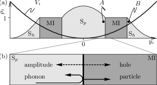
Figure 1: (a) One-dimensional model of a superfluid-Mott-insulator (S-MI) heterostructure in a trap defined by the potential $V_{i}$ at position $i$. The dark areas denote Mott-insulating regions with a fixed density $\rho_{i}$, while the bright areas are superfluids of condensed particles (center, S_p) and condensed holes (wings, S_h). (b) Sketch of a scattering event at the superfluid–Mott-insulator interface, where a phonon incident from the superfluid generates back-reflected quasi-particles of phonon- and amplitude-type as well as particle- and hole-type excitations transmitted into the Mott insulator.

Mesoscopic aspects in a wedding cake structure have been studied by Vishveshwara and Lannert, Vishveshwara and Lannert (2008) who calculated the Josephson coupling across a Mott-insulator domain (a S-MI-S junction) supported by the overlap between exponentially suppressed ground state wave functions (superfluid order parameters) across the Mott phase. Here, we are interested in the scattering dynamics of the excitations near a S-MI boundary and the transport associated with them across one or multiple interfaces; these excitations are sound (Goldstone) and massive (Higgs) modes within the superfluid phase, and particle- and hole-type excitations in the Mott insulator.Huber et al. (2007)

After developing the general framework describing transport in an inhomogeneous system with phase boundaries, we calculate analytically the reflection and transmission coefficients for a phonon mode of the superfluid incident on a Mott insulator [cf. Fig. 1(b)]. While these coefficients can be used to describe the scattering of a wave-packet of phonons (a density disturbance), here they mainly serve as an illustration of our approach. We then use our results (including those for scattering of massive modes) to calculate the heat transport through a Mott barrier. Knowledge of the heat conductivity $\kappa$ allows to estimate the thermal contact between superfluid shells in the wedding cake structure of a trapped Bose system. Note that temperature (actually entropy) imbalances quite naturally occur in optical lattice systems as the lattice potential is turned on and entropy is expelled from the newly formed Mott-insulating regions.Pollet et al. (2008) Our heat conductivity $\kappa$ then relates to the thermalization process across different superfluid rings.

Before developing our formalism in detail, we give an overview of the ideas and concepts utilized in this paper. The excitations close to one of the Mott-insulating lobes involve coherent superpositions of various site occupation numbers, and their wave functions are given by a four-spinor structure. This is reminiscent of the two-spinor structure of excitations in the Bogoliubov–de Gennes equations describing an inhomogeneous superconductor (note that for most unconventional superconductors, the reduction to a two-spinor is possible Honerkamp and Sigrist (1998)). The program to be carried out in order to find the transmission, reflection, and transformation of quasi-particles then is identical to the one introduced by Blonder, et al. Blonder et al. (1982) for the superconductor-normal-metal boundary (in order to simplify the analysis, we consider here a one-dimensional situation and leave geometric effects due to finite impact angles for a later study): First, we determine the excitation energies $\hbar\omega_{X}(k)$ and the four-spinor structure ${\bf X}(k)$ for the quasi-particle excitations in the superfluid (${\bf X}={\bf s},{\bf m}$: sound and massive modes) and in the Mott-insulator (${\bf X}={\bf p},{\bf h}$: particle and hole modes); below, this will be done for a translation invariant situation in a second-quantized formalism. Second, we switch to a first-quantized formulation and account for the inhomogeneous setup; for a slowly varying potential [$V_{i}\to V(y)$] this can be done within a quasi-classicalMigdal (1977) or Wentzel-Kramers-Brillouin (WKB) Wentzel (1926); Kramers (1926); Brillouin (1926) approximation, with the wave functions assuming the form

$$\boldsymbol{\psi}_{X}^{\epsilon}(y)=\frac{1}{\sqrt{|k_{X}^{\epsilon}(y)|}}\exp\Bigl{[}i\int^{y}dx\,k_{X}^{\epsilon}(x)\Bigr{]}{\bf X}[k_{X}^{\epsilon}(y)].$$ (1)

For a quasi-particle with energy $\epsilon$, the wave vector $k_{X}^{\epsilon}(y)$ is obtained via proper inversion of the dispersion $\hbar\omega_{X}(k)[V(y)]=\epsilon$, where the potential $V(y)$ enters the expression via a shift of the chemical potential, $\delta\mu\to\delta\mu-V(y)$. Third, we account for different phases in the setup by calculating the transfer matrix across the interface Azbel (1983) via matching of the wave functions and their derivatives at the boundary. For the case of a phonon incident from a (particle-type) superfluid S_p on a Mott-insulator MI [cf. Fig. 1(b)], the wave functions locally assume the form

$$\boldsymbol{\psi}_{\scriptscriptstyle\rm S}^{\epsilon}(y) =\boldsymbol{\psi}_{s}^{k_{s}^{\epsilon}}(y)+r_{\scriptscriptstyle\rm ss}\boldsymbol{\psi}_{s}^{-k_{s}^{\epsilon}}(y)+r_{ms}\boldsymbol{\psi}_{m}^{-k_{m}^{\epsilon}}(y),$$

$$\boldsymbol{\psi}_{\scriptscriptstyle\rm MI}^{\epsilon}(y) =\tau_{ps}\boldsymbol{\psi}_{p}^{k_{p}^{\epsilon}}(y)+\tau_{hs}\boldsymbol{\psi}_{h}^{k_{h}^{\epsilon}}(y),$$ (2)

with $\boldsymbol{\psi}_{X}^{\pm k}(y)$ denoting plane-wave functions of type (1) with constant wave vector $\pm k$. The scattering amplitudes $\tau_{ps}$ (transmitted particle), $\tau_{hs}$ (transmitted hole), $r_{ss}$ (reflected sound), and $r_{ms}$ (reflected massive mode) are obtained from the continuity conditions across the interface, $\boldsymbol{\psi}_{\scriptscriptstyle\rm S}^{\epsilon}(0)=\boldsymbol{\psi}_{\scriptscriptstyle\rm MI}^{\epsilon}(0)$ and $\partial_{y}\boldsymbol{\psi}_{\scriptscriptstyle\rm S}^{\epsilon}(0)=\partial_{y}\boldsymbol{\psi}_{\scriptscriptstyle\rm MI}^{\epsilon}(0)$.

In order to fully characterize the S_p-MI boundary, one has to determine the $4\times 4$ transfer matrix relating phonon and massive modes propagating to the left and right through the superfluid S_p with the particle and hole modes propagating to the left and right through the Mott-insulator, requiring the solution of four scattering problems of the above type [Eq. (2)] (the corresponding task has to be solved in order to describe the interface between a hole-type superfluid S_h and a Mott insulator). In the following, we concentrate exclusively on the scattering properties at the interface where the superfluid order parameter $\psi$ vanishes; this guarantees the solvability of the matching conditions at the boundary. As our final result, we present: (i) simple analytical expressions for the scattering coefficients at small hopping $t\to 0$ and near the critical value $t_{c}$ at the tip of the Mott-insulator lobe, as well as numerical results for two cases in between; and (ii) the behavior of the heat conductivity $\kappa$ as a function of the model parameters and the temperature $T$.

The body of the paper is organized as follows: In Sec. II, we derive the elementary excitations in the vicinity of the Mott-insulating regions of the Bose-Hubbard model. We briefly review the mapping to a spin-1 problem Huber et al. (2007) before discussing the spinor structure and symmetry properties of the wave functions. Section III is devoted to the calculation of the scattering coefficients for a superfluid-Mott-insulator interface, and the heat conductivity through a Mott barrier is determined in Sec. IV. We summarize our results and conclude in Sec. V.

II Excitations

In this section, we first derive the excitations of the strongly correlated superfluid and the Mott-insulating phase and exploit the time-reversal symmetry of the problem to obtain a well-suited set of spinor wave functions. For the reader who is less interested in the technical details, the energies $\hbar\omega_{X}(k)$ in Eqs. (4) and (5), the spinor wave functions ${\bf X}(k)$ in Eqs. (6) and (7), and their time-reversal invariant combinations [Eq. (12)], represent the main result of this section and Table 1 provides a physical interpretation of the four-spinor components.

We find the dispersion and eigenfunctions of quasiparticle excitations of the Bose Hubbard-model following the procedure described in detail in Ref. Huber et al., 2007. Starting with the Bose-Hubbard Hamiltonian (the bosonic operators $a_{i}$ create particles in Wannier states at site $i$, $\delta n_{i}=a_{i}^{{\dagger}}a_{i}-n_{0}$ measures the density from a mean density $n_{0}$, $t$ is the hopping energy, $U$ accounts for the on-site interaction, $\delta\mu$ is the chemical potential controlling the particle number, and $V_{i}$ accounts for the harmonic confinement),

$$H=-t\sum_{\langle i,j\rangle}a_{i}^{{\dagger}}a_{j}+\frac{U}{2}\sum_{i}(\delta n_{i})^{2}-\sum_{i}(\delta\mu-V_{i})\delta n_{i},$$ (3)

we first consider a homogeneous situation with $V_{i}\equiv 0$ and truncate the bosonic Hilbert space to a site basis with three local states $|0\rangle_{i}$, $|\!\pm\!1\rangle_{i}$. The state $|0\rangle_{i}$ refers to $n_{0}$ bosons on site $i$, while the states $|\!\pm\!1\rangle_{i}$ include one more (less) particle. Within this restricted space, we assume a trial wave function for the ground state $|\Psi\rangle=\prod_{i}|\psi_{i}\rangle$, where

$$|\psi_{i}\rangle=\cos(\vartheta)|0\rangle_{i}+\sin(\vartheta)\bigl{[}\sin(\chi)|\!+\!1\rangle_{i}+\cos(\chi)|\!-\!1\rangle_{i}\bigr{]}.$$

Minimizing the variational energy $\varepsilon_{\scriptscriptstyle\rm var}=\langle\Psi|H_{\scriptscriptstyle\rm BH}|\Psi\rangle$ with respect to $\sigma=\pi/4-\chi$ and subsequently expanding $\varepsilon_{\scriptscriptstyle\rm var}$ in the order parameter $\psi=\langle\Psi|a_{i}|\Psi\rangle=\sqrt{n_{0}/2}\sin(2\vartheta)$, we obtain $\varepsilon_{\scriptscriptstyle\rm var}\approx a\psi^{2}+b\psi^{4}/2$. To simplify expressions, we assume large filling with $\sqrt{n_{0}+1}\approx\sqrt{n_{0}}$. With the critical hopping $t_{c}=U/8n_{0}$, we find for the order parameter close to the upper (S_p-MI) and lower (S_h-MI) phase boundaries $\delta\mu_{c}^{\pm}=\pm U\sqrt{1-t/t_{c}}/2$ the result $|\psi|^{2}=\sqrt{1-t/t_{c}}\;\Delta^{\pm}_{\delta\mu}/t$, where $\Delta^{\pm}_{\delta\mu}=\delta\mu_{c}^{\pm}\pm\delta\mu$.

The calculation of the excitations above the mean-field ground state $|\Psi\rangle$ involves a spin-wave analysis in a slave boson description; the ground state in this effective pseudo-spin 1 formalism defines the direction of the magnetic order, while the remaining two degrees of freedom provide the excitations. For $\psi\to 0$, the result can be expressed as a $4\!\times\!4$ matrix Hamiltonian $H=\sum_{mn}T_{m}^{\dagger}{\cal H}_{mn}T_{n}$ with four-spinor operators ${\bf T}=(t_{1,k}^{{\dagger}},t_{-1,k}^{{\dagger}},t_{1,-k},t_{-1,-k})$ describing particle and hole creation and destruction above a mean-filling $n_{0}$ (cf. Table 1) (the operators $t_{\pm 1,i}^{\dagger}$ act on the vacuum states $|\mathrm{vac}\rangle_{i}$ and relate to the bosonic operators $a_{i}^{\dagger}$ via $t_{\pm 1,i}^{{\dagger}}=(a_{i}^{\dagger})^{n_{0}\pm 1}/\sqrt{(n_{0}\pm 1)!}$).

The diagonalization via a Bogoliubov transformation provides the dispersions (we measure wave vectors $k$ in units of $1/a$, with $a$ the lattice constant)

$$\hbar\omega_{p(h)}(k)=\frac{U}{2}\sqrt{1-(t/t_{c})\cos(k)}\mp\delta\mu$$ (4)

in the Mott-insulator and

$$\hbar\omega_{s(m)}(k)=4tn_{0}\sqrt{\alpha_{s(m)}^{2}-\beta_{s(m)}^{2}}\stackrel{{\scriptstyle k\rightarrow 0}}{{\approx}}\begin{cases}ck,\\ \Delta_{m}\end{cases}$$ (5)

in the superfluid phase for $\psi\rightarrow 0$ at $t<t_{c}$, where

$$\alpha_{s} = [2/(2-t/t_{c})-\cos(k)]/2,\qquad\alpha_{m}=2t_{c}/t+\alpha_{s},$$

$$\beta_{s} = -\beta_{m}=t\cos(k)/(2t_{c}-t).$$

The sound velocity $c$ of the phonon is $c=\sqrt{4Utn_{0}}$ $/(2t_{c}/t-1)$ and the gap $\Delta_{m}$ of the massive (or amplitude) mode is given by $\Delta_{m}=U\sqrt{1-t/t_{c}}$. At the S_p-MI interface, the particle excitation in the Mott-insulator transforms into the (particle-type) sound mode in S_p, while the hole excitation in the Mott-insulator transforms to the (hole-type) massive mode in S_p. Correspondingly, the bottom of the hole branch in the Mott-insulator matches up with the gap $\Delta_{m}$ of the massive (hole-type) mode in S_p, while the bottom of the particle branch in the Mott-insulator goes to zero. The use of Eq. (1) within an inhomogeneous superfluid phase requires generalization of the result in Eq. (5) to finite values of $\psi$, which provides the dependence on $\delta\mu$ away from $\delta\mu_{c}^{\pm}$ and hence on the local potential $V(y)$. Within the Mott region, the particle- and hole spectra undergo a simple shift $\pm\delta\mu$ [ cf. Eq. (4)], with a corresponding simple dependence on the smooth potential $V(y)$.

The spinor eigenstates in the Mott insulator are

$${\bf p}_{k}=\left\{\!\!\begin{array}[]{c}A(k)\\ 0\\ 0\\ B(k)\!\!\end{array}\!\!\right\}\qquad\mbox{and}\qquad{\bf h}_{k}=\left\{\!\!\begin{array}[]{c}0\\ -A(k)\\ -B(k)\\ 0\!\!\end{array}\!\!\right\},$$ (6)

with the coefficients

$$A(k) =\cosh({\rm atanh}\{(t/t_{c})\cos(k)/[2\!-\!(t/t_{c})\cos(k)]\}/2),$$

$$B(k) =\sinh({\rm atanh}\{(t/t_{c})\cos(k)/[2\!-\!(t/t_{c})\cos(k)]\}/2),$$

providing the “dressing” of a particle (with amplitude $A$ in ${\bf p}_{k}$) by missing hole-type fluctuations (with amplitude $B$) in the ground state (and vice versa for ${\bf h}_{k}$) and fulfill the normalization condition.

four-spinor	Microscopic interpretation	Dirac
$\left\{\!\!\begin{array}[]{c}t_{1,k}^{{\dagger}}\\ t_{-1,k}^{{\dagger}}\\ t_{1,-k}\\ t_{-1,-k}\phantom{,}\!\!\end{array}\!\!\right\}$	$\begin{array}[]{l}\mbox{create particle}\\ \mbox{create hole}\\ \mbox{destroy particle fluctuation in gs}\\ \mbox{destroy hole fluctuation in gs}\end{array}$	$\begin{array}[]{l}\mbox{$e^{-}$, $\uparrow$}\\ \mbox{$e^{-}$, $\downarrow$}\\ \mbox{$e^{+}$, $\uparrow$}\\ \mbox{$e^{+}$, $\downarrow$}\end{array}$

Table 1: Physical interpretation of the four-spinor and its similarity to the Dirac spinor. In both cases, we deal with two species of “particles”: the particle and hole excitations discussed here correspond to spin-up/down electrons in the Dirac equation. The role of anti-particles in the Dirac spinor is played by ground state fluctuations in the present context: the anti-particle of a particle is a fluctuation with a “missing” particle in the gs and similar for the hole. Hence the top and bottom entries are both particle-type (creation of particle and destruction of a hole), while the two middle entries are both hole-type (creation of a hole and destruction of a particle).

The spinor eigenstates in the particle-condensed superfluid phase S_p are

$${\bf s}_{k}^{\scriptscriptstyle\rm p}=\left\{\!\!\begin{array}[]{c}-\Omega_{+}A_{s}(k)\\ \Omega_{-}A_{s}(k)\\ -\Omega_{+}B_{s}(k)\\ \Omega_{-}B_{s}(k)\!\!\end{array}\!\!\right\}\quad\mbox{and}\quad{\bf m}_{k}^{\scriptscriptstyle\rm p}=\left\{\!\!\begin{array}[]{c}\Omega_{-}A_{m}(k)\\ \Omega_{+}A_{m}(k)\\ \Omega_{-}B_{m}(k)\\ \Omega_{+}B_{m}(k)\!\!\end{array}\!\!\right\},$$ (7)

with the coefficients

$$A_{s(m)} =\cosh\{{\rm atanh}[\beta_{s(m)}(k)/\alpha_{s(m)}(k)]/2\},$$ (8)

$$B_{s(m)} =\sinh\{{\rm atanh}[\beta_{s(m)}(k)/\alpha_{s(m)}(k)]/2\}.$$ (9)

Furthermore, $\Omega_{\pm}=[\cos(f(t))\pm\sin(f(t))]/\sqrt{2}$ with $f(t)=\arctan[2(t_{c}/t)\sqrt{1-t/t_{c}}]$. The eigenstates for S_h are obtained by replacing

$$\Omega_{+}\leftrightarrow\Omega_{-}.$$ (10)

The nature of these excitations is easily understood in the limits $t\to 0$ and $t\to t_{c}$. For $t\to 0$, the coefficients $A,A_{s(m)}\to 1$ and $B,B_{s(m)}\to 0$, telling us that the ground state turns into a classical one devoid of fluctuations [cf. Table 1]. The excitations [Eq. (6)] in the Mott phase combine particles with absent hole fluctuations and holes with absent particle fluctuations and hence are of particle and hole types, respectively. With $\Omega_{+}\to 1$ and $\Omega_{-}\to 0$ the weights are set differently in the superfluid phase; here, the excitations involve particles dressed with holes and holes dressed with particles, reflecting the collective nature of these excitations. Crossing the boundary $\delta\mu^{+}_{c}$ into the particle-type superfluid S_p, the particle mode of the Mott insulator condenses, imprinting the predominant particle nature onto the sound mode [the gapped hole mode goes over to the massive (amplitude) mode in the superfluid].

For $t\to t_{c}$, the coefficients $A,A_{s(m)}\to\infty$ and $B,B_{s(m)}\to\infty$; the excitations exploit the strong fluctuations in the ground state but keep their particle and hole character in the Mott insulator. With $\Omega_{\pm}\to 1/\sqrt{2}$, both sound and massive modes have a mixed particle-hole character and draw large weights from the ground-state fluctuations.

In the next section, we will have to match the spinor wave functions and their derivatives, providing us with eight conditions for only four unknown scattering coefficients. In order to eliminate the additional spurious conditions, it is convenient to exploit the symmetry under time reversal and we introduce the time-reversal operator

$${\mathcal{T}}={\mathcal{C}}\begin{pmatrix}0&\sigma_{0}\\ \sigma_{0}&0\end{pmatrix},$$ (11)

where $\mathcal{C}$ denotes the action of complex conjugation and $\sigma_{0}$ is the identity matrix in two dimensions. The form of ${\mathcal{T}}$ can be inferred from the behavior of $a_{i}$ under time reversal and the relations between the operators $a_{i}$ and $t_{i,0},t_{i,\pm 1}$. In addition to the above spinors ${\bf X}={\bf p},{\bf h},{\bf s},{\bf m}$, we define the four linearly independent eigenvectors ${\mathcal{T}}{\bf X}$. For the situation with unbroken ${\mathcal{T}}$ invariance discussed here,not (a) it is convenient to define the new states,

$${\bf X}_{k}^{\pm}=({\bf X}_{k}\mp i{\mathcal{T}}{\bf X}_{k})/\sqrt{2}.$$ (12)

These form a basis of ${\mathcal{T}}$ representations and are multiplied with $\pm i$ under the operation ${\mathcal{T}}$. Without loss of generality, we choose to work with the “+”-eigenstates and drop the superscript in the following.

With these spinors at hand, we are now in the position to describe inhomogeneities. For piecewise constant “potentials”, we can use plane-wave-type left and right moving spinor wave functions

$$\boldsymbol{\psi}_{X}^{\pm k_{X}^{\epsilon}}(y)=e^{i(\pi\mp\pi)/4}e^{\pm ik_{X}^{\epsilon}y}{\bf X}_{k_{X}^{\epsilon}},$$ (13)

and combine them into the scattering states defined in Eq. (2). For slowly varying parameters (“potentials”), the states [Eq. (12)] determine the spinor structure in Eq. (1).

III Scattering coefficients

Next, we discuss a specific situation, the scattering of a phonon on a Mott-insulator boundary, and determine the scattering coefficients by matching the wave functions [Eq. (2)] at the boundary between the superfluid and the insulating region. The scattering state (2) describes a phonon excitation incident from a particle-type superfluid S_p onto a Mott insulator [cf. Fig. 1]. These excitations are relevant in an experiment where a density perturbation is applied to the middle of the trap;Kollath et al. (2005) while one has to describe the density perturbation by a wave packet of phonons, here, we only discuss the scattering properties of plane-wave excitations as the generic building block. Imposing the continuity conditions across the S_p-MI interface, we obtain the scattering coefficients $r_{ss}$, $r_{ms}$, $\tau_{ps}$, and $\tau_{hs}$; only the first two spinor elements are relevant as the second two satisfy the matching conditions automatically due to ${\mathcal{T}}$ invariance. In the following, we discuss these coefficients in the limiting cases $t\to 0,~{}t_{c}$ and illustrate their behavior at intermediate values of $t$ in Fig. 2. Furthermore, here, we restrict the discussion to those modes propagating in the superfluid as well as in the Mott-insulator region; in the next section, where the heat transport through a finite Mott region is discussed, the contribution of evanescent modes has to be considered as well.

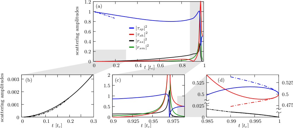
Figure 2: Scattering coefficients for an incoming sound mode at an energy $\epsilon=\hbar\omega_{s}(\pi)/4$. (a) For all values of $t/t_{c}$. The full lines show the exact values, while the dash-dotted line is the approximate value from Eq. (14). (b) Comparison between the exact and approximate values for $r_{ss}$. (c) All coefficients around the “critical” value $t\approx 0.971$ where for $\epsilon=\hbar\omega_{s}(\pi)/4$ the hole and massive modes become exponentially damped. Note, that values of the scattering coefficients larger than 1 are not in contradiction with particle conservation as these excitations do not have a well defined particle character. (d) For values $t\approx t_{c}$ the dash-dotted results from Eq. (16) again describe the exact solutions well.

For $t\to 0$, a sound mode incident from S_p can be reflected as a sound mode or transmitted into the Mott insulator as a particle excitation; hence. the coefficients connecting to propagating scattered modes are $r_{ss}$ and $\tau_{ps}$; given the energy $\epsilon$ of the incident phonon mode, they can be conveniently expressed through the wave vectors $k_{s}^{\epsilon}$ and $k_{p}^{\epsilon}$ of the sound- and particle excitations involved,

$$r_{ss}(\epsilon) \approx i\frac{k_{p}^{\epsilon}-k_{s}^{\epsilon}}{k_{s}^{\epsilon}+k_{p}^{\epsilon}}+{\mathcal{O}}[(t/t_{c})^{2}],$$ (14)

$$\tau_{ps}(\epsilon) \approx-\frac{2k_{s}^{\epsilon}}{k_{s}^{\epsilon}+k_{p}^{\epsilon}}\biggl{(}1-\frac{t}{4t_{c}}\frac{\cos(k_{s}^{\epsilon})}{1-\cos(k_{s}^{\epsilon})}\biggr{)}+{\mathcal{O}}[(t/t_{c})^{2}]$$

(the coefficients $r_{ms}$ and $\tau_{hs}$ describe scattering into evanescent modes). To leading order in $t/t_{c}$, we recognize the standard expressions for the one-dimensional barrier problem where the reflection and transmission amplitudes can be expressed in terms of momentum ratios. This result comes about since, for $t=0$, the two phases, S_p and the Mott insulator, are essentially identical. However, for the current setup, the height of the “barrier” is not a free parameter due to the generic nature of the interface; the result then is determined by the dispersions at the boundary. For a small but finite hopping $t/t_{c}$, the Mott insulator remains essentially unchanged, while the bosons in the superfluid exploit the kinetic energy. This leads to a reduced transmission due to the wave function mismatch at the boundary, as reflected by the term $\!\propto t/t_{c}$ in $\tau_{ps}$.

Next, we discuss the situation near the tip of the Mott lobe; in order to formulate the results for $t\to t_{c}$, we first define the reduced distance $\delta_{t}=1-t/t_{c}>0$ from the tip of the Mott lobe and the coherence functions

$$f_{\pm}(k)=[A(k)\pm iB(k)]\big{|}_{t=t_{c}}.$$ (15)

While the phases $\arg[f_{\pm}(k)]$ run from $\arg[f_{\pm}(0)]=\mp\pi/4$ to $\arg[f_{\pm}(\pi)]=\pm{\rm acos}(1/\sqrt{3}+1/\sqrt{6})$, both moduli diverge at $k\to 0$, reflecting the softening of all modes at the tip of the Mott lobe; however, the ratio $|f_{+}(k)/f_{-}(k)|^{2}\equiv 1$ remains finite. Away from $k\rightarrow 0$ the moduli of $f_{\pm}(k)$ are well behaved. To leading order in $\delta_{t}$ we obtain

$$r_{ss}(\epsilon) \approx i\frac{k_{p}^{\epsilon}-k_{s}^{\epsilon}}{k_{p}^{\epsilon}+k_{s}^{\epsilon}}+{\mathcal{O}}(\delta_{t}),\qquad r_{ms}(\epsilon)\approx{\mathcal{O}}(\delta_{t}),$$ (16)

$$\tau_{ps}(\epsilon) \approx-\frac{\sqrt{2}k_{s}^{\epsilon}}{k_{p}^{\epsilon}+k_{s}^{\epsilon}}\biggl{(}\frac{f_{-}(k_{s}^{\epsilon})}{f_{+}(k_{p}^{\epsilon})}+\frac{f_{-}(k_{s}^{\epsilon})}{f_{-}(k_{p}^{\epsilon})}\sqrt{\delta_{t}}\biggr{)}+{\mathcal{O}}(\delta_{t}),$$

$$\tau_{hs}(\epsilon) \approx-\frac{\sqrt{2}k_{s}^{\epsilon}}{k_{h}^{\epsilon}+k_{s}^{\epsilon}}\biggl{(}\frac{f_{-}(k_{s}^{\epsilon})}{f_{+}(k_{h}^{\epsilon})}-\frac{f_{-}(k_{s}^{\epsilon})}{f_{-}(k_{h}^{\epsilon})}\sqrt{\delta_{t}}\biggr{)}+{\mathcal{O}}(\delta_{t}).$$

For $\delta_{t}\to 0$, we have $k_{s}^{\epsilon}\approx k_{h}^{\epsilon}\approx k_{p}^{\epsilon}$, the coherence factors are approximately unity, and we again recognize the typical result for a simple barrier. This time, however, the particle and the hole branches are degenerate and are transmitted equally to leading order, explaining the factor $\sqrt{2}$. Furthermore, the massive mode is orthogonal to the sound mode and does not contribute in leading order. Going to nonzero $\delta_{t}$, the superfluid develops “particle” nature, leading to an increase (reduction) in $\tau_{ps}$ ($\tau_{hs}$).

The behavior of the scattering coefficients for intermediate values of $t/t_{c}$ is shown in Fig. 2. The coefficients are given for an energy $\epsilon=\hbar\omega_{s}(\pi)/4$ allowing for a comparison at different values of $t/t_{c}$. Note that for this energy, the hole and massive modes become non-propagating for $t/t_{c}\lesssim 0.971$. The corresponding density of states effect is responsible for the irregular behavior around $t/t_{c}\approx 0.971$. At small $t/t_{c}$, the approximations [Eq. (14)] are in good agreement with the exact values; the same is true near the tip of the Mott lobe, where the coefficients [Eq. (16)] agree well with the exact numerical values. Here, however, the close vicinity of the point where the massive mode and the hole turn evanescent spoils the applicability of the analytical results much faster.

Given the results above, we note the following generic trends: Scattering coefficients relating modes of equal type, e.g., particle-type sound in the S_p and particle excitations in the Mott insulator are large, while scattering between unequal modes, e.g., particle-type sound in the S_p and hole excitations in the Mott insulator is suppressed. Furthermore, the energy-dependent point on the $t/t_{c}$ axis where the massive and hole modes turn evanescent controls the breakdown of the approximate formulas (14) and (16). The same statements hold for the respective cases of an incoming massive mode and the inverted situations at the lower boundary of the Mott lobe, i.e., with initial states in S_h.

IV Heat conductivity

As an application, we calculate the transport of heat through a Mott-insulating layer within a wedding cake structure. The derived heat conductivity $\kappa$ provides insight into the thermalization process when the lattice potential is ramped up,Pollet et al. (2008) and quantifies to what extent two superfluid shells are in thermal contact through the Mott layer. In order to calculate $\kappa$, we consider the heat currentMahan (1990)

$${\bf Q}_{E}=\sum_{\alpha,\beta}\int d\epsilon\,N_{\alpha}(\epsilon){\bf v}_{\beta}(\epsilon)\epsilon g(\epsilon,T)|\tau_{\alpha\beta}|^{2},$$ (17)

where the sum is running over input ($\alpha$) and output ($\beta$) channels. In Eq. (17), $N_{\alpha}(\epsilon)$ is the density of states in the input channels $\alpha$, ${\bf v}_{\beta}(\epsilon)$ is the velocity associated with the excitations at energy $\epsilon$ in the output channels $\beta$, and we integrate over all energies $\epsilon$. The Bose-Einstein distribution $g(\epsilon,T)=[\exp(\epsilon/k_{\scriptscriptstyle\rm B}T)-1]^{-1}$ controls the occupation of the bosonic modes and $\tau_{\alpha\beta}$ are the transmission amplitudes connecting input and output channels. The linear-response expression Eq. (17) describes the situation close to equilibrium. In a real experiment, the initial state after ramping of the optical potential may be far away from the bosonic equilibrium distribution $g(\epsilon,T)$. Nevertheless, the calculation of the linear-response result [Eq. (17)] provides some generic insights into the behavior of the system which applies to such a situation as well.

It is instructive to calculate the maximal heat conductivity of a homogeneous Mott region. For temperatures higher than all energy scales in the problem (the repulsion $U$), but lower than the band gap to the next Bloch band, the heat conductivity is finite and given by

$$\kappa_{\infty}^{\scriptscriptstyle\rm hom} =\sum_{\alpha=p,h}\int_{0}^{\pi/a}\!\!\frac{dk}{\pi/a}\,v_{\alpha}(k)\hbar\omega_{\alpha}(k)\partial_{T}g(\epsilon,T\gg U)$$

$$=\frac{Ua}{\hbar}k_{\scriptscriptstyle\rm B}\biggl{(}\sqrt{1+t/t_{c}}-\sqrt{1-t/t_{c}}\biggr{)},$$ (18)

where we explicitly accounted for the lattice constant $a$. From Eq. (18) we learn that the coefficient $\kappa$ describes the transport of entropy “$k_{\scriptscriptstyle\rm B}$” with velocity $Ua/\hbar$. Below, we take

$$\kappa_{\scriptscriptstyle\rm ref}=\kappa_{\infty}^{\scriptscriptstyle\rm hom}(t\rightarrow t_{c})=\sqrt{2}\frac{Ua}{\hbar}k_{\scriptscriptstyle\rm B}$$ (19)

as our reference value for the heat conductivity.

We calculate the heat current [Eq. (17)] from one superfluid shell, point $A$ in Fig. 1(a), to point $B$ in the next shell and take the derivative with respect to the temperature $T$ to obtain $\kappa(T)$ (cf. Fig 5). The input channels $\alpha$ are given by the phonons and massive particles impinging onto the Mott insulating phase at point $A$, i.e., from the particle-like superfluid S_p. The output channels on the other side of the insulating region are the corresponding modes in S_h.

To obtain the transmission amplitudes $\tau_{\alpha\beta}$, we apply a transfer matrix formalismAzbel (1983) to divide the problem into three parts, the scattering across the interface between the superfluid S_p and the Mott region, point $A$ in Fig. 1(a), the propagation within the Mott layer, and the scattering at the second interface connecting the Mott insulator and the superfluid S_h [cf. point $B$ in Fig. 1(a)]. The scattering at the two interfaces is handled as described in Sec. III above; in addition, scattering amplitudes into and from evanescent modes now have to be accounted for.

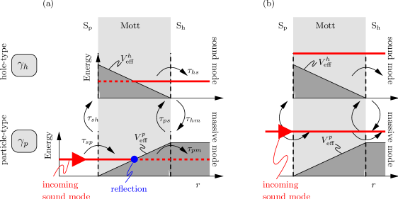
Figure 3: Sketch of a scattering event of an incoming phonon from S_p. (a) The incident sound mode is transformed into a particle and a hole with amplitudes $\tau_{sp}$ and $\tau_{sh}$, respectively. Inside the Mott layer, the particle propagates until it hits the potential, where it is either reflected or tunnels under the barrier. The hole emerges from under the barrier and propagates to the other end of the layer. At the boundary to S_h, both modes are converted into the modes of the superfluid with the corresponding amplitudes. (b) The same situation with a higher energy of the incoming sound mode that allows for undamped propagation through the Mott region.

To describe the transfer from the superfluid phase into the Mott insulator and vice versa, we match the wave functions [Eq. (13)] and their derivatives at the boundary (placed at $y=0$): we define the wave functions

$$\boldsymbol{\psi}_{\scriptscriptstyle\rm MI}(y)\! =\!P_{r}\boldsymbol{\psi}_{p}^{k}(y)\!+\!P_{l}\boldsymbol{\psi}_{p}^{\!-k}(y)\!+\!H_{r}\boldsymbol{\psi}_{h}^{k}(y)\!+\!H_{l}\boldsymbol{\psi}_{h}^{\!-k}(y),$$

$$\boldsymbol{\psi}_{\scriptscriptstyle\rm S}(y)\! =\!S_{r}\boldsymbol{\psi}_{s}^{k}(y)\!+\!S_{l}\boldsymbol{\psi}_{s}^{\!-k}(y)\!+\!M_{r}\boldsymbol{\psi}_{m}^{k}(y)\!+\!M_{l}\boldsymbol{\psi}_{m}^{\!-k}(y),$$

and impose the matching conditions $\boldsymbol{\psi}_{\scriptscriptstyle\rm MI}(0)=\boldsymbol{\psi}_{\scriptscriptstyle\rm S}(0)$ and $\partial_{y}\boldsymbol{\psi}_{\scriptscriptstyle\rm MI}(0)=\partial_{y}\boldsymbol{\psi}_{\scriptscriptstyle\rm S}(0)$ for the two first components; the conditions for the other two components then are fulfilled automatically due to ${\mathcal{T}}$-symmetry. The subscripts $l$ and $r$ denote right- and left-moving excitations, respectively. This procedure provides us with four relations connecting the four amplitudes on one side of the interface with the four on the other. Solving for the coefficients $P_{l(r)}$ and $H_{l(r)}$, we obtain the transfer matrix $\mathsf{M}_{\scriptscriptstyle\rm S-MI}$ defined as

$$\begin{pmatrix}P_{r}\\ P_{l}\\ H_{r}\\ H_{l}\end{pmatrix}=\mathsf{M}_{\scriptscriptstyle\rm S-MI}\begin{pmatrix}S_{r}\\ S_{l}\\ M_{r}\\ M_{l}\end{pmatrix}.$$ (20)

This transfer matrix depends on the type of interface, S_p or S_h, connecting to the Mott layer; correspondingly, we denote the two different matrices by $\mathsf{M}_{\scriptscriptstyle\rm S-MI}^{\scriptscriptstyle\rm p(h)}$. Note that the four-dimensional character of Eq. (20) is due to the restriction to the “$+$”-sector of $\mathcal{T}$; in general, one expects the transfer matrix to act on a vector space of twice the dimension of the spinor. However, the matrix elements connecting the two sectors “$+$” and “$-$” vanish for a $\mathcal{T}$-symmetric system.

The new task to analyze is the propagation of particle- and hole excitations through the Mott region $0<y<L$ as described by the transfer matrix

$$\begin{pmatrix}P_{r}(y=L)\\ P_{l}(y=L)\\ H_{r}(y=L)\\ H_{l}(y=L)\end{pmatrix}=\mathsf{M}_{\scriptscriptstyle\rm MI}\begin{pmatrix}P_{r}(y=0)\\ P_{l}(y=0)\\ H_{r}(y=0)\\ H_{l}(y=0)\end{pmatrix}.$$ (21)

This task requires the evaluation of the WKB-phases (between arbitrary points $a$ and $b$)

$$\varphi^{p(h)}_{a,b}=\int_{a}^{b}dx\,k_{p(h)}^{\epsilon}(x)$$ (22)

of Eq. (1) in the presence of an inhomogeneous potential $V(y)$. Attention has to be paied to properly treat the classical turning points where the quasi-classical approximation [Eq. (1)] breaks down; Fig. 3 illustrates typical situations in the present context, where particles and holes incident from the left are stopped by the potential $V_{\scriptscriptstyle\rm eff}^{p(h)}$ and turn evanescent or tunnel as evanescent modes into the MI and turn into propagating modes at the right of the Mott region. Such turning points are dealt with in the standard wayMigdal (1977) and lead to additional scattering phases $\pm\pi/4$ in the propagator.

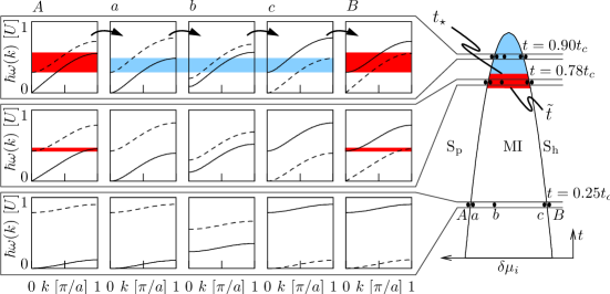
Figure 4: (color online) Left: sketch of the local excitation spectra at different points $A,a,b,c,B$ (columns) in the inhomogeneous system for three different values of the hopping amplitude at $t/t_{c}=0.9,0.78,0.25$ (rows); Hole-like spectra are dashed; particle-like spectra are solid lines. Right: local phase diagram with Mott insulating and superfluid regions depending on the chemical potential $\delta\mu_{i}$ and the hopping $t/t_{c}$. The blue (light gray) shaded area of the Mott lobe corresponds to values of $t/t_{c}$ for which the hole at point $a$ has spectral overlap with the hole-like spectra at $c$, allowing for undamped propagation in the energy window given in blue (light gray) on the left. The red (dark gray) shaded area of the Mott lobe marks values of $t$ for which the modes in the superfluid have mutual spectral overlap for an non-vanishing range of energy as shown on the left. For values $t<\tilde{t}$, the crossed terms do not contribute (phonon $\leftrightarrow$ massive mode) to the heat conductivity (see text).

Depending on the appearance of turning points in the particle and/or hole channel, the transfer matrix $M_{{\scriptscriptstyle\rm MI}}$ assumes different forms. The simplest case is realized near the tip of the Mott lobe, where particle and hole modes can propagate unhindered through the Mott region [cf. Fig. 4]. In this case, the matrix is diagonal and multiplies each component of the four-spinor with appropriate phase factors,

$$\mathsf{M}_{{\scriptscriptstyle\rm MI}}=\begin{pmatrix}e^{i\varphi_{0,L}^{p}}&0&0&0\\ 0&e^{-i\varphi_{0,L}^{p}}&0&0\\ 0&0&e^{i\varphi_{0,L}^{h}}&0\\ 0&0&0&e^{-i\varphi_{0,L}^{h}}\end{pmatrix}=\begin{pmatrix}\mathsf{m}_{\scriptscriptstyle\rm MI}^{p}&0\\ 0&\mathsf{m}_{\scriptscriptstyle\rm MI}^{h}\end{pmatrix}.$$

The appearance of a turning point in the particle (hole) channel renders the $2\times 2$ block matrix $\mathsf{m}_{{\scriptscriptstyle\rm MI}}^{p}$ ($\mathsf{m}_{{\scriptscriptstyle\rm MI}}^{h}$) describing particle (hole) propagation non-diagonal; note that particles (holes) then are reflected but never converted into one another. Assuming a classical turning point at $r_{\scriptscriptstyle\rm cl}$ (cf. trajectory $\gamma_{p}$ in Fig. 3), the transfer matrix for a particle excitation assumes the form

$$\mathsf{m}_{{\scriptscriptstyle\rm MI}}^{p}=\begin{pmatrix}\frac{1}{2}e^{i\varphi_{0,L}^{p}-i\pi/4}&\frac{1}{2}e^{-i\varphi_{0,r_{\scriptscriptstyle\rm cl}}^{p}+i\varphi_{r_{\scriptscriptstyle\rm cl},L}^{p}+i\pi/4}\\ e^{i\varphi_{0,r_{\scriptscriptstyle\rm cl}}^{p}-i\varphi_{r_{\scriptscriptstyle\rm cl},L}^{p}+i\pi/4}&e^{-i\varphi_{0,L}^{p}-i\pi/4}\end{pmatrix}.$$

The equivalent expression for the hole excitation (trajectory $\gamma_{h}$ in Fig. 3), reads as

$$\mathsf{m}_{{\scriptscriptstyle\rm MI}}^{h}=\begin{pmatrix}e^{i\varphi_{0,L}^{h}+i\pi/4}&\frac{1}{2}e^{-i\varphi_{0,r_{\scriptscriptstyle\rm cl}}^{h}+i\varphi_{r_{\scriptscriptstyle\rm cl},L}^{h}-i\pi/4}\\ e^{i\varphi_{0,r_{\scriptscriptstyle\rm cl}}^{h}-i\varphi_{r_{\scriptscriptstyle\rm cl},L}^{h}-i\pi/4}&\frac{1}{2}e^{-i\varphi_{0,L}^{h}+i\pi/4}\end{pmatrix}.$$

Note, that due to particle-hole symmetry, the turning points $r_{\scriptscriptstyle\rm cl}$ are the same for particles and holes. The “phases” $\varphi_{a,b}^{p(h)}$ have to be calculated numerically. The total transfer matrix, connecting the two superfluids on either side of the Mott insulator, is given by

$$\mathsf{M}_{\scriptscriptstyle\rm tot}=(\mathsf{M}_{\scriptscriptstyle\rm S-MI}^{\scriptscriptstyle\rm h})^{-1}\mathsf{M}_{\scriptscriptstyle\rm MI}\mathsf{M}_{\scriptscriptstyle\rm S-MI}^{\scriptscriptstyle\rm p}.$$ (23)

We obtain the scattering matrix $\mathsf{S}$ by solving the linear equation

$$\begin{pmatrix}S_{\scriptscriptstyle\rm out}^{\scriptscriptstyle\rm h}\\ S_{\scriptscriptstyle\rm in}^{\scriptscriptstyle\rm h}\\ M_{\scriptscriptstyle\rm out}^{\scriptscriptstyle\rm h}\\ M_{\scriptscriptstyle\rm in}^{\scriptscriptstyle\rm h}\\ \end{pmatrix}=\mathsf{M}_{\scriptscriptstyle\rm tot}\begin{pmatrix}S_{\scriptscriptstyle\rm in}^{\scriptscriptstyle\rm p}\\ S_{\scriptscriptstyle\rm out}^{\scriptscriptstyle\rm p}\\ M_{\scriptscriptstyle\rm in}^{\scriptscriptstyle\rm p}\\ M_{\scriptscriptstyle\rm out}^{\scriptscriptstyle\rm p}\\ \end{pmatrix}$$ (24)

for the amplitudes of the outgoing excitations $S_{\scriptscriptstyle\rm out}^{\scriptscriptstyle\rm p}$, $M_{\scriptscriptstyle\rm out}^{\scriptscriptstyle\rm p}$, $S_{\scriptscriptstyle\rm out}^{\scriptscriptstyle\rm h}$, and $M_{\scriptscriptstyle\rm out}^{\scriptscriptstyle\rm h}$. For the heat conductivity, we are only interested in the transmission amplitudes connecting the channels of incoming phonons and massive modes from S_p to the outgoing excitations in S_h. Within this subspace the scattering matrix reads as

$$\begin{pmatrix}S_{\scriptscriptstyle\rm out}^{\scriptscriptstyle\rm h}\\ M_{\scriptscriptstyle\rm out}^{\scriptscriptstyle\rm h}\end{pmatrix}=\mathsf{S}\begin{pmatrix}S_{\scriptscriptstyle\rm in}^{\scriptscriptstyle\rm p}\\ M_{\scriptscriptstyle\rm in}^{\scriptscriptstyle\rm p}\end{pmatrix}=\begin{pmatrix}\tau_{ss}&\tau_{sm}\\ \tau_{ms}&\tau_{mm}\end{pmatrix}\begin{pmatrix}S_{\scriptscriptstyle\rm in}^{\scriptscriptstyle\rm p}\\ M_{\scriptscriptstyle\rm in}^{\scriptscriptstyle\rm p}\end{pmatrix},$$ (25)

and provides us with the explicit form of the scattering amplitudes $\tau_{\alpha\beta}$ appearing in the expression for the heat current [Eq. (17)].

The density of states $N_{\alpha}(\epsilon)$ and velocity $v_{\beta}(\epsilon)$ derive from the dispersion relations $\omega_{s(m)}$ in Eq. (5). In one dimension, these quantities are related via $v_{s(m)}=1/N_{s(m)}(\epsilon)$ and hence only in processes where the phonon and massive mode channels are mixed with $\alpha\neq\beta$; there appears a ratio $N_{s(m)}(\epsilon)/N_{m(s)}(\epsilon)$, otherwise all density of states effects cancel out.

Next, we identify those regions in the Mott lobe where we expect a large value of $\kappa$. Figure 4 shows the evolution of the spectra upon crossing the Mott-insulating region, starting with sound- and massive modes in the particle-type superfluid S_p at point $A$ right at the interface, the swap of particle- and hole-type branches within the MI regime with a potential rising approximately linearly with distance; see diagrams “a”, “b”, and “c” in Fig. 4, and the interchanged massive- and sound modes in the hole-type superfluid S_p at point $B$, again right at the interface. Following the evolution of the spectra from the tip of the Mott lobe at $t=t_{c}$ down to $t=0$, various regimes can be identified where transport is favored, either via full propagation through the Mott region or via conservation of the particle/hole nature of the excitation along the trajectory. At large values of $t$ close to the tip of the lobe an appreciable part of the particle- and hole branches overlaps, allowing these excitations to propagate through the Mott insulating without damping. This overlap terminates when the bottom of the hole band lines up with the top of the particle band [$\hbar\omega_{p}(\pi/a)=\hbar\omega_{h}(0)$; cf. Eq. (4) and diagram “a” in Fig. 4], defining the special value $t_{\ast}=(4/5)t_{c}$. Another relevant point is $\tilde{t}$, where the massive and sound modes stop overlapping in the superfluid; see diagram “$A$” in Fig. 4. Comparing the bottom of the massive mode at $k=0$ with the top of the sound mode at $k=\pi$, we find that this overlap persists as long as $t>\tilde{t}$ with $\tilde{t}=(3-\sqrt{5})t_{c}$; and we have $\Delta_{m}<W_{\varphi}$, where $W_{s}=\hbar\omega_{s}(\pi/a)$ denotes the width of the sound mode in S_p. In this situation, the particle-type modes in the left (sound) and right (massive) superfluids overlap (and vice versa for the hole modes) and large transmissions at the boundaries enhance the contribution of these modes to $\kappa$. Finally, for $t<\tilde{t}$, propagation through the Mott region is always damped and excitations have to be converted between particle- and hole-types, hence only direct terms $\propto|\tau_{ss}|^{2}$ (particle-type sound is converted to hole-type sound) and $\propto|\tau_{mm}|^{2}$ (hole-type Higgs is converted to particle-type Higgs) contribute. Accordingly, the heat conductivity $\kappa$ naturally splits into direct and cross terms, with the latter ones contributing with large weight but only for $t>\tilde{t}$ where $W_{s}>\Delta_{m}$,

$$\kappa(T)=\kappa_{\scriptscriptstyle\rm dir}(T)+\Theta(W_{s}-\Delta_{m})\kappa_{\scriptscriptstyle\rm cross}(T),$$ (26)

with

$$\kappa_{\scriptscriptstyle\rm dir} =\int_{0}^{W_{\varphi}}\!\!\!\!\!\!\!d\epsilon\,\epsilon|\tau_{ss}|^{2}\frac{\partial g}{\partial T}+\int_{\Delta_{m}}^{W_{m}}\!\!\!\!\!\!\!d\epsilon\,\epsilon|\tau_{mm}|^{2}\frac{\partial g}{\partial T},$$ (27)

$$\kappa_{\scriptscriptstyle\rm cross} =\int_{\Delta_{m}}^{W_{\varphi}}\!\!\!\!\!\!\!d\epsilon\,\epsilon\biggl{[}\frac{N_{s}(\epsilon)}{N_{m}(\epsilon)}|\tau_{ms}|^{2}+\frac{N_{m}(\epsilon)}{N_{s}(\epsilon)}|\tau_{sm}|^{2}\biggr{]}\frac{\partial g}{\partial T}.$$ (28)

For the direct terms, the initial and the final states are both sound modes or both massive modes and the density of states cancels against the velocity factor.

The expressions in Eqs. (27) and (28) have to be calculated numerically and provide the final result for the heat conductivity $\kappa(T)$ shown in Fig. 5 as a function of $T/U$ for different values of $t/t_{c}$. The overall shape involves an exponential suppression at small temperatures $T$, hinting to the presence of an effective gap $\Delta_{\scriptscriptstyle\rm eff}$, and a saturation value $\kappa_{\infty}$ at large temperatures when all modes within the finite bandwidth contribute to the transport. Furthermore, the transport efficiency decreases with decreasing $t$, as is to be expected on the basis of the above analysis; cf. Fig. 4.

Figure 5: (a) Heat conductivity $\kappa(T)$ for different values of $t$ ($t=0.9,0.82,0.78,0.74t_{c}$, from the back to the front) for a Mott layer of thickness $L_{0}=10a$ at $t=0$ ($a$ denotes the lattice constant). The structure of $\kappa(T)$ for small $T$ is dictated by the spectral gap in the intermediate Mott region. For smaller values of $t$, where only damped modes contribute to transport, the heat conductivity is exponentially suppressed and not shown here. (b) The dependence of the maximal heat conductivity $\kappa_{\infty}=\kappa(T\gg U/k_{\scriptscriptstyle\rm B})$ on the hopping amplitude $t$ displaying the qualitative change for $t<\tilde{t}$ in the plot, where the strong suppression sets in. The change at $t_{\star}$ is masked by a scattering resonance in the intermediate $\tilde{t}<t<t_{\star}$ regime.

Given the complexity of the result expressed through Eqs. (27) and (28) and the simplicity of the final behavior of $\kappa$, we have attempted to extract a simple and useful expression interpolating between the exponential rise and the saturation at low and high temperatures. A phenomenological Ansatz with a density of states $N(\epsilon)=\delta(\epsilon-\Delta_{\scriptscriptstyle\rm eff})$ and a corresponding velocity $v_{0}$ provides us with the simple formula

$$\kappa(T)\approx k_{\scriptscriptstyle\rm B}v_{0}(\Delta_{\scriptscriptstyle\rm eff})\left(\frac{\Delta_{\scriptscriptstyle\rm eff}}{k_{\rm B}T}\right)^{2}\frac{\exp(\Delta_{\scriptscriptstyle\rm eff}/k_{\rm B}T)}{[\exp(\Delta_{\scriptscriptstyle\rm eff}/k_{\rm B}T)-1]^{2}},$$ (29)

with $x^{2}\exp(x)/[\exp(x)-1]^{2}|_{x\to 0}\to 1$, we find the velocity $v_{0}$ parameter related to the saturation value of $\kappa$ at large temperatures, $\kappa_{\infty}=k_{\scriptscriptstyle\rm B}v_{0}$; the scaled function $\kappa_{\infty}(t)$ shown in Fig. 5(b) reproduces the expected qualitative behavior, with a shoulder at $t\approx\tilde{t}$ and a suppression for $t<t_{\star}$. The transmittance of the boundaries as well as scattering resonances within the Mott layer (between the two boundaries to the superfluids or between one such boundary and a classical turning point) are all absorbed in the coefficient $\kappa_{\infty}$. Also, we note that the band edges in the excitation spectra manifest themselves in the densities of states and give rise to sharp features in $\kappa_{\infty}$. These effects are masked in an experiment, where the finite size of the superfluid and Mott-insulating regions induces an uncertainty in the momenta of all excitations and we account for this smearing in our numerical evaluation of Eqs. (27) and (28).not (b)

Close to the tip, where the conduction is dominated by itinerant modes, the effective gap parameter $\Delta_{\scriptscriptstyle\rm eff}$ turns out to be independent of the Mott layer thickness $L$ and is approximately given by

$$\Delta_{\scriptscriptstyle\rm eff}\approx t_{c}-t+0.32.$$ (30)

The linear behavior in $t$ of $\Delta_{\scriptscriptstyle\rm eff}$ has to be compared to the evolution of the size of the maximal gap $\Delta_{m}$ within the Mott layer which has a square root dependence on $1-t/t_{c}$. The different scaling suggests that the gap $\Delta_{\scriptscriptstyle\rm eff}$ plays the role of an effective parameter describing the complex transport involving all of the interfaces and the inhomogeneous Mott layer and is not directly related to the spectral gap in the insulating region. In the same way, the offset by $\sim 0.32$ effectively accounts for the conversion of quasi-particles at the phase boundaries. With the above choices for the two phenomenological parameters $v_{0}$ and $\Delta_{\scriptscriptstyle\rm eff}$, we find excellent agreement between the numerical data and the results of our simple Ansatz. In the regime $t<\tilde{t}$, the effective gap depends on the thickness $L_{0}$ of the Mott layer ($L_{0}$ is taken at $t=0$). In Fig. 5, we show the results for $L_{0}=10a$. The slope of the exponential decrease of $\kappa_{\infty}$ for $t<\tilde{t}$ depends strongly on $L_{0}$. However, its significant suppression at $L_{0}=10a$ indicates that already at this width, the superfluid layers are essentially decoupled even at temperatures $k_{\scriptscriptstyle\rm B}T\approx U$.

V Conclusions

Summarizing, we have developed a framework to address the behavior of quasi-particle excitations in a strongly correlated bosonic heterostructure. We have derived a set of first-quantized spinor wave functions valid in the superfluid- and Mott-insulating phases, have derived the scattering properties of a superfluid-Mott-insulator interface, and have calculated the heat conductance across a Mott region as an application of our method.

For a phonon incident from a S_p onto a Mott insulator, we find standard expressions for the scattering amplitudes describing the scattering at a potential barrier in the limits $t\to 0,~{}t_{c}$, with the involved momenta determined by the non-trivial bulk dispersions. Going away from the Mott-lobe base and tip, the amplitudes pick up non-trivial corrections which are easily found numerically.

In calculating the heat conductivity across a Mott layer in a wedding cake structure, we have combined the scattering at the two interfaces with the quasi-classical propagation through the inhomogeneous Mott layer. We find that for a Mott shell at moderately to large hopping, i.e., $t>0.8t_{c}$, the adjacent superfluid shells are in good thermal contact. For small hopping below $\tilde{t}$, however, the Mott shells represent practically infinite barriers. Implications of our findings on the lattice ramping problemPollet et al. (2008) deserve further studies.