Stochastic model for nucleosome sliding in the presence of DNA ligands

Abstract

Heat-induced mobility of nucleosomes along DNA is an experimentally well-studied phenomenon. A recent experiment shows that the repositioning is modified in the presence of minor-groove binding DNA ligands. We present here a stochastic three-state model for the diffusion of a nucleosome along DNA in the presence of such ligands. It allows us to describe the dynamics and the steady state of such a motion analytically. The analytical results are in excellent agreement with numerical simulations of this stochastic process.With this model, we study the response of a nucleosome to an external force and how it is affected by the presence of ligands.

Eucaryotic DNA is packaged inside the nucleus by being wrapped onto millions of protein cylinders. Each cylinder is an octamer of eight histone proteins and is associated with a 147 basepairs (bp) long stretch of DNA Luger-97 . The resulting complexes, the nucleosomes, are connected via stretches of linker DNA; typical linker lengths range from 12 to 70 bp Widom-92 . From the crystal structure Luger-97 one knows that the DNA is bound to the octamer at 14 binding sites that correspond to the places where the minor groove of the DNA faces the octamers defining the binding path to be a left-handed superhelix of one and three quarter turns.

With around three quarters of its DNA being tightly bound to the octamers the DNA binding proteins face the challenge that their target sites might be masked if they happen to be occupied by a nucleosome. One knows of two possible pathways of how such wrapped DNA portions become accessible – at least temporarily. One possibility is the spontaneous unwrapping of nucleosomal DNA from the octamer Polach-95 ; Li-05 ; Gerland-06 that provides DNA binding proteins a window of opportunity to bind to its target. Another possibility is that the octamer moves as a whole along the DNA Beard-78 ; Pennings-91 ; Flaus-98 ; Flaus-03 ; Schiessel-rev03 ; Marko-07 , thereby releasing previously wrapped portions. This so-called nucleosome sliding is what we study in the current paper.

A typical experimental system to investigate nucleosome repositioning consists of a DNA template slightly longer than the wrapped portion (e.g. 207 bp in Ref. Pennings-91 ) that is complexed with one octamer. The nucleosome position can be inferred from the electrophoretic mobility of the complex in a gel. It is found that nucleosome sliding is a slow process and that it takes a nucleosome around an hour to reposition completely on such a short DNA fragment. Another important observation is that the new positions are all multiple of 10 bp (the DNA helical repeat) apart from the starting position.

Concerning nucleosome sliding there are currently two possible mechanisms discussed that could explain those experiments Flaus-03 ; Schiessel-rev03 . Both mechanisms have in common that they rely on defects that are thermally injected into the wrapped DNA and that traverse the nucleosome thereby causing its displacement. The reason for assuming defects as the cause of repositioning rather than the sliding of the octamer as a whole is that the latter mechanism would require the simultaneous detachment of all 14 binding sites which is too costly (around 85 $k_{B}T$). The two kind of defects are 10 bp loop defects Schiessel-01 ; Kulic-03b and 1 bp twist defects Kulic-03 ; Farshid-04 . A 10 bp loop defect is a bulge that carries an extra length of 10 bp causing redistribution events of that step length. These preserve the rotational orientation of the nucleosome. This fact as well as the predicted value for the mobility seems to agree with experiments Kulic-03b .

The second class of defects, the 1 bp twist defects, carry a missing or an extra bp. To accommodate such a defect between two nucleosomal binding sites the DNA needs to be stretched (or compressed) and twisted (hence the name). A nucleosome mobilized by twist defects moves via 1 bp jumps. Since the octamer is always bound to the minor groove of the DNA, the nucleosome performs a corkscrew motion around the DNA. Alternatively one can say that the DNA acts as a molecular corkscrew. Since twist defects are much cheaper than loop defects ($\approx 9k_{B}T$ Kulic-03 vs. $\approx 23k_{B}T$ Kulic-03b ), twist defects are expected to make nucleosomes much more mobile than observed in experiments. However, repositioning experiments are always done in the presence of so-called nucleosome positioning experiments that are now known to be wide-spread in eukaryotic genomes Segal-06 . Such positioning sequences (like the sea urchin’s 5S rDNA sequence of Ref. Pennings-91 ) make use of the fact that certain bp sequences induce an anisotropic bendability of the DNA. A nucleosome diffusing via twist defects feels the resulting energy landscape since in order to move by 10 bp along the DNA it needs to perform a full $360^{\circ}$ rotation around the DNA (unlike a nucleosome that moves via 10 bp bulges). In the end, both mechanisms are predicted to appear very similar in the experiments mentioned above Schiessel-rev03 .

There is an experiment Gottesfeld-02 that hint at twist defects being responsible for nucleosome sliding. This experiment is performed on a 216 bp DNA that contains the sea urchin 5S rDNA sequence in the presence of minor groove binding pyrrole imidazole polyamides, synthetic ligands that can be designed to bind to short specific DNA sequences. It was found that the nucleosome mobility is dramatically reduced when such ligands are added. This might reflect the fact that a DNA corkscrew motion is sterically forbidden once a ligand is bound Farshid-04 .

Finally, the nucleosomal mobility might also be important when a transcribing RNA polymerase encounters a nucleosome. Experiments with short DNA fragments carrying single nucleosomes show that in such a setup a transcribing RNA polymerase (e.g. bacteriophage polymerase from T7 Gottesfeld-02 and SP6 Studitsky-94 ) can transcribe the whole fragment, even though it is partially occupied by a nucleosome. An interpretation of how the polymerase negotiates with the nucleosome is tricky since there are at least two possible explanations. The simpler explanation is that the polymerase crosses the nucleosome in a loop Studitsky-94 ; Bednar-99 . However, the alternative explanation Farshid-04 is that the polymerase pushes the nucleosome in front of it, pushing it off the template; before the octamer falls off it rebinds at the other DNA terminus. Interestingly, in the presence of ligands the polymerase stalls Gottesfeld-02 , pointing towards the second mechanism. Note that the former mechanism would also allow a polymerase to negotiate with an array of nucleosomes, the second does not (“traffic jam”). In fact, experiments Heggeler-95 show that RNA polymerase can only transcribe through an array and leave it intact if a nuclear cell extract is present, otherwise the nucleosomes are stripped off the DNA.

In this paper, we study the influence of ligands on the mobility of a nucleosome along a long sequence of DNA that is either assumed to be uniform (“random DNA”) or periodic (“nucleosome positioning sequence”). First we solve a three-state model inspired from Ref. Farshid-04 using a method described in David-07 ; David-08 . There are some data extracted from experiments in which the mobility of the nucleosome was probed using electrophoresis methods Gottesfeld-02 . The results of the model are then compared with these existing data for short DNA. Finally, we study the effect of an external force on the sliding of the nucleosome in this model. In a very simplified way this force can represent the action of an RNA polymerase or other DNA binding proteins on a nucleosome Farshid-04 .

1 A stochastic model for nucleosome sliding

In the absence of ligands, the sliding of the nucleosome along its wrapped DNA can be described by a hopping model with a single state or with two-states depending on the DNA sequence. The effect of the sequence can be modelled as shown in Fig. 1 (without considering state $0$ in this figure). State $1$ represents the preferred binding sites for the DNA-histone complex (the minimum of the sequence dependent potential), while state $2$ may be the high energy state of this potential. For uniform sequences the height of the potential barrier is zero (the energies of the two states are equal) that corresponds to a single-state model. For a positioning sequence of DNA, states $1$ and $2$ are separated by 5 bp, i.e., half of the period of the sequence denoted as $l$ in the figure. Similar two-state models have been used to describe the motion of a linear molecular motor on its track (such as a kinesin walking on a microtubule) David-07 ; David-08 .

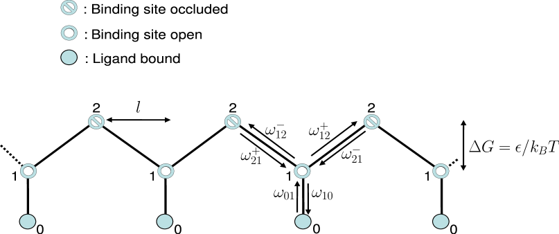
Figure 1: Schematic view of the three-state model for sliding of a nucleosome on a periodic DNA sequence of height $\Delta G=\epsilon k_{B}T$ and period $2l$. States 0, 1, and 2 denote states where the ligand is bound, unbound with its binding site open and unbound with its binding site closed, respectively. $\omega_{ij}^{+(-)}$ denote the rates of going from state $i$ to state $j$ to the right (left).

The presence of ligands affects the interaction of the nucleosome with the DNA, and we describe this as an additional state $0$ that branches off the state $1$ or $2$. When the ligand binds to the DNA, we assume that no sliding can happen, as confirmed by experiments Gottesfeld-02 . So the nucleosome waits until the ligand detaches from the DNA, and this will reduce the mobility of the nucleosome. The ligand may bind on the DNA either in state $1$ and $2$ depending on the location of its substrate that is a short DNA sequence. In this model we only consider the case where the ligand can bind to the DNA when the nucleosome is in state $1$. This is equivalent to $\Delta G>0$ in Fig. 1. In state 2 (5 bp, half the DNA pitch, away from state 1) the binding site is then inaccessible since it faces the octamer surface. Similar periodic sequential kinetic models with branching, jumping or deaths have been studied in Kolomeisky-00 . Especially in Ref. Farshid-04 the three state model in Fig. 1 has been examined in the same context as the current paper for special cases of the transition rates.

To model the dynamics of the histone, consider the one-dimensional lattice of Fig. 1. The nucleosome can hop to neighboring sites on this lattice with some specific rates. Assume that $l$ is the distance between sites $1$ and $2$ (which is half the period), and let $p_{i}(n,t)$ be the probability for the nucleosome to be in the states $i=0,1,2$, at position $x=nl$ and at time $t$. The $p_{i}(n,t)$ satisfy the master equation

$$\partial_{t}p_{0}(n,t) = \omega_{10}\,p_{1}(n,t)-\omega_{01}\,p_{0}(n,t)$$ (1)

$$\partial_{t}p_{1}(n,t) = \omega_{21}^{+}\,p_{2}(n-1,t)+\omega_{21}^{-}\,p_{2}(n+1,t)$$

$$+ \omega_{01}\,p_{0}(n,t)-(\omega_{12}^{+}+\omega_{12}^{-}+\omega_{10})\,p_{1}(n,t)$$

$$\partial_{t}p_{2}(n,t) = \omega_{12}^{+}\,p_{1}(n-1,t)+\omega_{12}^{-}\,p_{1}(n+1,t)$$ (3)

$$- (\omega_{21}^{+}+\omega_{21}^{-})\,p_{2}(n,t),$$

where $\omega_{ij}^{+}$ ($\omega_{ij}^{-}$) represents the rate of transition from state $i$ to neighboring state $j$ on the right (left); and $\omega_{10}$ ($\omega_{01}$) represents the binding (unbinding) rate of a ligand.

Let us introduce a vector $\vec{F}(\lambda,t)$, the components of which are generating functions of the position for each state $i$. These components are $F_{i}(\lambda,t)=\displaystyle\sum_{n}{e^{-\lambda nl}p_{i}(n,t)}$. The use of generating function reduces the space of configurations that is infinite, to only 3 states due to the periodicity of the system. It makes the calculations much more tractable. The master equation now becomes:

$$\partial_{t}\vec{F}(\lambda,t)=M(\lambda)\vec{F}(\lambda,t),$$ (4)

with

$$M(\lambda)=\left[\begin{array}[]{ccc}-\omega_{01}&\omega_{10}&0\\ &&\\ \omega_{01}&-\omega_{12}^{+}-\omega_{12}^{-}-\omega_{10}&\omega_{21}^{+}\,e^{-\lambda l}+\omega_{21}^{-}\,e^{\lambda l}\\ &&\\ 0&\omega_{12}^{+}\,e^{-\lambda l}+\omega_{12}^{-}\,e^{\lambda l}&-\omega_{21}^{+}-\omega_{21}^{-}\end{array}\right].$$ (5)

The solution of Eq. (4) is

$$\vec{F}(\lambda,t)=e^{M(\lambda)t}\vec{F}(\lambda,0).$$ (6)

After calculating the eigenvalues of the matrix $M$, one can see that at long time $t\rightarrow+\infty$ only the largest eigenvalue of $M$ that is denoted by $\sigma_{m}(\lambda)$, contributes to $\displaystyle\sum_{i}{F_{i}(\lambda,t)}=\left\langle e^{-\lambda nl}\right\rangle\sim e^{\sigma_{m}(\lambda)t}$. Note that the normalization condition for the probability implies that $\sigma_{m}(0)=0$. The eigenvalue $\sigma_{m}(\lambda)$ contains all the long time dynamical properties of the system, such as the velocity and the diffusion constant David-07 ; David-08 , since

$$\overline{v}=-\left.\frac{d\sigma_{m}}{d\lambda}\right|_{\lambda=0},$$ (7)

and

$$D=\left.\frac{1}{2}\frac{d^{2}\sigma_{m}}{d\lambda^{2}}\right|_{\lambda=0}.$$ (8)

One can expand $\sigma_{m}(\lambda)$ near $\lambda=0$ as $\sigma_{m}(\lambda)=-\overline{v}\lambda+D\lambda^{2}+O(\lambda^{2})$. Using this expansion in the eigenvalue equation, $\det\left[M-\sigma_{m}(\lambda)I_{3}\right]=0$, the velocity and the diffusion constant are derived as

$$\overline{v} = \frac{2\left(\omega_{12}^{+}\omega_{21}^{+}-\omega_{12}^{-}\omega_{21}^{-}\right)l}{S+\frac{\omega_{10}}{\omega_{01}}(\omega_{21}^{+}+\omega_{21}^{-})},$$ (9)

$$D = 2l^{2}\frac{\left(\omega_{12}^{+}\omega_{21}^{+}+\omega_{12}^{-}\omega_{21}^{-}\right)K+8\omega_{12}^{+}\omega_{12}^{-}\omega_{21}^{+}\omega_{21}^{-}+\frac{\omega_{10}}{\omega_{01}}J}{\left[S+\frac{\omega_{10}}{\omega_{01}}(\omega_{21}^{+}+\omega_{21}^{-})\right]^{3}},$$

with

$$S = \omega_{12}^{+}+\omega_{12}^{-}+\omega_{21}^{+}+\omega_{21}^{-},$$ (11)

$$K = {\omega_{12}^{+}}^{2}+{\omega_{12}^{-}}^{2}+{\omega_{21}^{+}}^{2}+{\omega_{21}^{-}}^{2}$$ (12)

$$+ 2\left(\omega_{12}^{+}\omega_{12}^{-}+\omega_{12}^{+}\omega_{21}^{-}+\omega_{21}^{+}\omega_{21}^{-}+\omega_{21}^{+}\omega_{12}^{-}\right),$$

$$J = \left(\omega_{12}^{+}\omega_{21}^{+}+\omega_{12}^{-}\omega_{21}^{-}\right)\times$$ (13)

$$\left(\omega_{21}^{+}+\omega_{21}^{-}\right)\left[2S+\frac{\omega_{10}}{\omega_{01}}\left(\omega_{21}^{+}+\omega_{21}^{-}\right)\right]$$

$$-2\left(\omega_{12}^{+}\omega_{21}^{+}-\omega_{12}^{-}\omega_{21}^{-}\right)^{2}\left[1-\frac{\omega_{21}^{+}+\omega_{21}^{-}}{\omega_{01}}\right].$$

It is worth to mention that in the ligand-free case the rate of going from site 1 to 0 is zero, $\omega_{10}=0$, and the model becomes equivalent to the two-state model that has been discussed in David-07 ; David-08 .

2 Kinetic rates in the absence of force

We assume that the nucleosome sliding in the absence of any external force is a passive process, which implies that there is no preference between left and right direction. Thus $\omega_{12}^{+}=\omega_{12}^{-}=\omega_{12}$ and $\omega_{21}^{+}=\omega_{21}^{-}=\omega_{21}$. Let us introduce $\kappa$ as the ratio of rates

$$\kappa\equiv\frac{\omega_{12}}{\omega_{21}}=e^{-\epsilon},$$ (14)

where $\epsilon=\Delta G/k_{B}T$ is the energy difference between the two states $1$ and $2$, and the above equality expresses the detailed balance condition.

We consider the binding chemical reaction of the ligand: $L+S\rightleftharpoons LS$, where $S$ is the substrate, i.e. the nucleosomal DNA, $L$ is the ligand and $LS$ is the ligand-substrate complex. From kinetics theory of first order chemical reactions, one can write $\omega_{10}=k_{+}[L][S]$ and $\omega_{01}=k_{-}[LS]$, such that the equilibrium constant of the chemical reaction is $K_{eq}=k_{+}/k_{-}=[LS]_{eq}/\left([L]_{eq}[S]_{eq}\right)$, in terms of equilibrium concentration of ligand $[L]_{eq}$, substrate $[S]_{eq}$ and complex $[LS]_{eq}$. Therefore the ratio

$$\eta\equiv\frac{\omega_{10}}{\omega_{01}}=K_{eq}\frac{[L][S]}{[LS]}=\frac{[LS]_{eq}}{[L]_{eq}[S]_{eq}}\frac{[L][S]}{[LS]},$$ (15)

quantifies the deviation away from equilibrium. In general, the substrate is in excess so that $[S]$ and $[S]_{eq}$ are both large, and also $[S]\simeq[S]_{eq}$. Furthermore, if one assumes that $[LS]\simeq[LS]_{eq}$, then $\eta\simeq[L]/[L]_{eq}$.

From Eq. (9), one finds that $\overline{v}=0$ as expected and the diffusion constant is:

$$D=\frac{2\;\omega_{12}\;l^{2}}{1+\eta+\kappa},$$ (16)

where $\omega_{12}$ can be calculated by Kramers rate theory in the limit $\epsilon\gg 1$.

The sequence dependent potential can be modelled as a periodic function $\beta U(x)=\frac{\epsilon}{2}\,\cos\left(\frac{\pi x}{l}\right)$ with $\beta=1/k_{B}T$ Kulic-03 . The time needed for the nucleosome to go from one minimum of this potential to the neighboring maximum, $\tau$, can be determined using the Kramers rate theory :

$$\frac{1}{\tau}=\frac{D_{0}}{2\pi k_{B}T}\sqrt{\left|U^{\prime\prime}(1)U^{\prime\prime}(2)\right|}\;e^{-\epsilon}=\frac{\pi\left|\epsilon\right|}{4l^{2}}D_{0}\;e^{-\epsilon},$$ (17)

where $D_{0}$ is the diffusion constant of the nucleosome without any potential barrier or ligand, $1$ and $2$ refer to the minimum and the maximum of the potential $U(x)$. From this we find $\omega_{12}$ for such a strong positioning sequence:

$$\omega_{12}=\frac{1}{2\tau}=\frac{\pi\epsilon}{8l^{2}}D_{0}\;e^{-\epsilon}\qquad{\rm for\;\;}\epsilon>0,$$ (18)

with the factor $\frac{1}{2}$ being the probability to go through the barrier $2$ from either direction Hanngi-1990 . It is worth to mention that in the limit $\epsilon\gg 1$ with ($\epsilon>0$, $\eta\geq 0$) when there is a sequence dependent potential for the nucleosome, one can find that:

$$D=\frac{\pi\epsilon\,e^{-\epsilon}}{4(1+\eta)}D_{0}.$$ (19)

In the case of random sequence of DNA, i.e in the absence of a sequence dependent potential, $\epsilon=0$ and then $\omega_{12}$ is simply equal to

$$\omega_{12}=\frac{D_{0}}{l^{2}},$$ (20)

and the diffusion constant can be found as

$$D=\frac{2D_{0}}{2+\eta}.$$ (21)

Putting in numbers, using realistic parameter values Kulic-03 $D_{0}\simeq 600\,bp^{2}/s$, $\epsilon=9$, $l=5\,bp$, $\eta=0$ in the absence of ligand, and $\eta\simeq 100$ in the presence of ligands our model predicts the time needed for a nucleosome to diffuse on a $70$ bp DNA, to be $78$ minutes without ligands and $131$ hours with the ligands which is consistent with the experimental observations Gottesfeld-02 . For a random sequence ($\epsilon=0$), in the presence ($\eta\simeq 100$) and the absence of ligands ($\eta\simeq 0$), the characteristic time for 70 bp diffusion are 3.5 min and 4 sec, respectively.

In the absence of ligands and for arbitrary sign of $\epsilon$, Eq. (19) becomes

$$D=\frac{\pi|\epsilon|\,e^{-|\epsilon|}}{4}D_{0}.$$ (22)

The above expression that has been derived with a discrete stochastic model, can be also derived using a continuous description in the limit $\epsilon\gg 1$. This can be done by considering a particle diffusing in the periodic potential $U(x)$, for which the diffusion coefficient is Hanngi-1990

$$D=D_{0}\langle e^{\beta U(x)}\rangle^{-1}\langle e^{-\beta U(x)}\rangle^{-1}.$$ (23)

Indeed $\langle e^{\beta U(x)}\rangle$ is a Bessel function, the asymptotic form of which is $2e^{\epsilon/2}/\sqrt{\pi\epsilon}$ for $\epsilon\gg 1$. From this Eq. (22) is recovered using Eq. (23).

2.1 Transcription-induced sliding

Up to now we considered thermally induced, undirected nucleosome sliding. Here we discuss the case when a force is applied to the nucleosome. As discussed in the introduction this situation might occur when an RNA polymerase encounters a nucleosome during transcription. A more microscopic model of such an encounter is presented in Ref. Laleh-08 . Note that we will assume that the polymerase does not unpeel the nucleosome, a case considered recently by T. Chou Chou-07 . Rapid progress in the field of micromanipulation experiments let us expect that there will be also soon data available where forces are directly applied to nucleosomes.

A force $F$ exerted on the nucleosome introduces a bias in the transition rates:

$$\omega_{12}^{+} = \omega\;e^{-\epsilon}\;e^{\theta_{1}^{+}f},$$ (24)

$$\omega_{21}^{-} = \omega\;e^{-\theta_{2}^{-}f},$$ (25)

$$\omega_{12}^{-} = \omega\;e^{-\epsilon}\;e^{-\theta_{1}^{-}f},$$ (26)

$$\omega_{21}^{+} = \omega\;e^{\theta_{2}^{+}f},$$ (27)

where $\theta_{i}^{\pm}$ are the load distribution factors Kolomeisky-00 , and $f\equiv Fl/k_{B}T$. Using detailed balance condition, one has $\theta_{1}^{+}+\theta_{1}^{-}+\theta_{2}^{+}+\theta_{2}^{-}=2$.

Putting these rates in Eq. (9), the velocity of the nucleosome can be found as

$$v=2\omega l\;e^{-\epsilon}\frac{e^{(\theta_{1}^{+}+\theta_{2}^{+})f}-e^{-(\theta_{1}^{-}+\theta_{2}^{-})f}}{e^{-\epsilon}\left(e^{\theta_{1}^{+}f}+e^{-\theta_{1}^{-}f}\right)+(1+\eta)\left(e^{\theta_{2}^{+}f}+e^{-\theta_{2}^{-}f}\right)}$$ (28)

The mobility of nucleosome is defined as

$$\mu\equiv\frac{1}{k_{B}T}\left.\frac{dv}{df}\right|_{f=0},$$ (29)

which gives

$$\mu=\frac{1}{k_{B}T}\frac{2\omega\kappa}{1+\eta+\kappa}l^{2}$$ (30)

Comparing this expression with Eq. (16) one finds the Einstein relation $\mu=D/(k_{B}T)$ verified.

3 Results

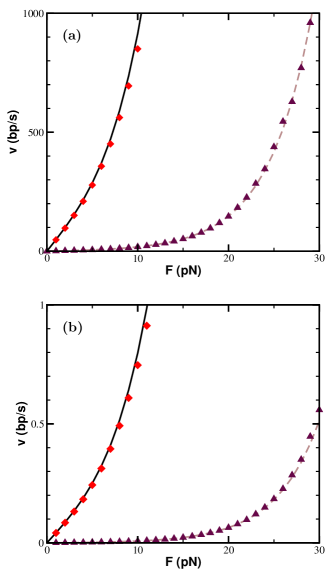
Figure 2: The velocity of the nucleosome versus the external force exerted on the DNA for (a) a random sequence of DNA ($\epsilon=0$) and (b) a positioning sequence with $\epsilon=9$ in two cases: the diamonds are simulation data for $\eta=0$ while the black solid line is plotted using theory, Eq. (28), the triangles are simulation data for $\eta=100$ while the brown dashed line is plotted using theory, again Eq. (28).

There are three physical quantities that affect the behavior of the system: the external force $F$, the sequence dependent part of the potential measured by $\epsilon$ and the ligand concentration $[L]$ that enters into $\eta$ through $\eta\simeq[L]/[L]_{eq}$. The physical behavior of the system is characterized by the velocity of the nucleosome repositioning along the DNA and its diffusive behavior. In this section, the results of the analytical approach described in the previous sections and of a computer simulation that is discussed in Appendix A, are presented.

We first consider the effect of an external force on the velocity of the nucleosome repositioning along the DNA. In Fig. 2 we plot the nucleosome velocity $v$ versus the applied force $F$ for the two limiting cases $\eta=0$ and $\eta=100$ of the experiments Gottesfeld-02 , on both random DNA and on a positioning sequence. As expected, the velocity of the nucleosome increases with the external force and there is a good agreement between the simulation results and the analytical approach. At zero force, the nucleosome shows purely diffusive behavior and there is no net velocity, cf. Fig. 2 at $F=0$. As soon as a force is applied, there is a bias in the transition rates and the nucleosome attains a drift velocity in the direction of the applied force. A positioning sequence of DNA leads to an effective potential barrier on the corkscrew path of the nucleosome Kulic-03 leading to a drift that is significantly smaller than on random DNA. The aforementioned behaviors are seen in Fig. 2.

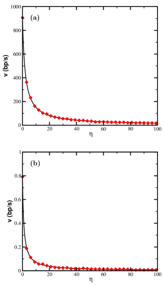
Figure 3: Velocity $v$ of the nucleosome versus $\eta$ in the presence of an external force $F=10\,pN$ on (a) a random basepair sequence ($\epsilon=0$) and (b) a positioning element ($\epsilon=9$). The red diamonds are the simulation results while the line is plotted using the analytical approach, Eq. 28.

Next we study how the ligands influence the sliding velocity. In Fig. 2 we see that for a given finite force the nucleosome velocity for the case $\eta=100$ is much smaller than in the absence of ligands, $\eta=0$. The effect of the ligand concentration on the drift velocity of the nucleosome for a typical external force, $F=10\,pN$, is shown in Fig. 3. As expected ligands block corkscrew sliding, lowering the overall drift velocity. For typical experimental numbers Gottesfeld-02 already a small concentration of ligands significantly lowers the drift, cf. Fig. 3.

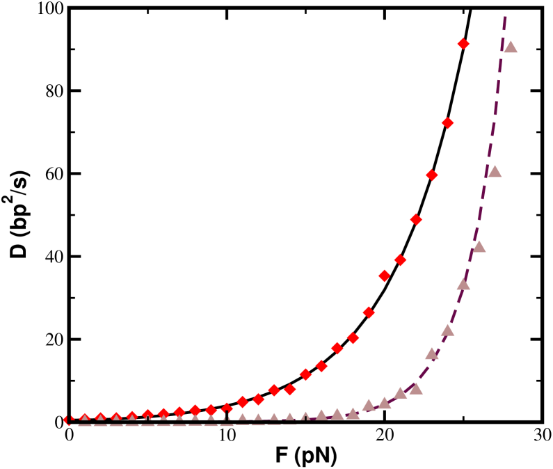
Figure 4: Diffusion constant $D$ of the nucleosome versus external force $F$ on a positioning sequence ($\epsilon=9$). The solid black line (red diamonds) and the brown dashed line (light brown triangles) are the theoretical (simulation) results for $\eta=0$ and $\eta=100$.

Another parameter that provides information about the system is the diffusion constant of the nucleosome, $D$. The behavior of $D$ versus both the external force and the ligand concentration has been checked on for random DNA and a positioning sequence. In Fig. 4 it can be seen that $D$ increases with $F$. Using a simple two state model can help us to understand the behavior of the diffusion constant in terms of force $F$. This simple model has been explained in Appendix B. We see that in the presence of external force, the diffusion constant of the particle becomes larger when the force is increased.

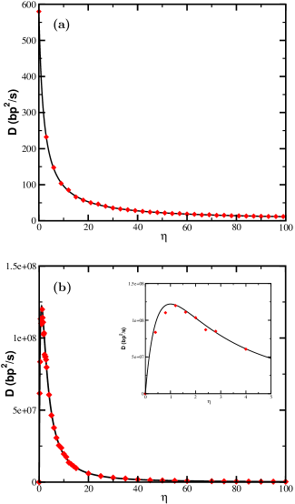
Figure 5: Nucleosome diffusion constant $D$ versus $\eta$ for random DNA ($\epsilon=0$) for two different forces: (a) $F=0\,pN$ and (b) $F=10\,pN$ (the inset gives a zoomed view showing the non-monotonous behavior for small $\eta$-values). The red diamonds are the simulation results while the lines use the analytical approach, Eq. LABEL:explicit_D.

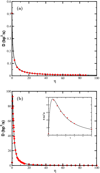
Figure 6: The diffusion constant of the nucleosome versus $\eta$ in the case of a positioning sequence with $\epsilon=9$ for two different forces: (a) $F=0\,pN$ and (b) $F=10\,pN$. The inset is the zoomed-in plot showing the behavior of the diffusion constant for small values of $\eta$. The red diamonds are the simulation results while the lines are plotted using the analytical approach.

We present the behavior of the diffusion constant versus $\eta$, for two different forces, $F=0pN$ and $F=10\,pN$, in Figs. 5 and 6. Naively one would expect that at a fixed external force the diffusion constant decreases with $\eta$ since an increase of the ligand concentration leads to a higher probability to have a ligand bound that then suppresses diffusion. For zero force the diffusion constant does indeed follow this expectation, cf. Figs. 5(a) and 6(a). Interestingly, in the presence of a nonzero external force the behavior of the diffusion constant versus $\eta$ differs dramatically from this expectation. For $\eta\lesssim 1$, $D$ increases with $\eta$, and then decreases as $\eta$ goes to infinity (Figs. 5(b) and 6(b)). For random (positioning) DNA the maximal value of the diffusion constant is five (two) orders of magnitude larger than the value in the absence of ligands.

For $\eta\ll 1$ the diffusion constant in 3-state model behaves as the 2-state model with a correction like $D_{\rm{3-state}}=D_{\rm{2-state}}+O(\eta)$. For large values of $\eta$, as can be seen in Eq. (LABEL:explicit_D), the diffusion constant changes as $D\propto 1/\eta$ and the diffusion constant decreases as $\eta$ increases. The $\eta$ at which $D$ attains its maximum $\eta^{*}$ can be calculated from Eq. (LABEL:explicit_D) and is shown in Fig. 7 as a function of $F$ for two cases of random and positioning DNA. As can be seen in this figure, at not very small forces, $\eta^{*}$ is equal to $1$ for random DNA and $0.5$ for the positioning sequence. Since at large forces the positive rates $\omega^{+}$ dominate, the diffusion constant, Eq. (LABEL:explicit_D), simplifies to

$$D=2l^{2}\frac{\eta(\omega_{12}^{+}\omega_{21}^{+})^{2}\omega_{21}^{+}}{\omega_{01}\left[\omega_{21}^{+}(\eta+1)+\omega_{12}^{+}\right]^{3}}.$$ (31)

Setting the derivative of $D$ with respect to $\eta$ equal to zero, one obtains

$$\eta^{*} = \frac{\omega_{12}^{+}+\omega_{21}^{+}}{2\omega_{21}^{+}}$$ (32)

$$= \frac{1+e^{-\epsilon+(\theta_{1}^{+}-\theta_{2}^{+})f}}{2},$$

where we have used Eqs. (24)–(27). For the case $\theta_{i}^{\pm}=1/2$ the force dependent term drops out and we find $\eta^{*}=(1+e^{-\epsilon})/2$ and especially $\eta^{*}=1$ for random DNA. We shall come back to this point in the discussion section. In Fig. 7, the behavior of $\eta^{*}$ is plotted versus the external force in the case of $\theta_{i}^{\pm}=1/2$.

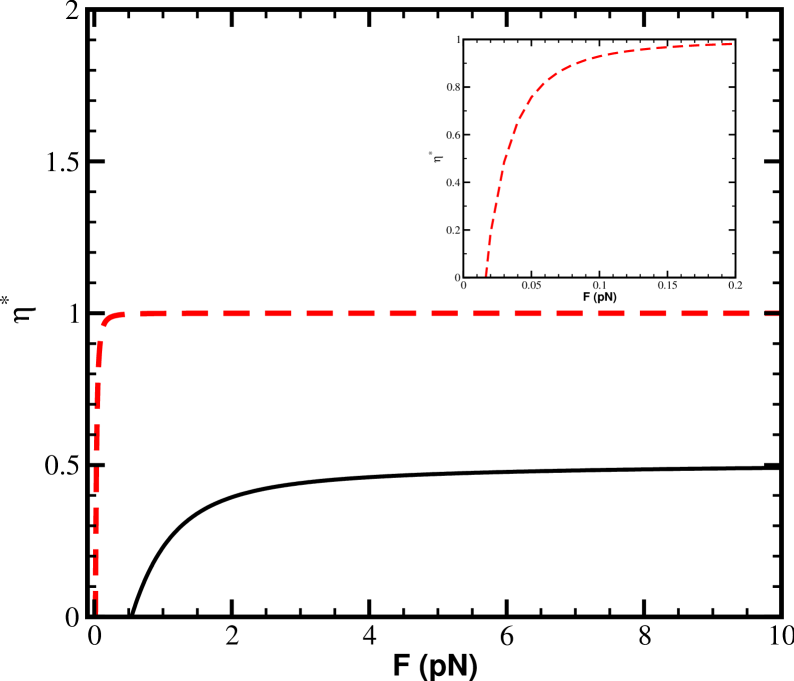
Figure 7: $\eta^{*}$ versus $F$ for the case $\theta_{i}^{\pm}=1/2$ for random DNA (dashed line) and a nucleosome positioning element (solid line). The lines are drawn using Eq. 32.

Let us now discuss the behavior of the diffusion constant versus $\eta$ for small values of $\eta$, i.e. for $\eta\ll 1$. Through an expansion of the exact expression we obtain

$$D=A_{0}(f)+A_{1}(f)\eta+O(\eta^{2}),$$ (33)

where $A_{0}$ and $A_{1}$ are functions of $f$ that are given in Appendix C. It is convenient to expand $A_{1}(f)$ as a function of $f$:

$$A_{1}(f)=\left.\frac{\partial D}{\partial\eta}\right|_{\eta=0}=\alpha(\beta_{0}+\beta_{1}f^{2})+O(f^{4}),$$ (34)

where $\alpha$, $\beta_{0}$, and $\beta_{1}$ are functions defined in Appendix C. Since $\alpha>0$ and $\beta_{0}<0$, we have $\partial D/\partial\eta<0$ for both random and positioning sequence of DNA at $f=0$ that can indeed be seen in the plots of diffusion constant $D$ versus $\eta$ shown in Figs. 5(a) and 6(a). When $\beta_{1}$ becomes positive, there is a threshold in force that is $f_{T}=\sqrt{-\beta_{0}/\beta_{1}}$ such that for $f>f_{T}$ the derivative of $D$ with respect to $\eta$ is positive for small $\eta$-values. From the expression of the coefficients derived in Appendix C, the value of $f_{T}$ is the following function of $\epsilon,\omega$ and $\omega_{01}$:

$$f_{T}=\frac{\sqrt{2}\left(1+e^{-\epsilon}\right)}{\left[-3+e^{-\epsilon}\left(5-6e^{-\epsilon}\right)+4e^{-\epsilon}\left(1+e^{-\epsilon}\right)\frac{\omega}{\omega_{01}}\right]^{1/2}}.$$ (35)

Putting in numbers, $\omega_{01}=0.001\;s^{-1}$ and $\omega=D_{0}/l^{2}\simeq 24\;s^{-1}$, we find $f_{T}\simeq 0.48$ that is equivalent to $F\simeq 0.016\;pN$ for a random sequence of DNA. In the case of positioning sequence of DNA the rate of $\omega$ changes to $\omega=\pi\epsilon D_{0}/(8l^{2})\simeq 85\;s^{-1}$ and we find $f_{T}\simeq 0.23$ that is equivalent to $F\simeq 0.55\;pN$. In Fig. 7 the behavior of $\eta^{*}$ as a function of $F$ is shown for both random and positioning sequence of DNA. We note that the force value for which $\eta^{*}=0$ corresponds to the threshold force given by Eq. (35).

How can the surprising non-monotonous behavior of $D$ as a function of $\eta$ of a nucleosome driven by the application of a force be explained, especially the strongly enhanced fluctuations around $\eta^{*}$ with $D(\eta^{*})\gg D(\eta=0)$? Obviously the fluctuations of position of this driven nucleosome in the presence of ligands are of different origin than the ones in the absence of ligands. For sufficiently large forces the nucleosome mostly steps in the direction of the force or – if the nucleosome is in state 1 – a ligand might bind. The latter event stops the drifting nucleosome for a while and is thus a source of fluctuations of completely different origin, because this introduces some waiting time before hopping from states 1. The higher the concentration of ligands, i.e. the higher the value of $\eta$, the more often these events occurs, increasing their contribution to the overall fluctuation of the nucleosome, which are measured by the diffusion coefficient. This is the case up to a critical value of $\eta$, named $\eta^{*}$, which is force dependent. Further addition of ligands populates the state 0 so much that the nucleosomes gets frequently stuck, decreasing its diffusion constant.

4 Discussion

In our model the external force changes the local rates from sites $1$ to $2$ and vise versa. This is because the force produces internal stress on the nucleosomal DNA that introduces a bias in the dynamics. This assumption can be verified by considering the microscopic details of the interaction of the nucleosome with the DNA that will be presented in a forthcoming publication Laleh-08 .

In the above treatment we assumed that both binding and unbinding rates of ligands to the DNA do not depend on the external force. The typical length of a ligand site is about 6-7 bps and the DNA length between two adjacent binding sites is 10 bps. Even at the highest forces considered here (30 pN) the probability of having a defect in a ligand binding region is close to zero Laleh-08 so that we expect that its influence on the ligand rates can be neglected.

It is also important to point out that the load distribution factors $\theta_{i}^{\pm}$ have an effect on the diffusion constant. We assumed that all $\theta_{i}^{\pm}$ are equal to $\frac{1}{2}$. By changing the values of $\theta_{i}^{\pm}$ the overall behavior of all plots does not change, although the precise values of the diffusion coefficient and even the curvature of the plots can be affected. For instance, the value of $\eta^{*}$ at which $D$ is maximized depends on the values of $\theta_{i}^{\pm}$ as can be seen from Eq. (32). The microscopic details of the interaction between the DNA and the nucleosome determine the values of the distribution factors. For a random sequence there is no reason to have different rates for backward and forward steps of the nucleosome along the DNA. Therefore, one finds that for large values of the external force, $\eta^{*}$ converges to $1$. For a DNA positioning sequence, the values of $\theta_{i}^{\pm}$ could in principle depend on the sequence. The exact value of these coefficients can only be determined from experimental data or from a more detailed modelling of the transition state. We have arbitrarily chosen them to be $1/2$ for the plots. Note that if $\theta_{1}^{+}<\theta_{2}^{+}$ then $\eta^{*}|_{F\rightarrow\infty}=0.5$, the same value as in our case $\theta_{1}^{+}=\theta_{2}^{+}$, while for $\theta_{1}^{+}>\theta_{2}^{+}$, $\eta^{*}$ increases as $F$ is increased and one has $\eta^{*}|_{F\rightarrow\infty}\rightarrow\infty$.

5 Acknowledgments

We are thankful to K. Mallick and H. Fazli for valuable discussions. D. L. acknowledges support from the the Indo-French Center CEFIPRA (grant 3504-2) and F. M. acknowledges support from CNRS and the hospitality of Laboratoire de Physico-Chimie Théorique, UMR 7083, ESPCI in Paris where this work was initiated.

6 Appendix

Appendix A The algorithm of the simulation

The 3-state model presented in this paper is simulated using a “Random Selection Method” random alg . It is defined in terms of the transition rates $\omega_{ij}^{\pm}$ that give the probabilities per unit time for going from state $i$ to state $j$ in the plus/minus direction. If the system is at time $t$ in the state $i$, a transition to the neighboring state $j$ happens at time $t\,+\,\Delta t$ with the finite probability $P_{ij}^{\pm}=\Delta t\,\omega_{ij}^{\pm}$.

For each step, a random number $0\leq\xi<1$ is drawn. Depending on its value and the state of the system a decision is taken:

$$\rm{state}:0 \rightarrow 1~{}\quad~{}\rm{if}~{}0\leq\xi<P_{01},$$

$$\rm{state}:0 \rightarrow 0~{}\quad~{}\rm{otherwise}$$

$$\rm{state}:1 \rightarrow 0~{}\quad~{}~{}\rm{if}~{}0\leq\xi<P_{10},$$

$$\rm{state}:1 \rightarrow 2^{+}~{}\quad\rm{if}~{}P_{10}\leq\xi<P_{10}+P^{+}_{12},$$

$$\rm{state}:1 \rightarrow 2^{-}~{}\quad\rm{if}~{}P_{10}+P_{12}^{+}\leq\xi<P_{10}+P_{12}^{+}+P_{12}^{-},$$

$$\rm{state}:1 \rightarrow 1~{}\quad~{}~{}\rm{otherwise}$$

$$\rm{state}:2 \rightarrow 1^{+}~{}\quad\rm{if}~{}0\leq\xi<P_{21}^{+},$$

$$\rm{state}:2 \rightarrow 1^{-}~{}\quad\rm{if}~{}P_{21}^{+}\leq\xi<P_{21}^{+}+P_{21}^{-},$$

$$\rm{state}:2 \rightarrow 2~{}\quad~{}~{}\rm{otherwise}.$$

For the next time step, from $t+\Delta t$ to $t+2\Delta t$, the procedure is repeated again. The time step $\Delta t$ is chosen small enough, such that for each step the condition $\sum\omega_{ij}^{\pm}\Delta t<1$ is satisfied, where the sum is taken over the probabilities of all possible transitions from state $i$.

This algorithm is similar to the one of Gillespie Gillespie-77 , except for the fact that we use here a constant time step whereas for the Gillespie algorithm the time step is a random variable. Both algorithms converge to the same steady state albeit after different times as we also checked for our model. The steady state probabilities for the three states are obtained by setting the time derivatives of the probabilities in Eqs. (1)–(3) to zero:

$$p_{0} = \frac{\eta}{1+\eta+e^{-\epsilon}},$$ (36)

$$p_{1} = \frac{1}{1+\eta+e^{-\epsilon}},$$ (37)

$$p_{2} = \frac{e^{-\epsilon}}{1+\eta+e^{-\epsilon}},$$ (38)

a result that has been previously obtained in Ref. Farshid-04 . We let the simulation run for a long time (from $t_{0}$ to $t_{N}$ with $t_{i}=i\Delta t$, $N\gg 1$) to be sure that the system has reached equilibrium. Then averaged over $M$ ensembles with $M\gg 1$, the mean velocity and the diffusion constant is determined by

$$v=\frac{\sum_{r=1}^{M}(X_{r}(t_{N})-X_{r}(t_{1}))}{N\Delta t\times M},$$ (39)

and $D$ is determined as the slope of the plot of $\sum_{r=1}^{M}X_{r}^{2}/M-(\sum_{r=1}^{M}X_{r}/M)^{2}$ versus $2\sum_{r=1}^{M}t_{r}/M$.

The time steps used for the simulation are less than $0.001$, depending on the simulated case. The time goes to $10^{5}\,s$, and the number of ensembles are $M=2000$. The used parameters for the simulation are $\theta_{i}^{\pm}=1/2,~{}i=1,2$ and $\omega$ is determined from to Eq. (18) and Eq. (20) for the positioning and random DNA sequence respectively. Also using the experimental data, the typical time needed for a ligand to unbound from the DNA is some minutes and $\omega_{01}=0.001\,s^{-1}$.

Appendix B The behavior of the diffusion constant versus the external force in a simple two state model

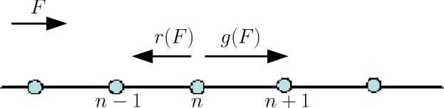
Figure 8: The two state problem used to explain the behavior of the diffusion constant versus the applied force. The external force, $F$, changes the jumping rates of the particle, which are shown by $g(F)$ and $r(F)$.

To check the effect of force on the diffusion constant, let us assume a simple two state model in which the external force changes the rates as shown in Fig. 8. The position of the particle in the mentioned lattice model is denoted by $n$. By definition, the diffusion constant is written as

$$D\equiv\frac{1}{2}\lim_{t\rightarrow\infty}\frac{\partial}{\partial t}\left[\langle n^{2}\rangle-\langle n\rangle^{2}\right],$$ (40)

where $\langle A\rangle$ denotes the average of quantity $A$ that is given by $\langle A\rangle=\sum_{n}A_{n}P_{n}$. $P_{n}$ is the probability for the particle to be in the position $n$.

The master equation governing this system can be written as

$$\frac{d\,P_{n}}{dt}=r(F)P_{n+1}+g(F)P_{n-1}-\left[r(F)+g(F)\right]P_{n},$$ (41)

where the force is denoted by $F$, $a$ is the jump length, and $g(F)$ and $r(F)$ are the force-dependent rates for going to the right and left, respectively. Depending on the direction the force is exerted on the system, one of these rates increases and one decreases. Here, we have assumed that the force pushes the system to the right, so $g(F)$ increases with $F$ while $r(F)$ decreases with $F$. Then a simple calculation leads to:

$$\frac{\partial}{\partial t}\langle n^{2}\rangle = 2\left[g(F)-r(F)\right]\langle n\rangle+g(F)+r(F),$$ (42)

$$\frac{\partial}{\partial t}\langle n\rangle^{2} = 2\left[g(F)-r(F)\right]\langle n\rangle,$$ (43)

where we have used:

$$\frac{\partial}{\partial t}\langle A\rangle = \sum_{n}A_{n}\frac{\partial}{\partial t}P_{n},$$ (44)

$$\frac{\partial}{\partial t}\langle A\rangle^{2} = 2\langle A\rangle\frac{\partial}{\partial t}\langle A_{n}\rangle,$$ (45)

and

$$\sum_{n}P_{n}=1.$$ (46)

Using Eqs. (42) and (43), one finds the diffusion constant as following:

$$D=\frac{g(F)+r(F)}{2}.$$ (47)

If the rates in the absence of the external force are denoted by $\omega$, the external force, $F$, changes the jumping rates of the particle to $g(F)=\omega\exp\left[{+Fa/(2k_{B}T)}\right]$ and $r(F)=\omega\exp\left[{-Fa/(2k_{B}T)}\right]$. Using Eq. (47) and the mentioned rates in the presence of external force, the diffusion constant is found as

$$D=\frac{\omega}{2}\left(e^{+Fa/2k_{B}T}+e^{-Fa/2k_{B}T}\right).$$ (48)

This explains the behavior of our results for the diffusion constant mentioned in the text.

Appendix C The explicit forms of the auxiliary functions

In this appendix we give the explicit form of the constants used in the Eqs. (33) and (34). First we expand $D$ for $\eta\rightarrow 0$:

$$D = \frac{B_{0}+B_{1}\eta+B_{3}\eta^{2}}{[S+B_{2}\eta]^{3}}$$ (49)

$$= \frac{B_{0}}{S^{3}}+\frac{B_{1}S-3B_{0}B_{2}}{S^{4}}\eta+O(\eta^{2}),$$

where

$$B_{0} = 2l^{2}\left[K(\omega_{12}^{+}\omega_{21}^{+}+\omega_{12}^{-}\omega_{21}^{-})+8\omega_{12}^{+}\omega_{21}^{+}\omega_{12}^{-}\omega_{21}^{-}\right],$$

$$B_{1} = 2l^{2}[2(\omega_{12}^{+}\omega_{21}^{+}+\omega_{12}^{-}\omega_{21}^{-})(\omega_{21}^{+}+\omega_{21}^{-})S$$

$$-2(\omega_{12}^{+}\omega_{21}^{+}-\omega_{12}^{-}\omega_{21}^{-})^{2}(1-\frac{\omega_{21}^{-}+\omega_{21}^{+}}{\omega_{01}})],$$

$$B_{2} = \omega_{21}^{+}+\omega_{21}^{-},$$

$$B_{3} = 2l^{2}\left[(\omega_{21}^{-}+\omega_{21}^{-})^{2}(\omega_{12}^{+}\omega_{21}^{+}+\omega_{12}^{-}\omega_{21}^{-})\right].$$

From this follow the expansion coefficients in Eq. (33):

$$A_{0}(f) = \frac{B_{0}}{S^{3}},$$ (50)

$$A_{1}(f) = \frac{B_{1}S-3B_{0}B_{2}}{S^{4}}.$$ (51)

Finally we provide here the behavior of $A_{1}(f)$ for small forces. Using Eqs. (24)–(27) with $\theta_{i}^{\pm}=0.5$, the expansion of $B_{i}(f)$ for small forces can be written as

$$S = 2\omega(e^{-\epsilon}+1)(1+\frac{f^{2}}{4}),$$

$$B_{0} = 8\omega^{4}e^{-\epsilon}(e^{-\epsilon}+1)^{2}$$

$$+ 4\omega^{4}e^{-\epsilon}\left[2+2e^{-2\epsilon}+(e^{-\epsilon}+1)^{2}\right]f^{2},$$

$$\frac{B_{1}}{2l^{2}} = 16\omega^{4}e^{-\epsilon}(e^{-\epsilon}+1)$$

$$+ \left[16\omega^{4}e^{-2\epsilon}\left(1+\frac{\omega}{\omega_{01}}+24\right)\right]f^{2},$$

$$\frac{B_{2}}{2l^{2}} = 2\omega(1+\frac{f^{2}}{4}).$$

Consequently,

$$A_{1}(f) = \frac{16l^{2}\omega^{5}}{S^{4}}e^{-\epsilon}\left\{-2\left(1+e^{-\epsilon}\right)^{2}\right.$$

$$+ \left.\left[-3+e^{-\epsilon}\left(5-6e^{-\epsilon}\right)+4e^{-\epsilon}\left(1+e^{-\epsilon}\right)\frac{\omega}{\omega_{01}}\right]\right\},$$

Using these expansions and Eq. (34), one can write:

$$\alpha = \frac{16l^{2}\omega^{5}}{S^{4}}e^{-\epsilon},$$ (53)

$$\beta_{0} = -2(1+e^{-\epsilon})^{2},$$ (54)

$$\beta_{1} = -3+e^{-\epsilon}\left(5-6e^{-\epsilon}\right)+4e^{-\epsilon}\left(1+e^{-\epsilon}\right)\frac{\omega}{\omega_{01}}.$$ (55)

References

- (1) K. Luger, A. W. Mäder, R. K. Richmond, D. F. Sargent, and T. J. Richmond, Nature 389, 251 (1997).
- (2) J. Widom, Proc. Natl. Acad. Sci. USA 89, 1095 (1992).
- (3) K. J. Polach and J. Widom, J. Mol. Biol. 254, 130 (1995).
- (4) G. Li, M. Levitus, C. Bustamante, and J. Widom, Nature Struct. Mol. Biol. 12, 46 (2005).
- (5) W. Möbius, R. A. Neher, and U. Gerland, Phys. Rev. Lett. 97, 208102 (2006).
- (6) P. Beard, Cell 15, 955 (1978).
- (7) S. Pennings, G. Meersseman, and E. M. Bradbury, J. Mol. Biol. 220, 101 (1991). G. Meersseman, S. Pennings, and E. M. Bradbury, EMBO J. 11, 2951 (1992).
- (8) A. Flaus and T. J. Richmond, J. Mol. Biol. 275, 427 (1998).
- (9) A. Flaus and T. Owen-Hughes, Biopolymers 68, 563 (2003).
- (10) H. Schiessel, J. Phys.: Condens. Matter 15, R699 (2003).
- (11) P. Ranjith, J. Yan, and J. F. Marko, Proc. Natl. Acad. Sci. USA 104, 13649 (2007).
- (12) H. Schiessel, J. Widom, R. F. Bruinsma, and W. M. Gelbart, Phys. Rev. Lett. 86, 4414 (2001).
- (13) I. M. Kulić and H. Schiessel, Biophys. J. 84, 3197 (2003).
- (14) I. M. Kulić and H. Schiessel, Phys. Rev. Lett. 91, 148103, (2003).
- (15) F. Mohammad-Rafiee, I. M. Kulić, and H. Schiessel, J. Mol. Biol. 344, 47 (2004).
- (16) E. Segal et al., Nature 442, 772 (2006).
- (17) J.M. Gottesfeld, J.M. Belitsky, C. Melander, P.B. Dervan, and K. Luger, J. Mol. Biol. 321, 249 (2002).
- (18) V. M. Studitsky, D. J. Clark, and G. Felsenfeld, Cell 76, 371 (1994).
- (19) J. Bednar, V. M. Studitsky, S. A. Gregoryev, G. Felsenfeld, and C. L. Woodcock, Mol. Cell 4, 377 (1999).
- (20) B. ten Heggeler-Bodier, C. Schild-Poulter, S. Chapel, and W. Wahli, EMBO J. 14, 2561 (1995); B. ten Heggeler-Boudier, S. Muller, M. Monestier and W. Wahli, J. Mol. Biol. 299, 853 (2000).
- (21) A.W.C. Lau, D. Lacoste, and K. Mallick, Phys. Rev. Lett. 99, 158102 (2007).
- (22) D. Lacoste, A.W.C. Lau, and K. Mallick, http://fr.arxiv.org/abs/0801.4152, in press to appear in Phys. Rev. E.
- (23) A. B. Kolomeisky and M. E. Fisher, Physica A 279, 1 (2000).
- (24) P. Hänggi, P. Talkner and M. Borkovec, Rev. Mod. Phys. 62, 251 (1990).
- (25) L. Mollazadeh-Beidokhti, F. Mohammad-Rafiee, and H. Schiessel, in preparation.
- (26) T. Chou, Phys. Rev. Lett. 99, 058105 (2007).
- (27) T. H. Cormen, C. E. Leiserson, R. L. Rivest, and C. Stein. Introduction to Algorithms, Second Edition. MIT Press and McGraw-Hill (1990).
- (28) D. T. Gillespie, J. Phys. Chem. 81, 2340 (1977).