Complementarity of Future Dark Energy Probes
Abstract
In recent years a plethora of future surveys have been suggested to constrain the nature of dark energy. In this paper we adapt a binning approach to the equation of state factor “w” and discuss how future weak lensing, galaxy cluster counts, Supernovae and baryon acoustic oscillation surveys constrain the equation of state at different redshifts. We analyse a few representative future surveys, namely DES, PS1, WFMOS, PS4, EUCLID, SNAP and SKA, and perform a principal component analysis for the “w” bins. We also employ a prior from Planck cosmic microwave background measurements on the remaining cosmological parameters. We study at which redshifts a particular survey constrains the equation of state best and how many principal components are significantly determined. We then point out which surveys would be sufficiently complementary. We find that weak lensing surveys, like EUCLID, would constrain the equation of state best and would be able to constrain of the order of three significant modes. Baryon acoustic oscillation surveys on the other hand provide a unique opportunity to probe the equation of state at relatively high redshifts.
keywords:
cosmology:observations – cosmology:theory – dark energy1 Introduction
One of the most challenging puzzles in modern physics is the cause for the observed accelerated expansion of the Universe. The renewed interest in accelerating cosmologies was born out of Type Ia Supernovae observations a decade ago (Perlmutter et al., 1997; Riess et al., 1998; Perlmutter et al., 1999). In the meantime the cosmic concordance model (Ostriker & Steinhardt, 1995) has been confirmed by complementary observations of the Cosmic Microwave Background (CMB) (Spergel et al., 2003), the large scale distribution of galaxies (Efstathiou et al., 2002; Tegmark et al., 2004) and clusters of galaxies (Allen et al., 2004; Rapetti et al., 2005). In addition observations of large scale CMB anisotropies (Scranton et al., 2003; Padmanabhan et al., 2005) and Baryon Acoustic Oscillations (BAO) in the matter distribution (Cole et al., 2005; Eisenstein et al., 2005) also indicate the presence of late time acceleration in the Universe.
The simplest way to model an accelerated expansion in the Universe is by including a cosmological constant in Einstein’s equations of gravity. However, the introduction of a cosmological constant requires an extreme fine tuning of the initial conditions of our Universe to about 120 orders of magnitude. This motivates the search for alternative explanations for the speeding up of the expansion rates, although there have been recent successes in obtaining universes with the observed cosmological constant in a range of the multi verses of the meta-stable vacua of the string theory landscape (Kachru et al., 2003). This, in connection with the anthropic principle (Weinberg, 1987; Efstathiou, 1995; Bousso, 2006; Peacock, 2007; Cline et al., 2007), could motivate the observed value of the cosmological constant. Nevertheless, it is still valid to seek other alternatives to a cosmological constant. One approach is to introduce a dynamical scalar field, usually dubbed Quintessence, which is either slowly rolling down a potential or is trapped in a false vacuum state (Wetterich, 1988; Peebles & Ratra, 1988; Ratra & Peebles, 1988; Frieman et al., 1995; Ferreira & Joyce, 1998; Zlatev et al., 1999; Albrecht & Skordis, 2000). These models can lead to cosmic acceleration with less fine tuning. Another possibility was that the Universe is permeated by a network of cosmic defects, which also acts like a source in the energy-momentum tensor and can lead to accelerated expansion (Battye et al., 1999; Battye & Moss, 2005). The dynamical evolution of the Universe in Quintessence or defect based models is governed by the equation of state of the dominant components. The equation of state is given by the ratio of the pressure to the density of these fluids. For a cosmological constant this is -1. However dynamical dark energy models can deviate from this value and the ratio can also vary with time. Typically the ratio is named “”. The precise measurement of the value of “” is hence one of the foremost tasks for observational cosmology. Any significant measurement of a deviation of “” from -1, would be a major result. Currently conservative constraints on “” are in the region of (Tegmark et al., 2004; Astier et al., 2006).
Up to now, it has been difficult to make any connection between suggested Quintessence fields and fundamental theories. Another possibility to obtain accelerated expansion is the modification of Einstein’s gravity on large scales. There are two approaches along these lines. One is to modify a proposal by Starobinskij (1980), which includes higher order curvature terms in the gravitational action to obtain accelerated expansion in the early Universe. This has been adapted to explain the observed accelerated expansion (Carroll et al., 2004; Carroll et al., 2005). Another approach is to obtain effective four dimensional Friedman equations, from a five or higher dimensional theory, where our standard model is confined to a brane, with only gravity allowed to leak out into the extra dimension(s) (Dvali et al., 2000; Deffayet et al., 2002; Dvali & Turner, 2003). Although these models might have structural problems such as ghosts (Koyama, 2005; De Felice et al., 2006) it is a worthwhile exercise to explore their cosmological phenomenology. In particular they are different to Quintessence models in the way structures grow in the Universe (Song, 2005; Koyama, 2006). Finally it is possible, at least in theory, that the observed acceleration is an effect, which results from an averaging procedure to describe the large scale dynamics of an intrinsically inhomogeneous Universe (Buchert, 2005).
All the models described above have in common that they can, but don’t have to, deviate from the evolution of a so called -cold dark matter (CDM) Universe consisting of a cosmological constant and dark matter. Effectively the background evolution for all these models can be mimicked by a suitable chosen additional component in the energy-momentum tensor. Hence the quest for “” goes beyond its usual application to Quintessence models, although they are the only models where there is actually a physical meaning associated with “”. It is therefore an interesting question to ask if “” is different from -1 the value for a cosmological constant. The first attempt to address this question is to look for different constant values of “”. However, this approach is very restrictive given that dark energy models allow for evolving equation of state factors “w” (Weller & Albrecht, 2001, 2002; Maor et al., 2002). Hence it is important to allow for a time varying equation of state parameter “”. A simple Taylor expansion in redshift (Weller & Albrecht, 2002) is too restrictive if we want to include data sets which are sensitive to high redshifts, like the CMB. A more successful approach is to parameterise a time varying equation of state with a Taylor expansion in the scale factor , like (Chevallier & Polarski, 2001; Linder, 2003). This was also the parameterisation of choice adapted by the Dark Energy Task Force (DETF) (Albrecht et al., 2006). The DETF chose this parameterisation to be able to compare different proposed surveys on an equal footing. In addition this parameterisation allows to some extend the distinction of two subclasses of Quintessence models, namely freezing and thawing out models (Linder, 2006).
In this paper we want to pursue a more general approach. In order to figure out the redshift sensitivity to the dark energy density, or better its time derivative, we will bin the equation of state in redshift (Huterer & Starkman, 2003; Crittenden & Pogosian, 2005; Huterer & Peiris, 2007; Albrecht & Bernstein, 2007; Sullivan et al., 2007). Although, there are some ambiguities how to exactly perform the binning (de Putter & Linder, 2007), the binning approach is in general the most model independent approach to fit for the background evolution of the Universe. Note that this approach is inherently related to the weighting function method (Deep Saini et al., 2003; Simpson & Bridle, 2006) in the limit of an infinite number of bins.
We are now faced with the difficult task of selecting surveys to pursue our analysis. We emphasize that our selection is subjective and our aim is that we have at least one representative survey for each of the probes we are discussing. In this introduction we will mention briefly the surveys and what their technical specification is expected to be, while we describe how they exploit particular cosmological probes in the sections where we discuss constraint from the different probes.
We start with Stage II surveys according to the classification by the DETF (Albrecht et al., 2006). Already online in its simplest configuration is the PANoramic Survey Telescope and Rapid Response System (PAN-Starrs)111see at: pan-starrs.ifa.hawaii.edu. PAN-Starrs in it’s full configuration will consist of four 1.8 metre telescopes, equipped with a wide field camera with a field of view of 7 arcminutes and a total of 1.4 Gigapixels. Currently only one of the four planned telescopes is deployed. We refer to this setup as PAN-Starrs1 (PS1) in contrast to the full setup PAN-Starrs4 (PS4). The PAN-Starrs survey is planned to take exposures of seconds in each of the grizy filters in the PS1 configuration and should go much deeper in the PS4 configurations with grizy filters. One of the surveys with PS1 will be a nearly all sky, , survey up to a median redshift of . The nearly all sky survey is hoped to be exploited for large scale structure and BAOs (Peebles & Yu, 1970; Hu & Eisenstein, 1998; Blake & Glazebrook, 2003) experiments as well as weak gravitational lensing observations. The medium deep survey will be suitable for cosmological constraints with Type Ia SNe out to redshifts of . PS1 in the DETF category is a Stage II survey, while PS4 is Stage III.
Another survey already deployed, which is relevant to dark energy science, is the South Pole Telescope (SPT) (Ruhl et al., 2004). The SPT is a 10 metre telescope with a bolometer array in its focal plane, designed to detect thousands of clusters of galaxies via their Sunyaev-Zel’dovich (Sunyaev & Zeldovich, 1972) decrement in the sub-millimeter domain over . Current plans are to operate at 150, 219 and 274 GHz. This survey in addition with a redshift survey will allow to constrain dark energy with the clustering and redshift distribution of galaxy clusters.
We describe now near-future surveys, which are currently not deployed. The Dark Energy Survey (DES) (The Dark Energy Survey Collaboration, 2005) is an optical-near infrared survey under construction. The optical part will go down to 24th magnitude in the grizy bands on the 4 metre Blanco telescope at Cerro Tololo Inter-American Observatory (CTIO). The IR counterpart will come from part of the Vista Hemisphere Survey (VHS) survey performed by ESA’s 4m Visible and Infrared Survey Telescope for Astronomy (VISTA) in the JHK bands to 20th magnitudes. The DES camera has a 2.2 deg field of view, which allows to obtain imaging and photometric informations of millions of galaxies. It is planned to observe , which overlap with the area of the SPT survey. This will allow to constrain dark energy via weak lensing tomography, galaxy clustering and galaxy cluster redshift distribution. In addition there is a wide-area survey where 10% of the allocated time will be used to follow Type Ia SNe light-curves.
The Wide Field MultiObject Spectrograph (WFMOS) (Glazebrook et al., 2005) will consist of a new wide-field (1.5 deg) 4000 fibers spectrograph with a passband of 0.39-1.0 microns which would be deployed in a 8m class telescope. Current suggestions are that there will be 10 low dispersion spectrographs with R=1800 in the blue and R=3500 in the red. This will enable the measurements of BAOs in and using the redshifts of millions of galaxies over at low z and at high z.
We will now introduce two proposed satellite missions, which might come online in the long term. Both NASA and ESA in their “Beyond Einstein” and “Cosmic Vision” studies have proposed to pursue missions which are able to probe dark energy222see at: universe.nasa.gov/home.html and www.esa.int/esaSC/SEMA7J2IU7E_index_0.html. One of the contenders for NASA is the SuperNovae Acceleration Probe (SNAP) (SNAP Collaboration, 2005; Albert et al., 2005). SNAP is a 2 metre telescope in space with a 0.7 square-degree wide field imager and a spectrograph. Both are sensitive in the 0.4-1.7 m wave-band. SNAP is designed to probe dark energy with a SuperNovae and weak lensing survey, where the weak lensing takes advantage of the 9 filters with a depth of 26.6AB magnitude. We will discuss the particulars of the two surveys in the relevant sections later in the paper. The EUCLID survey is a combination of the former SPACE (Cimatti et al., 2008) and DUNE proposals. The Dark UNiverse Explorer (DUNE) (Refregier et al., 2006) is a proposed wide field space imager on a 1.2 metre telescope with a 1 deg2 visible/near-IR field of view. It is designed to measure cosmic lensing over 20.000 deg2 of the sky and will exploit this as its main cosmological probe. DUNE is designed to use one broad visible band (R+I+Z) for accurate shape measurement for weak lensing and Y,J,H in the near infrared to complement optical photometry which should be available by 2017 for accurate photometric redshifts in the range .
The Square Kilometer Array (SKA) is a radio interferometer planned to operate in a large range of frequencies (60MHz - 35GHz) with a sensitivity of 20,000 in the range 0.5-1.4GHz with a field of view of 200deg2 at 500MHz (Carilli & Rawlings, 2004). This interferometer would allow to locate galaxies in the Universe given their 21cm line emission and would allow us to perform large surveys for galaxy evolution and Cosmology (Rawlings et al., 2004; Blake et al., 2004; Abdalla & Rawlings, 2005, 2007, Abdalla et al. in preparation). The project is planned to be an on-going project which should build up from demonstrators in the following years to a core in year time to its full completion in .
This concludes our preview of the surveys being discussed in this paper. However we will exploit one more survey, not for its ability to constrain dark energy, rather for its ability to constrain other cosmological parameters to high precision. The forthcoming Planck satellite mission will observe the sky in 9 radio wave bands in order to measure the anisotropies to in the CMB (ESA-SCI(2005)1, 2005). Given that the primary anisotropies are mainly a probe of the angular diameter distance to the surface of last scattering, Planck alone is not a strong probe of dark energy. However it puts strong constraints on other cosmological parameters(ESA-SCI(2005)1, 2005). We will hence use forecasts for the Planck surveyor to put prior constraints on the remaining cosmological parameters.
We start the paper by discussing the method of principal components analysis (PCA) in the context of the binning of the equation of state in Section 2. In Section 3 we discuss constraints arising from the Planck surveyor and introduce the covariance matrix we will use in the later sections of the paper. In Section 4 we study the principal components of Type Ia Supernovae as cosmological probes. In this section we will also analyse the impact of marginalization of the remaining cosmological parameters. In Section 5 we will study the PCA in the context of cosmic lensing. Section 6 will analyse cluster counts as cosmological probes. In the Section 7 we will examine the ability of BAOs to constrain dark energy. Before concluding in Section 10 we will discuss how to perform a joint principal component analysis between complementary surveys.
2 Principal Components of the Equation of State
We will now introduce the method we use to constrain the equation of state of dark energy. As outlined in the introduction we will pursue a binning approach to the equation of state. Binning in this context was first introduced by Huterer & Starkman (2003), but has since been studied by many authors (Crittenden & Pogosian, 2005; Huterer & Peiris, 2007; Albrecht & Bernstein, 2007; Sullivan et al., 2007; de Putter & Linder, 2007). There are different possibilities to bin the equation of state, but the one we follow here is given by
| (1) |
where is value of the equation of state of dark energy in a given redshift bin . Note that beyond a maximum redshift we assume a constant equation of state factor . Although the binning of in redshift leads to a quasi model independent fitting procedure, the increased number of parameters in general lead to a better fit but with the drawback of greatly increased error bars. Typically we will choose the redshift bins in the region of , hence obtaining tens of new parameters for a given survey. Occam’s razor tells us that this large number of parameters do not lead to significant improvement of the fit in general. However just increasing the bin width or cutting of all surveys at a given redshift does not do justice to all surveys we are going to discuss. This is because in general the error bars between different w bins are highly correlated. What we want is to extract information described in a decorrelated way. This can be achieved by diagonalising the correlation matrix of the w bins and then expressing the fit in terms of the eigenmodes. This is essentially a Principal Component Analysis (PCA). By ordering the eigenmodes with respect to the size of their corresponding eigenvalues, we build a hierarchy from the best constrained modes to the least constrained ones.
For any given experiment we look at the parameter vector, which includes the standard cosmological parameters, like the matter contents , the baryon contents , the Hubble constant , the spectral index of primordial perturbations , the amplitude of the primordial power spectrum . Note that we restrict our analysis to flat cosmologies. In addition, as we shall see later, each experiment has also a few nuisance parameters. We introduce the parameter vector
| (2) |
where we assume bins in redshift to fit . In order to obtain the correlation matrix for a given survey we need to know the likelihood of the data vector given the parameters : . From this we can estimate the correlation matrix with the help of the Fisher information matrix
| (3) |
with . We will show how to calculate the Fisher matrix for the particular surveys in the corresponding sections.
In order to study the ability of a given survey to constrain dark energy in different redshift bins we first have to marginalize over the other cosmological parameters and the nuisance terms. This usually involves the addition of prior information on the other cosmological parameters. For the work presented here, this means in general to add a prior from the forthcoming Planck CMB surveyor and this probe will be discussed in the next section. This means we just have to multiply the likelihood with the prior to obtain the posterior, or in terms of the Fisher information matrix
| (4) |
The remaining procedure is to integrate the posterior over the nuisance parameters and the cosmological parameters not involving the equation of state. In terms of the Fisher matrix approximation this can be achieved by inverting , projecting this inverse to the space involving the equation of state parameters and inverting again, i.e.
| (5) |
where the index runs over the indices of the corresponding to the w bin parameters.
The matrix is the estimator of the correlation matrix we want to decorrelate. We will hence calculate the eigenvalues and the eigenvectors , where the vector has the dimension of the number of bins . In the basis of the eigenvectors the Fisher matrix is diagonal and hence decorrelated. The eigenvectors represent the principal components of the corresponding survey. We can now write the underlying in terms of the eigenvectors
| (6) |
The error bars on the coefficients are then given in terms of the eigenvalues . Hence the error on is given by
| (7) |
where is a vector.
Since we have now a hierarchy of modes, with increasing error bars, we can in fact use a criteria similar to Occam’s razor to decide how many modes are constrained significantly by the experiment. Huterer & Starkman (2003) used a risk factor to decide this. This includes the increasing variance with the number of modes, but also a decreasing bias factor. In a modern Bayesian approach this problem can be addressed with the Bayesian information criterion or evidence (Saini et al., 2004; Liddle, 2004). We will come back to this in the discussion section of the paper. In the meantime we will concentrate on studying the structure of the eigenmodes and their associated eigenvalues. While Albrecht & Bernstein (2007) concentrated on the area of the posterior probability for a given number of modes to assign a figure of merit to an experiment, we will in addition study the redshift dependence of the eigenvectors. This will allow to shed light on the redshift sensitivity of a given survey. In order to study this dependence and accuracy we will plot in the forthcoming sections the quantity
| (8) |
where the amplitude of this expression is representative to the accuracy of the mode and is encoding the redshift sensitivity. Note that the prefactor appears in Eqn. (8) in order to make this quantity quasi-independent to the number of bins.
We will now proceed to forecast the parameter constraints from the Planck surveyor, which we subsequently will use as prior information for the other surveys.
3 Cosmic Microwave Background
In this section we describe our principal component analysis for the case of the CMB as a cosmological probe. The Fisher matrix for CMB power spectrum is given by (Zaldarriaga & Seljak, 1997; Zaldarriaga et al., 1997)
| (9) |
where the variables X and Y represent different cross and auto correlations in the CMB power spectrum, i.e. represent the TT, EE or TE power spectra where represents temperature anisotropy and represents E-mode polarization anisotropy. The covariance between auto and cross power spectra is given by (Zaldarriaga & Seljak, 1997; Zaldarriaga et al., 1997).
The covariance will depend on the experimental noise of a given CMB experiment. In this paper, we choose the Planck experiment as a baseline to define the noise attributes that will determine . We refer the reader to the Planck blue book for these values (ESA-SCI(2005)1, 2005). The Planck mission is designed to measure the CMB anisotropies in nine frequencies over the entire sky. We assume here that the different frequencies will provide enough information so that foregrounds can be removed over as much as 80% of the sky in order to perform cosmological analysis over this area. We assume only one science frequency is used after foreground cleaning, e.g. the 143 GHz channel.
Usually one can use all the information including low multipoles to determine cosmological parameters from the CMB. However, in this paper we are concentrating on the role of the dark energy equations of state. In order to treat low CMB multipoles correctly one requires to calculate the integrated Sachs-Wolfe (ISW) effect. For a consistent treatment of the ISW it is necessary to include dark energy perturbations (Weller & Lewis, 2003). There is a singularity in the perturbation equations (not necessarily essential), when the equation of state crosses the line (Hu, 2005; Caldwell & Doran, 2005), which of course for arbitrary bins can happen. In addition there arises a problem for the binning approach in context of the ISW. Since the perturbations in the dark energy component depend on the time derivative of the equation of state, any step binning in w involves singular derivatives (Weller & Lewis, 2003). This, of course, could be resolved by imposing continuous bins (Crittenden & Pogosian, 2005). In light of these difficulties we choose not to include CMB multipoles below . The drawback of this approach is that the constraints from the CMB on the optical depth are poor, but we prefer to have a conservative estimate rather than treat this perturbations incorrectly.
If we ignore foreground noise and the late time ISW effect, Eqn. (9) forecasts the errors on parameter set given by the Planck experiment. For the purposes of this paper we will treat Eqn. (9) as a prior for other dark energy probes. Note that in addition to the cosmological parameters introduced in section 2, the CMB analysis requires the optical depth due to reionization of the Universe as a free parameter.
| Parameter | Fiducial Value |
|---|---|
The fiducial values of the cosmological parameters we use for the analysis are listed in Table (1). In the remainder of the paper we refer to the cosmological parameters excluding the -bin parameters as standard cosmological parameters. In this paper we use a modified version of CAMB (Lewis et al., 2000) to calculate CMB power spectrum; we modified the code by allowing for binning in as defined in Eqn. (1). In the case of the CMB alone we choose . This has been chosen at a relatively low redshift compared to the CMB redshift because for a general equation of state it is mainly the low redshift behaviour that has the highest impact on CMB observables (Deep Saini et al., 2003). The choice of a higher will have very little impact on the principal components that we study. For the convenience of joint analysis on different probes, we set the redshift width of each bin as a constant . We emphasize that our results do not change if we decrease the size of the bins. With this set up it is simple to perform a joint analysis between two experiments. Even though two experiments may have two different maximum redshifts and hence a different total number of bins N, in the overlapping redshift range the are the same and it is straight forward to add their Fisher matrices and combine them to produce principal components for joint experiments. In order to do this, we simply add corresponding columns in the Fisher Matrices. For parameters, which are only relevant for one experiment but not for a second experiment, we insert zeros in the Fisher matrix given for the relevant observable and for the second experiment.
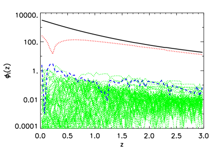

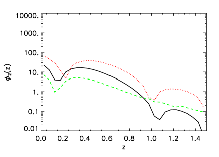
In Fig. 1 we plot as given in Eqn. (8) for the Planck experiment. The upper panel shows when cosmological parameters are fixed. In this panel, the first and second components are three orders of magnitude higher than the rest of . No sign transition occurs on the first mode, while on the second mode changes sign around . This is indicated by the kink in the logarithmic plot. In the lower panel we plot after the standard cosmological parameters have been marginalized. Compared with the upper panel, all are one order of magnitude smaller. This is due to the degeneracy between and the cosmological parameters, in particular .
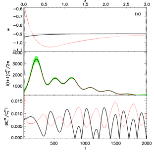
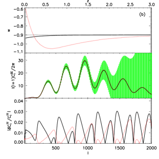
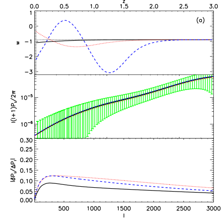
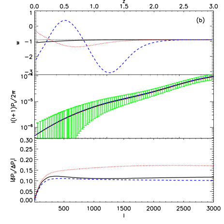
To visualize the impact of the principal component on the observable, we plot in Fig. 2 the change of when changes along the direction of the principal components, i.e, we construct as
| (10) |
where is the error on . For a data set with 60 parameters, give the 1- boundary along the -th eigenmode direction from the center. Note that the prefactor in this relation is there to represent a 1- errorbar in a 60-dimensional parameter space.
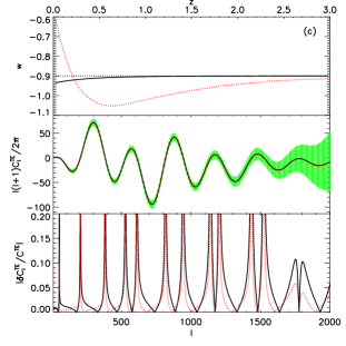
Figures 2 (a),(b) and (c) presents the changes of , and , respectively. The solid and dotted line represent changes in the first and second eigenmodes, respectively. In the top plot of each panel, we show how deviates from the fiducial value (faint dotted). For (solid), only deviates slightly from at ; while for (dotted), descends from at to around and then goes slowly back to at higher redshift. The second plot from the top in each panel shows how behaves. The light area shows the observational error. For every spectrum, the deviation from the fiducial is very small compared with the observational error, in fact too small to be seen in the graph. For clarity, we presents in the bottom plot in each panel the relative difference to show how changes. The peaks of have the same height, which indicates that shifts along when we add the principal components. This is because changes the expansion history of the Universe and therefore the angular positions of acoustic peaks. , and all have the same qualitative behaviour with changing eigenmodes. Notice in the bottom panel of (c) that the peaks become infinity because crosses zero at the same position.
The ‘constraint’ on from CMB power spectrum mainly come from the estimation on the angular positions of acoustic peaks. Since the angular positions also depend on , there is a large degeneracy between and (Bean & Melchiorri, 2002). Therefore, in the marginalized case is two orders of magnitude smaller than the one with fixed cosmological parameters. However, the first mode is still three orders of magnitude higher than the rest of . The second mode drops down two orders of magnitude, but it still changes sign around . The lower panel is consistent with the lowest panel of Fig.(1) in Crittenden & Pogosian (2005).
From the discussion above, one can tell that the information for from CMB power spectrum is very limited. However, since the Planck surveyor will be able to pin down the other cosmological parameters to a percentage level, we will choose it as a prior on cosmology when we evaluate from other dark energy probes.
4 Type Ia Supernovae
Type Ia SNe are so called standardisable candles and can be used to probe cosmological models (Perlmutter et al., 1999; Riess et al., 1998). Their luminosity distance-redshift relation provides a straightforward way to measure the expansion rate of the Universe. The magnitude-redshift relation for Type Ia SNe is given by
| (11) |
where is the apparent magnitude and is the intrinsic magnitude of the Supernovae. In order to forecast a given SNe survey, we have to choose a fiducial value for M, and we assume (Perlmutter et al., 1999). The luminosity distance in a flat Universe is given by
| (12) |
where is the speed of light and is the Hubble parameter. For a flat universe, is defined as
| (13) |
The Fisher matrix for the Supernovae survey is given by (Tegmark et al., 1998)
| (14) |
where is the density distribution of the Supernovae satisfying
| (15) |
where is the total number of SNe Ia in the survey, denotes the survey depth and is the error on the magnitude . We assume that for all Type Ia SNe surveys, which is a simplistic, but common assumption neglecting, for example, measurement errors and cadence differences.
We start our discussion with the SNAP survey (SNAP Collaboration, 2005; Albert et al., 2005). SNAP is a proposed space mission designed to measure the light curves and spectra of Type IA SNe and the spectra of their host galaxies to estimate their redshifts. It is estimated that up to SNe Ia could be found out between and , out of which will have well-measured light curves (SNAP Collaboration, 2005; Albert et al., 2005). Note that the value of in Eqn. (1) will be different depending on different survey parameters and for the SNAP SNe survey is .
For a flat Universe the only standard cosmological parameters relevant for Supernovae as cosmological probes are the total matter density and . The intrinsic magnitude can be combined with and be treated as a ‘nuisance’ parameter and marginalized over. However, we treat both of them separated given that can be constrained to a certain extent by the Planck surveyor.
We conservatively assume that we have calibration SNe Ia between . In addition, we assume that the rest of SNe Ia are uniformly distributed in redshift.
The evolution of the eigenmodes in , therefore, will mainly depend on the derivatives of the apparent magnitude with respect to . Fig. (3) shows all for this survey. There are eigenmodes in Fig. (3). As in the CMB case, we highlight the first three eigenmodes. The (black) solid line, the (red) dotted line and the (blue) dashed line represent , and , respectively. The faint (green) dotted lines show all higher order eigenmodes. The upper panel shows maintaining and fixed, while the lower panel represents the eigenvectors after marginalizing over and including the Planck prior. The errors on the components drop down linearly from the best constrained ones to the worst ones. By marginalizing over and , the amplitudes of become slightly smaller, which is consistent with the results of Huterer & Starkman (2003). We notice that the redshift dependence of the eigenmodes has changed with marginalization; the eigenmodes acquire zeros as we marginalize over and , indicating the impact of parameter degeneracies.
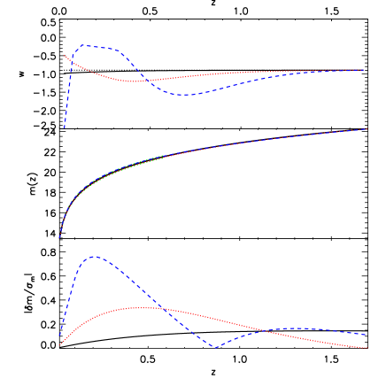
Fig. 4 shows how the apparent magnitude changes when changes along the direction of the eigenmodes. We take the first three components as examples. In the upper panel, we plot where for the 34 free parameters. The middle panel shows the magnitude . For clarity, we also show in the lower panel the absolute change relative to for each case. The solid line is when we vary the first eigenmode, while the dotted and dashed lines represent variations of the second and third eigenmodes, respectively. As we expect, the error on due to these variations is less than .
We can now proceed to compare the from SNAP, PS4 and DES SNe Ia surveys. PS4 will have a medium survey in the grizY bands over 1,200 deg2 and an ultra deep survey in the same bands over 28 deg2, which is two magnitudes deeper than the medium survey. These will allow potentially the detection of Type Ia SNe and in early type hosts333see at: pan-starrs.ifa.hawaii.edu/public/science/active.html. We note that DES and PAN-Starrs will not have the capability of spectroscopic follow-up. Therefore follow-up will have to be done with other instruments or photometric redshifts will have to be used. We do not consider these caveats in this analysis and assume real spectra are available for redshift determination. DES has a dedicated Supernovae program in conjunction with a spectroscopic follow-up for a sub-sample to test purity(The Dark Energy Survey Collaboration, 2005).
| Survey | N | redshift range | bins |
|---|---|---|---|
| DES | (0.3,0.75) | 15 | |
| PanStarrs-4 | (0.3,1) | 20 | |
| SNAP | (0.3,1.7) | 34 |
Table (LABEL:tb:expt_sne) lists the corresponding survey parameters and the number of bins that we use for each survey.
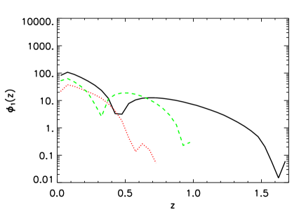
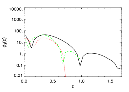
Fig. (5) shows and for each of these surveys. The solid , dotted and dash line indicate SNAP, DES and PS4, respectively. Given the state of current Supernovae surveys, DES, SNAP and PS4 will improve on the current situation by providing a very long exposure time on red filters, hence being able to find Supernovae at higher redshifts. We have not considered the PS1 Supernovae survey as it will not be considerably deeper in the red hence not providing much larger redshift coverage for the Supernovae detected, compared to current surveys. Due to the different distributions of the SNe and different minimum and maximum redshift, the eigenmodes peak in different locations. The relative amplitudes clearly show that surveys with more SNe Ia give better constraints, as expected and also found by Kim et al. (2004). On the other hand, DES and SNAP have a similar number of SNe Ia, but the constraint from DES is weaker because of its lower maximum redshift and its higher minimum redshift.
In reality, the SNe Ia distribution is unlikely to be constant; instead, is a result of the survey strategy. In order to find out how the depend on , we adopt a fiducial SNAP distribution given by Table(1) in Kim et al. (2004). Fig. (6) shows the with different assumptions on . The solid line in this plot represents by assuming constant , while the dotted line shows with the distribution from Kim et al. (2004). Beyond , the difference between these two cases is small. The amplitude of for the more realistic distribution is lower than the constant case due to a lower number of Type Ia SNe at low redshift. The peak of for the more realistic distribution is located at higher redshift.
5 Weak Lensing Tomography
Weak lensing tomography is a recent technique which assumes that light from distant galaxies travels to us in geodesics which are perturbed by the network of dark matter present in the Universe. These perturbations have the net result of changing the ellipticity of galaxies by roughly a per cent. By measuring the accurate shapes of galaxies and removing instrumental effects this cosmological effect is a nice probe of the growth of structure in our Universe (Hu, 1999). The techniques to extract the shear signal by looking at the ellipticities are vast and different for space based and ground based surveys (Heymans et. al., 2006; Massey et. al., 2007). Different surveys will differ mainly by the quality of their image, which will affect the quality of the shear measured, the quality of the photometric redshifts, which will be determined by the integration in each of the photometric bands and which will determine the ability to extract redshift information via tomography, and the total number of galaxies used for weak lensing which will be determined by a combination of the depth and the mean seeing of the survey.
Cosmology is extracted by the means of the weak lensing power spectrum. The weak lensing power spectrum is the weighted two-dimensional projection of the three-dimensional matter power spectrum, given by (Bartelmann & Schneider, 2001; Refregier et al., 2004)
| (16) |
where represents the pair of tomographic slices . is the comoving angular diameter distance given by
| (17) |
with from Eqn. (12). The upper limit of the integral represents the redshift of the survey depth. The window function is given by
| (18) |
where the weighting function represents the strength of the lensing signal for a source at a given redshift and a distribution of sources in each tomographic slice . Note that to distinguish the slice index form the -bin index, we use Greek letters to present the slice index in this section. is the matter power spectrum at redshift with representing the wavenumber for a given harmonic .
The Fisher Matrix for the weak lensing power spectrum is given by
| (19) |
with . Setting and , the elements of the covariance are given by (Ma et al., 2006)
in which is
| (21) |
which is a combination of the power spectrum and the noise. is the fraction of the sky coverage of the survey, is the shear variance due to the intrinsic ellipticity including other measurement errors. is the average surface density of galaxies. Eqn.(LABEL:eqn:cov_lens) holds under the Gaussian assumption on the convergence field. With , this approximation works very well (White & Hu, 2000; Cooray & Hu, 2001; Huterer & Takada, 2005). Therefore, in this paper, we take . The lowest is limited by the sky coverage of the survey. Also since the cosmic variance dominates at very low , low harmonics do not contribute much to the Fisher Matrix, we take the lower limit of .
One of the difficulties that we are facing in weak lensing tomography is to determine the matter power spectrum with the -binning parameterization. Dark energy modifies the growth of the matter perturbation and the shape of the matter power spectrum. The growth factor is analytically given by
| (22) |
with the prime representing the derivative with respect to the scale factor . However, since future weak lensing surveys extend to the nonlinear scale, the dependence of the shape of the nonlinear matter power spectrum on has to be considered when calculating the lensing power spectrum. Peacock & Dodds (1996) and Smith et al. (2003) developed a set of fitting formulae for calculating the nonlinear matter power spectrum with a cosmological constant assumption. Though work has also been done to correct the fitting formulae for constant (Ma et al., 1999; McDonald et al., 2006), this area is still limited to a non-evolving equation of state on a small cosmological parameter space. It requires a lot of effort calibrating the matter power spectrum considering evolving by running low resolution N-body simulations. However, since the aim of this paper is to demonstrate the behaviour of the eigenmodes of with different future weak lensing surveys, we simply generalize the method given by Smith et al. (2003) for -bin parameterization. We emphasize that in real data, either N-body simulation with evolving must be run or the non-linear must be predicted with a renormalisable perturbation theory model (Crocce & Scoccimarro, 2006) or run by a training set (Habib et al., 2007). Here we still use the fitting formulae in Smith et al. (2003) but use the transfer function ouput from modified CAMB code (see Sec.3).
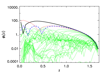
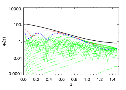
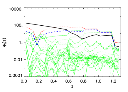
The SNAP weak lensing survey is one of the most representative future surveys. Its baseline is to image over square degree and approximately resolved galaxies will be found in one square arcmin (SNAP Collaboration, 2005) up to redshift . Six optical and three infrared filters are used to estimate the photometric redshift of the galaxies. In this paper, we adopt the simulated galaxy distributions in Refregier et al. (2004). We focus on the case with the three tomography slices since the constraint improves insignificantly with more slices. We set since SNAP can find galaxies up to redshift . Fig. (7) shows 60 . The (black) solid line represents . The (red) dotted line and (blue) dash line indicate and , respectively. The faint (green) dotted lines show all higher order modes. In the upper panel we fix the cosmological parameters. The first mode dominates at low redshifts and then decays along the redshift. Since the first mode drops down four orders of magnitude, at redshift , the second and third modes become dominant. The errors on the components drop down exponentially from the best constrained ones to those worst ones. In the lower panel, we show after cosmological parameters being marginalized including Planck prior. The amplitude of the first mode is slightly smaller in this plot. However the redshift dependences of the modes change dramatically. has a peak around . At redshift , there is less information from SNAP, so is mainly driven by Planck Prior. and are one order of magnitude lower than but still dominate at high redshift . This is consistent with Fig.(2) in Simpson & Bridle (2006) where they found that for cosmic shear, higher modes contributes significantly to weight function of .
To test how changes with the eigenmodes, we plot in Fig.(8) and its deviation from the fiducial value when we modify along the direction of the eigenmodes. The top plot on each panel shows , where for 60 free parameters. We choose the first three best estimated modes after marginalization as the examples which are represented by (black) solid, (red) dotted and (blue) dash lines, respectively. In the second plot of the left panel, we show the auto correlation of the first slice, i.e. with . The second plot of the right panel shows the cross correlation between the first slice and second slice, i.e. with . The light shaded area is the error around the fiducial value which is presented as the black solid line. For clarity, we show in the bottom the absolute change of relative to the error bar for each mode. The deviation is very small compared with the error bar, which shows that the first three modes are well constrained. However, the error in this plot only comes from a single shell. One also obtains constraints on from other auto and cross correlations.
In the following of this Section, we compare SNAP with four other weak lensing surveys: EUCLID, DES, PS1 and PS4. SNAP and EUCLID are space based, while DES and PS (1 and 4) are ground based surveys. As stated before ground based surveys and space based surveys have different systematic effects which enter the weak lensing analysis. Image quality in space is far superior than on the ground. This will allow for better shape measurements in space. This effect is hard to include in a Fisher analysis. we would be able to include this effect by producing image simulation and estimating what and we would have for a given seeing and magnitude depth. Producing image simulation is beyond this work, so we simply keep roughly constant and change to take account for the effects of image quality. The other main difference is the seeing. Even though PS4 will probe the sky to greater depths than EUCLID or SNAP, it will have less galaxies usable for weak lensing as the seeing lowers the surface brightness of sources and many faint galaxies fall below the signal to noise required for a detection. These differences are encoded within Table.(3) which lists the experiment parameters. To calculate the lensing power spectrum, one has to know the galaxy distribution. Since all these four surveys will use photometric redshifts, one has to take into account the photometric redshift errors . A more common method to include is analytical convolution of the galaxy distribution with the probability distribution function of the photo-z (Ma et al., 2006). For simplicity, is assumed to be Gaussian with scatter and bias . In this paper, we use mock photometric catalogues to calculate for each tomographic slice. These photometric catalogues have been produced in the following way: galaxies from GOODS have been cloned and their photometry has been calculated analytically. Then we have used a photometric redshift code to estimate the photo-z for these galaxies having set aside a given number of galaxies for training purposes. A more detailed discussion regarding the creation of these mocks can be found in Abdalla et al. (2007) and Banerji et al. (2007). Based on these catalogues, we choose five slices for EUCLID and PS4, three slices for DES and PS1. We also list for each in Table.(3).
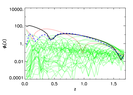
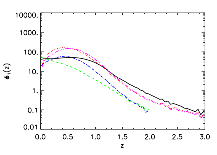
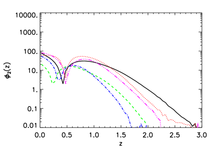
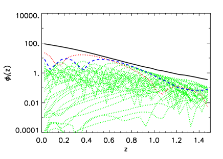
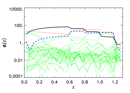
We plot (upper panel) and (lower panel) in Fig. (9). We marginalize the Fisher matrices over the cosmological parameters and including a Planck prior. As we expect, of DES (green dashed) and PS1 (blue dash-dotted) are about one order of magnitude lower than of SNAP (black solid), EUCLID (red dotted) and PS4 (magenta dash-tripled-dotted). DES has a relatively small sky coverage and number density of galaxies. PS1 covers half the survey, but has a relatively small number density of galaxies. The redshift dependences of are different as well. of DES decays along the redshift; this may be due to the fact that the values of the intrinsic Fisher matrix of DES is small so that the Planck priors have a bigger effect in the analysis. of the rest peak around but stays positive in the whole redshift region. We notice that the redshift dependence of do not change much for different surveys except for the amplitudes and the redshift where . We also found that with a Planck prior, depend weakly on how we define the tomographic slices.
If we compare the eigenmodes between DES and PS1, one can also notice that PS1 has better constrained eigenmodes than DES. Among SNAP, EUCLID and PS4, EUCLID and PS4 have better constraints on the eigenmodes than SNAP. Amara & Réfrégier (2007) conclude that the sky coverage is the dominant parameter on improving the figure of merit rather than and .
| Survey | |||||
|---|---|---|---|---|---|
| SNAP | 0.024 | 1.23 | 3 | ||
| EUCLID | 0.5 | 0.83 | 3 | ||
| DES | 0.12 | 0.67 | 2 | ||
| PS1 | 0.6 | 2 | |||
| PS4 | 0.83 | 3 |
6 Galaxy Cluster Counts
Galaxy cluster counts probe cosmological models via the redshift dependence of the survey volume and the sensitivity of the halo mass function to the linear growth of structures. Forthcoming galaxy cluster counts will be performed by selecting clusters via their Sunyaev-Zel’dovich decrement, for example with Planck (ESA-SCI(2005)1, 2005) or the South Pole Telescope (Ruhl et al., 2004) or in the x-rays with, for example, the extended ROentgen Survey with an Imaging Telescope Array (eROSITA)444see at: http://www.mpe-garching.mpg.de/projects.html#erosita. Finally future imaging and photometric redshift surveys will be able to identify clusters in the optical wavebands (Koester et al., 2007; Rozo et al., 2007). For example DES and EUCLID would be able to identify thousands of clusters with this method.
The redshift evolution of the number of the clusters in the redshift interval between and found by a Galaxy Cluster survey is given by
| (23) |
where is the sky coverage. is the comoving volume element, is the mass limit above which clusters can be found at redshift for a given set of survey parameters. is the number density of the clusters with mass and redshift ; in this paper we adopt the fitting function of presented by Jenkins et al. (2001)
| (24) |
where is the matter density at present, is the growth factor is the linear overdensity at mass scale at redshift , which is given by
| (25) |
where . We use a spherical top hat window function
| (26) |
The last term is the linear power spectrum . Following Sec.(5), we use CAMB to calculate the transfer function and the power spectrum .
The Fisher matrix for the cluster counts is given by (Haiman et al., 2001; Levine et al., 2002)
| (27) |
In which is the number of clusters in redshift interval at redshift , with the maximum redshift of the survey.
In order to extract cosmology from a galaxy cluster count survey we need to understand the relation between the survey parameters and the limiting mass of the survey. For example for Sunyaev-Zel’dovich cluster surveys, is a function of the flux limit at frequency (Battye & Weller, 2003). In this context to estimate , one requires well-calibrated mass-temperature relation for galaxy clusters and an understanding of the scatter (Lima & Hu, 2004). However in order to get an estimate of the ability of galaxy cluster counts to constrain the equation of state for different types of cluster selection, we assume a limiting mass, which is constant in redshift and neglect scatter. It is straight forward to include scatter in any analysis however it is not clear at the moment how large the intrinsic scatter is for different survey strategies.
The South Pole Telescope (SPT) is a bolometric array observing 4,000 square degree of the southern sky in 3-4 radio wavebands, with the main signal coming from the 150GHz channel. It will discover thousands of cluster roughly above a mass threshold of . The Dark Energy Survey is observing the same area of sky as SPT and will provide photometric redshifts and vital weak lensing information for the the galaxy clusters. The observed redshift range goes roughly out to . In Fig.(10) we show for fixed and marginalized cosmological parameters. As before we highlight the first three components. We find that only the first eigenmode is dominating. This is similar to the SNe case, where the hierarchy of modes is almost linear. After we marginalize over the other cosmological parameters, the amplitudes of the eigenmodes are one order of magnitude lower. Notice that the eigenmodes do not change significantly after the marginalization. This is because we impose the prior from Planck, which constrains the other cosmological parameters very tightly.
In order to test the significance of the eigenmodes, we replace the fiducial model of with with corresponding to the errorbars for 30 free parameters. In Fig. (11), we plot for the fiducial model and when for the first three modes. The solid, dotted and dashed lines represent modes , respectively. In the top panel, we show . In the second panel from the top, we show together with Poisson errors around the fiducial model (faint dotted). For clarity, we show the absolute change relative to the error bar in the lowest panel. For some redshifts where , is larger than expected for the third eigenmode indicating that there might be redshift ranges where we can constrain up to three modes, although overall the constraint on this mode is much weaker than the on the first eigenmode. This agrees with earlier findings (Battye & Weller, 2003) that cluster counts will be able to give a good constraint on since can affect both the volume element and the growth factor .
In order to compare different surveys we show in Fig. (12) and for three different cluster surveys with mass limits of (solid), (dotted), (dashed), all over 4,000 deg2 out to a maximum redshift of . The lower mass limit could correspond to optical cluster selection like DES or EUCLID, albeit any realistic treatment should include scatter in the mass limit for these surveys. Nevertheless we clearly see that a lower mass limit leads to much better determined modes, due to the fact the number of observed cluster increases dramatically for lower mass limits.
7 Baryon Acoustic Oscillations
Baryon Acoustic Oscillation (BAO) arise from the fluctuation due to the sound waves in the plasma which was composed of tightly coupled CMB photons and baryons before recombination. After combination, photons decoupled from baryons; thereafter the acoustic waves were imprinted as fluctuation in the density fields of both photons and baryons. Though baryons followed the structure evolution of the underlying dark matter field, the spatial scale of the acoustic oscillation is well reserved as a standard ruler which can be used to calibrate the geographical evolution of the Universe. As galaxies are tracers of baryons, galaxy redshift surveys have been performed to be a complementary probe to constrain cosmological parameters and the properties of dark energy (Percival et al., 2007).
The basic idea of BAO is to calibrate the length scale of the acoustic waves at different redshifts and fit this distance-redshift relation with cosmological models. The numerical details of the methodology vary according to different authors. In this paper, we use the methodology developed in Seo & Eisenstein (2003), where the full matter power spectrum has been used to measure Hubble parameter and the angular diameter distance given by
| (28) |
is estimated from galaxies in a redshift shell centered at . The fisher matrix at the shell is given by (Seo & Eisenstein, 2003)
| (29) |
where is the norm of the wave vector , is the cosine of the angle between and the line of sight. is the effective volume of the redshift shell given by
| (30) |
in which is the vector along the line of sight and is the comoving number density of the galaxies.
The observed power spectrum in Eqn. (29) is given by (Seo & Eisenstein, 2003)
| (31) | |||||
in which and present the traverse and line-of-sight directions, respectively. The index “ref” indicates the reference cosmology we use. In this paper, we set the reference cosmology the same as the fiducial model that we assume. is the shot noise power. is the bias factor and is . We treat the bias of each shell independently as an nuisance parameter and marginalize over them in the analysis. In reality, the fiducial value of the bias depends on galaxy types that one uses to recover the power spectrum. Here we assume for all galaxy surveys expect for the SKA, where we assume .
One uncertainty in Eqn. (29) is the upper integral limit of . This has been discussed by different authors (Blake & Glazebrook, 2003; Seo & Eisenstein, 2003). In this paper, we choose a conservative value of for shells at where most surveys reach. For WFMOS deep, we choose , as it is a much higher redshift survey and will probably have non-linearity which will prevent us to measure for larger .
For spectroscopic galaxy surveys, if we ignore the correlation between the shells for very small along the line of sight, the Fisher matrix of the whole survey can be obtained simply by adding together the Fisher matrices at different redshift shells. However, one has to be careful with the photometric redshift surveys. The relative large photo-z error will smear the power spectrum along the line of sight and introduce a cross correlation between different shells. In this paper we ignore the cross correlation between different shells, but given that the photo-z damps the power spectrum along the line of slight, i.e.
| (32) |
where is taken from simulations (Abdalla et al., 2007). We choose the width of the shells to be much larger than the photo-z error of galaxies in that shell. This strategy is also a solution for avoiding the cross correlation between shells (Seo & Eisenstein, 2003).
Another freedom in the analysis is how to choose the redshift shells. The principle is to make sure that the width is large enough that one can measure two or three wiggles in the power spectrum along the line of sight in that shell. At the same time, we wish to make the shell thin enough so that we have enough information for at each bin. Therefore a choice of as the shell width means reasonable for most surveys. For WFMOS deep, we use (see Table.(LABEL:tb:bao_slice)).
| Survey | redshift range | ||
|---|---|---|---|
| WFMOS(wide) | 0.05 | ||
| WFMOS(deep) | 0.0075 | ||
| SKA | (0.,2) | 0.5 |
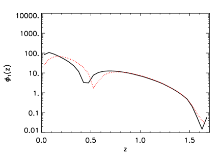
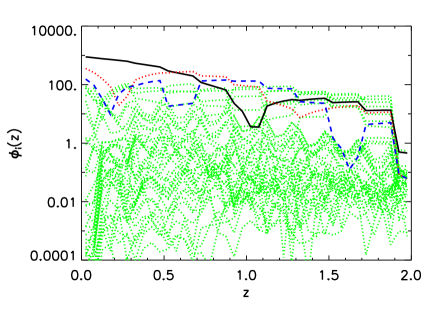
Two out of the three surveys planned by WFMOS (“wide” and “deep”) will provide a competitive constraint on cosmology and dark energy (Glazebrook et al., 2005). In this section, we take the wide survey as an example and study how behaves in this case. Table.(LABEL:tb:expt_bao) shows the parameters for WFMOS survey and in Table.(LABEL:tb:bao_slice) the locations of the slices. We use -bins for . We plot in Fig. (13). The (black) solid line indicates the best estimated eigenmode. The (red) dotted line and (blue) dash line indicate the second and the third eigenmode, respectively. The (green) dotted lines show the other eigenmodes. In the upper panel we marginalize over the biases of each of the shells. The first mode dominates at low redshift but decays slightly along and crosses zero around . At redshift , the second and third modes dominate. In the lower panel, we show after marginalization over all other parameters including a Planck prior. In this plot the first eigenmode peaks around where the survey starts. In both panels, the value of is still significant, which is different from other probes. This is also consistent with Simpson & Bridle (2006) where they found that the weight function of BAO shows a high sensitivity on at high redshift due to the location of the data at high redshift. The second and third modes are also significant at high redshift. The obvious discontinuity are found at the redshift where the shells are located.
| Survey | 1 | 2 | 3 | 4 |
|---|---|---|---|---|
| WFMOS(wide) | 0.6 | 0.8 | 1.0 | 1.2 |
| WFMOS(deep) | 2.5 | 3.0 |
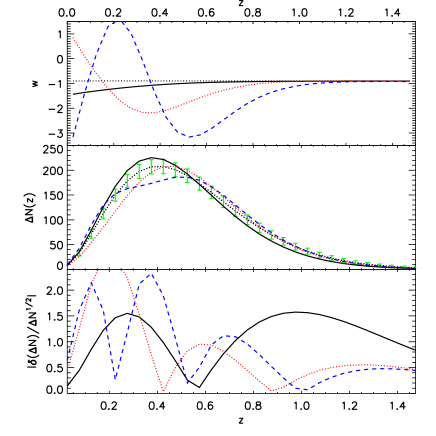
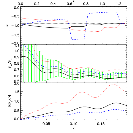
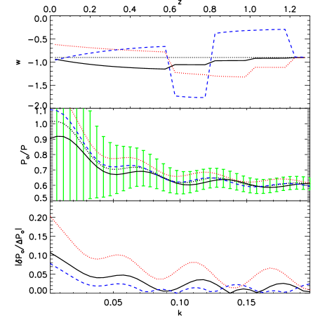
In Fig. (14), we show how changes along with . We take the first redshift shell in WFMOS wide survey as an example. The left panel shows the power spectrum perpendicular to the direction of the line of sight which corresponds to , while the right panel shows the power spectrum along the line of sight which corresponds to . In all the panels, the (black) solid line indicates the first eigenmode. The (red) dotted line and the (blue) dashed line represents the second and third modes, respectively. The top plot on each panel shows , where for . Here we use shown in the lower panel of Fig. (13). One can notice that deviates from the fiducial values dramatically at high redshift, which is different from what we found from SNe Ia, WL and Cluster Count. The second plot from the top presents the divided by the power spectrum without baryons and normalized to the same value at . The (green) error bars represent the error on the power spectrum, which is given by (Seo & Eisenstein, 2003)
| (33) |
In order to be consistent, we also divide by the fiducial power spectrum without baryons. In the bottom plot we show the absolute change relative to the error bar. As we expect, is smaller than the error of the power spectrum. One can also notice that the amplitude of the power spectrums changes significantly compared with the scale of the wiggle.
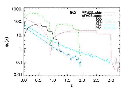
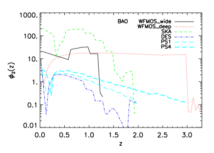
In Fig. (15), we show and from different redshift surveys marginalized with Plank prior. There are seven surveys shown in this plot. The (black) solid line indicates WFMOS wide; the (red) dotted line represents WFMOS deep. The (green) dash line represents SKA. Note that we have not analysed EUCLID BAOs in this paper, which is a strong component of the EUCLID program. Because of the large cosmic volume, the height of for the SKA is one magnitude larger than for other surveys. For WFMOS deep, the data comes from redshift ; therefore dominates at high redshift. However, is significant at very low redshift as well. Both of SKA and WFMOS deep cross zero around , which is different from of WFMOS wide. Besides WFMOS and SKA, we also show the eigenmodes from photo-z redshift surveys. The (blue) dash dotted line shows DES, the (cyan) thin long dash line shows PS1 and the thick one represents PS4. These ’s are very similar to from Planck prior. This is because of the damping factor on the power spectrum of the line of sight due to the photo-z error. The values of the Fisher matrices are relatively small compared with Planck prior; therefore the Planck prior has a larger effect on .
8 Joint Principal Components
We have performed PCA analysis on a few representative future surveys. In the following, we will compare the eigenmodes for different stages and discuss the joint principal components from each stage. All the probes discussed in this section are marginalized over the other parameters including the Planck prior.
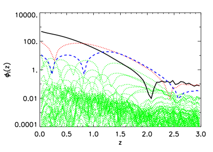
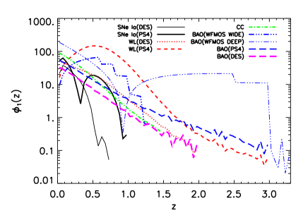
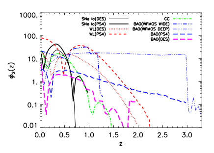
In Fig. (16), we show (upper panel) and (lower panel) for the surveys that we have analysed for stage III . The (black) solid line indicates SNe Ia surveys with the thin and thick lines representing DES and PS4, respectively. The (red) dotted and dash lines represents WL from DES and PS4, respectively. The (green) dash-dotted line shows the cluster count result. The remaining lines show the result for BAO surveys; the (blue) long dashed line is for PS4 and the (magenta) thick long dash line represents DES. The (blue) dash triple-dotted lines show WFMOS with the thin and thick lines representing deep and wide, respectively. The amplitudes of for this stage are roughly between ten and one hundred. of PS4 for WL dominates at redshift ; while of WFMOS deep for BAO is dominant for higher redshifts. The redshift dependence of can be classified into three types. First, behaves very similar to the first mode of the Planck prior, which is represented by CC and BAO from DES and PS4. This is due to the relatively strong Planck prior for these cases. Second, crosses zero at low redshift. of DES and PS4 for SNe Ia and WFMOS deep for BAO show this feature. However for WFMOS deep this feature is already at intermediate redshifts around . The third type of behaviour is encountered by PS4 for WL and WFMOS wide for BAO. stays positive and peaks at the median redshift. For most of the probes, is significant at low redshift and then decays afterward, while WFMOS deep has also a very significant contribution at high redshift above . In the lower panel, we notice that the amplitude of the second mode is already one order of magnitude lower than the first mode. The dominant contribution of is still at low redshift, with the exception of WFMOS deep. Due to the dominance of the first mode the main redshift dependence of a given survey is encoded in this mode (Huterer & Starkman, 2003).
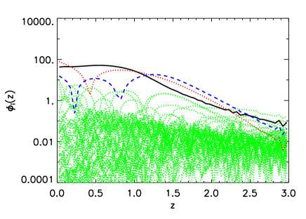
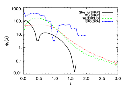
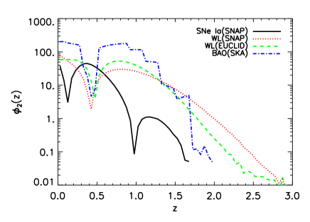
Fig. (17) shows the two leading modes for the stage IV surveys in our analysis. The (black) solid line is for type Ia SNe from SNAP. The (red) dotted line shows WL from SNAP and the (green) dash line shows WL from EUCLID. The (blue) dash dotted line shows BAO from SKA. The amplitudes of for this stage are about one order of magnitude higher than in stage III; SKA for BAO dominates in its redshift range . of SNAP for SNe Ia and BAO for SKA have a change in sign for the most dominant mode, while of both SNAP and EUCLID for WL have a mode which stays positive throughout. The amplitude of is about one order of magnitude lower, hence of the same significance as the primary mode for the stage III surveys.
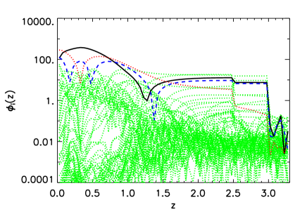
From the four probes that we discussed, one can find that for most surveys the best constrained eigenmodes dominate at low redshift. The exception are surveys which target objects at high redshifts as for example WFMOS deep. from WFMOS deep stands out at high redshift in the upper panel of Fig. (16). In the following, we discuss how the eigenmodes behave if we combine different probes. We perform the joint analysis based on the two stages. For stage III, we combine PS4(SNe Ia), PS4(WL) and WFMOS deep (BAO). For stage IV, we combine SNAP(SNe Ia), EUCLID(WL) and SKA(BAO). We also include the Planck prior for both cases. In Fig. (18) we show the joint eigenmodes with the upper panel and the lower panel representing the Stage III and IV, respectively. We find that is significant within the whole redshift range expect around where changes sign. It is interesting to note that higher order modes and namely the second mode fill this gap in redshift. In addition boosting at high redshift, WFMOS deep (BAO) is complementary with PS4(SNe Ia), PS4(WL) at high redshifts. For Stage IV we find that the equation of state will be constrained significantly at least out to redshift .
9 Reconstruction
So far, we have compared different surveys by concentrating on the behaviour of and , which allows us to explore the redshift sensitivity on for each probe. To reconstruct , however, one would like to include higher order eigenmodes to get less bias in the reconstructed equation of state. However, if we use higher order eigenmodes the error on the reconstructed is dominated by the errors from these orders. In order to decide how many eigenmodes to use for reconstruction we require the bias and the variance to be low. Hence, an alternative to the standard figure of merit of a survey (Albrecht et al., 2006) is to count how many eigenmodes can be well constrained under a certain criteria.
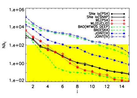
In Fig. (19), we plot the first 15 eigenvalues weighted by the number of bins, for the different surveys that we used in the joint analysis in the previous section. All the surveys are marginalized over other parameters including Planck priors. The (black) solid line shows the Type Ia SNe surveys with the filled and unfilled circles indicating PS4 and SNAP, respectively. The (red) dotted lines represents the WL surveys, with the filled and unfilled stars indicating PS4 and EUCLID, respectively. The (green) dashed lines represents the BAO surveys with the filled and unfilled triangles indicating WFMOS deep and SKA, respectively. We also show the joint analysis with the (blue) dotted-dash lines; the filled and unfilled squares indicating stage III and IV, respectively.
In order to explore the problem of the w-reconstruction quantitatively let us assume that one only uses eigenmodes. The reconstructed is then given by
| (34) |
where is the value around we wish to reconstruct the equation of state. The are the best fit coefficients in the eigenmode basis . The reconstruction strategy given by Huterer & Starkman (2003) is equivalent to setting and the expected is then given as the projection of on the fiducial model. Crittenden & Pogosian (2005) define under the assumption that is close to the true physical model for any reconstruction in a real data situation and in this case the expected are zero.
We now have to employ a statistical criterion, which allows us to gauge how many eigenmodes to use for the reconstruction of the equation of state. There are three effects at work, which need to be considered. First the goodness of the fit, which, of course, improves with the number of used modes, second the degradation of the errorbars with increasing number of modes and finally the bias between the true underlying model and the model, , around which we reconstruct the equation of state. As we will show below the Bayes’ factor (Jeffreys, 1939; Trotta, 2008) based on Bayesian evidence (Sivia, 1996) provides exactly such a criterion.
We will proceed by describing a Gaussian approximation of the Bayes’ factor, based on Bayesian evidence, to decide the number of significant modes. We will follow closely the discussion in Saini et al. (2004). Under Gaussian assumptions, which hold for the Fisher matrix approximation of the underlying likelihoods, the evidence for the data given the hypotheses H is approximated by
| (35) |
with the covariance between the w-bin parameters, , in the basis of the eigenmodes, the covariance of the prior on these parameters and are the parameters of the maximum likelihood. is the term which encodes the overlap of the prior with the likelihood, i.e. this term is measuring the bias between the prior and the likelihood and is given by
| (36) |
where is the mean of the prior, which we choose to be or in the expansion given in Eqn. 34. If we make the simplistic assumption that the prior is diagonal and the same in each bin we obtain
| (37) |
Note that this prior, because of its diagonal nature, has the same form in the original w-bin basis and the eigenmode basis. Here we have to make an important point. We would like that the rms variance, , on the mean equation state for the prior is independent of the number of bins. Hence we have to scale the error in each bin, according to
| (38) |
Finally we will assume that the maximum likelihood can be written as
| (39) |
We will introduce the index to define the evidence for modes. Keeping in mind that we work in the basis where the entries in the covariance matrix are given by the eigenvalues we can write the evidence for modes as
| (40) | |||||
where the first terms measure the ’goodness-of-fit’ of the M modes, the second term the overlap between the prior and the likelihood and the last term is Occam’s razor by comparing the posterior to the prior volume. We can now construct the Bayes’ factor (Jeffreys, 1939; Trotta, 2008)
| (41) | |||||
where and are the the log-likelihood values at the best fit points, if we fit for or modes respectively. and are the best fit expansion parameters for these two cases.
We will first discuss the simple case with no bias. In this case we choose . Since we are expanding around the fiducial model we obtain for all expansion coefficients . Since there is no difference between ignoring modes or putting the best fit likelihood between and modes is exactly same, i.e. . Hence both the best fit and the overlap term vanish for the Bayes’ factor and only Occam’s razor term remains. If we further assume the prior is wide compared to the likelihood we obtain for the Bayes’ factor
| (42) |
Hence, in this approximate scenario the evidence ratio is given by the ratio of the likelihood uncertainty on the st mode, , to the prior uncertainty on a single bin . Although the equation of state at low redshifts is determined almost to the 10% level by current data, it is much more uncertain at higher redshifts. We hence choose for the rms uncertainty on the mean averaged over the entire redshift range. According to Jeffrey’s scale (Jeffreys, 1939) we have strong evidence if the Bayes’ factor is 1-2 and substantial evidence if it is between 0.5 and 1. We choose 1 as our evidence level. If we employ this we find as a condition for strong evidence
| (43) |
The shaded region in Fig. 19 highlights the area where this condition is violated. All points above the shaded region are eigenmodes, which are significant. We obviously find that the joint analysis can determine more higher order eigenmodes than the individual surveys, which is consistent with Fig. (1) in Crittenden & Pogosian (2005). This comes from the complementarity of the different dark energy probes. For most of the probes, the eigenvalues descend exponentially.
We will now continue to analyse the full Bayes’ factor expression in Eqn. 41 to decide for how many eigenmodes we have strong evidence. We will discuss two cases: As before the unbiased case where we reconstruct the equation of state around the fiducial model and a biased case where we choose . The latter is what will happen in a realistic situation, where the true underlying model is not known a priori, although one could imagine an iterative method to end up reconstructing around the true underlying model, but this is a posterior statement.
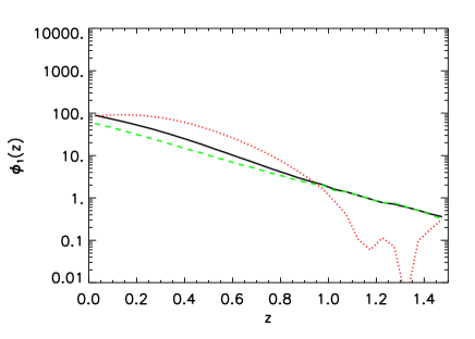
To illustrate how will take effect on the reconstruction, we give a very simple example for the SNAP SNe Ia survey. We take the eigenmodes from the SNAP SNe Ia survey with fixed cosmological parameters and use our fiducial cosmology with . In Fig. (20) we plot the reconstructed for different and . The solid line is for and the dotted and dash lines for and , respectively. The thin (black) lines are for and (blue) thick lines represent . One notices that no matter how we choose , will be around the fiducial model at low redshift, while at high redshift, will be biased towards . This is because SNe Ia surveys have very weak constraints on at high redshift.
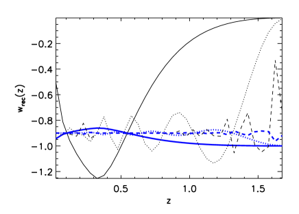
Fig. (20) also shows the oscillation on at high redshift, which is an artifact of the PCA decomposition. This is due to the limited number eigenmodes with that we choose to reconstruct with. For , has no constant behaviour with redshift. As we include more eigenmodes, starts to converge around for redshifts . The oscillation at high redshift are consistent with the results in Huterer & Starkman (2003), in which the analysis indicates that it is not possible to recover at redshift with SNAP SNe data. It is hence important to keep in mind the redshift evolution of the eigenmodes for the interpretation of the reconstructed equation of state. This simple example indicates that the choice of will make a difference for the reconstructed . If we compare the curves with , we find that the thin line starts oscillating around , while the (blue) thick line starts oscillating at around . The dashed lines which show the behaviour if we include modes, both the thin line and the (blue) thick line start oscillating at . However, the amplitude of the latter is much smaller indicating that our initial guess value is much closer to the true fiducial model. Huterer & Starkman (2003) use a mean square error (MSE) criteria to find the optimal number of modes, which minimize bias and variance simultaneously. However this criteria does not include an Occam’s razor factor by comparison to the prior information. Crittenden & Pogosian (2005) use a similar MSE, but include the prior variance. However their reconstruction is unbiased and they do not use MSE to decide on the number of significant modes, they use MSE over all modes to compare the effectiveness of different probes. As stated above we will use the Bayes’ factor to compare how many modes are significantly constraint for different probes. We believe that the measure provided by MSE of both Huterer & Starkman (2003) and Crittenden & Pogosian (2005) is included in our evidence expression and incorporates both principles. Although the Jeffrey’s scale is to some extend arbitrary we can clearly identify for how many modes there is strong evidence and for which modes there is only marginal evidence for different surveys.
| Expt. | SNe Ia | WL | CC | BAO | Joint |
| DES | 2(3) | 1(3) | 1(2) | 1(2) | |
| PS1 | - | 2(3) | - | 1(2) | |
| WFMOS(WIDE) | - | - | - | 3(3) | |
| WFMOS(DEEP) | - | - | - | 2(4) | |
| PS4 | 2(5) | 3(3) | - | 1(2) | |
| EUCLID | - | 3(4) | - | * | |
| SNAP | 2(5) | 2(3) | - | - | |
| SKA | - | - | - | 10(9) | |
| Joint III | - | - | - | 6(8) | |
| Joint IV | - | - | - | 12(12) |
In Table 6, we show the number of modes with strong evidence for the unbiased case and in brackets for the biased case. Note that in general the number of modes for the biased case are larger, although there are exceptions. For each survey, we include a Planck prior on the cosmological parameters. For most surveys, is around except for SKA. With the joint analysis, will be about for stage III, which indicates the complementarity of the probes; for stage IV, is , which is mainly driven by SKA.
10 Conclusions
In this paper we have studied future constraints on -bins for four dark energy probes, Type Ia Supernovae, weak lensing, cluster counts and baryon acoustic oscillations.
Instead of assuming that the equation of state parameter can be modeled by a simple function with a few parameters, we bin given by Eqn. (1) and treat each as independent parameter. Throughout this article, we choose fixed to make sure that we can compare between different surveys. For each probe, we choose a few representative future surveys. We also use a prior from the forthcoming Planck CMB experiment as prior on all remaining cosmological parameters. We find that in future mainly weak lensing and BAO surveys are complementary, in a sense that weak lensing gives tight constrain at low redshifts but BAO allows one to push to higher redshifts. However the role of Supernovae is also complementary for low redshifts. The high redshift sensitivity of the BAO would allow one to study also early dark energy models (Caldwell et al., 2003) in an efficient way. However at lower redshift weak lensing and Supernovae are the more efficient probes, with the exception of SKA BAO measurements. Typically forthcoming surveys constrain 2-3 modes. Since it is likely that there will be a multiple of stage III probes it is sensible to look at the combined power of these probes and we find that in this case five modes would be constraint. We would advocate that the number of well constraint modes is actually a better figure of merit than the one put forward by the DETF, since it encompasses the ability of future surveys not just to measure the equation of state at two redshifts, today and at the pivot point. We address the question of the number of modes in a Bayesian model selection way (Saini et al., 2004; Liddle, 2004). Although this method has recently attracted some criticism (Efstathiou, 2008) it provides a well defined framework to establish the significant number of modes for a particular survey. It takes into account the goodness of fit, the bias and Occam’s razor. However it is not only important to establish the significant number of modes. In addition the redshift distribution of the significant modes has to be taken into consideration to start talking about the complementarity of surveys. The complementarity can than be exploited to constrain eight modes for the joint stage III probes and twelve for stage IV if we include SKA. One question we have not addressed in this paper is how useful surveys are to probe “dark energy” beyond the background evolution, for example by probing structure formation. It is likely that in this context future weak lensing, and to some extend galaxy cluster surveys, will play a pivotal role. To conclude we would argue that all four discussed probes have their merits, but weak lensing and baryon acoustic oscillation surveys seem to bear the largest promise for revealing the nature of the accelerated expansion of the Universe.
Acknowledgments
We gratefully thank Peter Capak and Huan Lin for kindly providing us with simulation data. We sincerely thank Nick Kaiser for providing us information related to Pan-Starrs 1. We acknowledge Sarah Bridle, Rob Crittenden, Joshua Frieman, Gert Hütsi, Ofer Lahav and Antony Lewis for very helpful discussions.
References
- Abdalla et al. (2007) Abdalla F. B., Amara A., Capak P., Cypriano E. S., Lahav O., Rhodes J., 2007, ArXiv e-prints, 705
- Abdalla & Rawlings (2005) Abdalla F. B., Rawlings S., 2005, MNRAS, 360, 27
- Abdalla & Rawlings (2007) Abdalla F. B., Rawlings S., 2007, MNRAS, 381, 1313
- Albert et al. (2005) Albert J., et al., 2005, astro-ph/0507460
- Albrecht & Bernstein (2007) Albrecht A., Bernstein G., 2007, Phys. Rev. D, 75, 103003
- Albrecht et al. (2006) Albrecht A., Bernstein G., Cahn R., Freedman W. L., Hewitt J., Hu W., Huth J., Kamionkowski M., Kolb E. W., Knox L., Mather J. C., Staggs S., Suntzeff N. B., 2006, astro-ph/0609591
- Albrecht & Skordis (2000) Albrecht A., Skordis C., 2000, Physical Review Letters, 84, 2076
- Allen et al. (2004) Allen S. W., Schmidt R. W., Ebeling H., Fabian A. C., van Speybroeck L., 2004, MNRAS, p. 258
- Amara & Réfrégier (2007) Amara A., Réfrégier A., 2007, MNRAS, 381, 1018
- Astier et al. (2006) Astier P., et al., 2006, A.&Ap., 447, 31
- Banerji et al. (2007) Banerji M., Abdalla F. B., Lahav O., Lin H., 2007, ArXiv e-prints, 711
- Bartelmann & Schneider (2001) Bartelmann M., Schneider P., 2001, Physics Report, 340, 291
- Battye et al. (1999) Battye R. A., Bucher M., Spergel D., 1999, ArXiv Astrophysics e-prints
- Battye & Moss (2005) Battye R. A., Moss A., 2005, Journal of Cosmology and Astro-Particle Physics, 6, 1
- Battye & Weller (2003) Battye R. A., Weller J., 2003, Phys. Rev. D, 68, 083506
- Bean & Melchiorri (2002) Bean R., Melchiorri A., 2002, Phys. Rev., D65, 041302
- Blake & Glazebrook (2003) Blake C., Glazebrook K., 2003, Astrophys. J., 594, 665
- Blake et al. (2004) Blake C. A., Abdalla F. B., Bridle S. L., Rawlings S., 2004, New Astronomy Review, 48, 1063
- Bousso (2006) Bousso R., 2006, ArXiv High Energy Physics - Theory e-prints
- Buchert (2005) Buchert T., 2005, Classical and Quantum Gravity, 22, L113
- Caldwell & Doran (2005) Caldwell R. R., Doran M., 2005, Phys. Rev. D, 72, 043527
- Caldwell et al. (2003) Caldwell R. R., Doran M., Müller C. M., Schäfer G., Wetterich C., 2003, ApJ, 591, L75
- Carilli & Rawlings (2004) Carilli C., Rawlings S., 2004, ArXiv Astrophysics e-prints
- Carroll et al. (2004) Carroll S. M., Duvvuri V., Trodden M., Turner M. S., 2004, Phys. Rev. D, 70, 043528
- Carroll et al. (2005) Carroll S. M., et al., 2005, Phys. Rev. D, 71, 063513
- Chevallier & Polarski (2001) Chevallier M., Polarski D., 2001, International Journal of Modern Physics D, 10, 213
- Cimatti et al. (2008) Cimatti A., Robberto M., Baugh C. M., Beckwith S. V. W., Content R., Daddi E., De Lucia G., Garilli B., Guzzo L., Kauffmann G., Lehnert M., Maccagni D., Martinez-Sansigre A., Pasian F., the SPACE team 2008, ArXiv e-prints, 804
- Cline et al. (2007) Cline J. M., Frey A. R., Holder G., 2007, ArXiv e-prints, 709
- Cole et al. (2005) Cole S., et al., 2005, MNRAS, 362, 505
- Cooray & Hu (2001) Cooray A., Hu W., 2001, ApJ, 554, 56
- Crittenden & Pogosian (2005) Crittenden R. G., Pogosian L., 2005, ArXiv Astrophysics e-prints
- Crocce & Scoccimarro (2006) Crocce M., Scoccimarro R., 2006, Phys. Rev. D, 73, 063519
- De Felice et al. (2006) De Felice A., Hindmarsh M., Trodden M., 2006, Journal of Cosmology and Astro-Particle Physics
- de Putter & Linder (2007) de Putter R., Linder E. V., 2007, ArXiv e-prints, 710
- Deep Saini et al. (2003) Deep Saini T., Padmanabhan T., Bridle S., 2003, MNRAS, 343, 533
- Deffayet et al. (2002) Deffayet C., Dvali G., Gabadadze G., 2002, Phys. Rev. D, 65, 044023
- Dvali et al. (2000) Dvali G., Gabadadze G., Porrati M., 2000, Physics Letters B, 485, 208
- Dvali & Turner (2003) Dvali G., Turner M. S., 2003, ArXiv Astrophysics e-prints
- Efstathiou (1995) Efstathiou G., 1995, MNRAS, 274, L73
- Efstathiou (2008) Efstathiou G., 2008, ArXiv e-prints, 802
- Efstathiou et al. (2002) Efstathiou G., et al., 2002, MNRAS, 330, L29
- Eisenstein et al. (2005) Eisenstein D. J., et al., 2005, ApJ, 633, 560
- ESA-SCI(2005)1 (2005) ESA-SCI(2005)1 2005, Planck - Scientific Program: Bluebook. European Space Agency
- Ferreira & Joyce (1998) Ferreira P., Joyce M., 1998, Phys. Rev. D, D 58, 023503
- Frieman et al. (1995) Frieman J. A., Hill C. T., Stebbins A., Waga I., 1995, Physical Review Letters, 75, 2077
- Glazebrook et al. (2005) Glazebrook K., Eisenstein D., Dey A., Nichol B., 2005, ArXiv Astrophysics e-prints
- Glazebrook et al. (2005) Glazebrook K., Eisenstein D., Dey A., Nichol B., The WFMOS Feasibility Study Dark Energy Team 2005, ArXiv Astrophysics e-prints
- Habib et al. (2007) Habib S., Heitmann K., Higdon D., Nakhleh C., Williams B., 2007, Phys. Rev. D, 76, 083503
- Haiman et al. (2001) Haiman Z., Mohr J. J., Holder G. P., 2001, ApJ, 553, 545
- Heymans et. al. (2006) Heymans et. al. 2006, MNRAS, 368, 1323
- Hu (1999) Hu W., 1999, ApJ, 522, L21
- Hu (2005) Hu W., 2005, Phys. Rev. D, 71, 047301
- Hu & Eisenstein (1998) Hu W., Eisenstein D. J., 1998, ApJ, 498, 497
- Huterer & Peiris (2007) Huterer D., Peiris H. V., 2007, Phys. Rev. D, 75, 083503
- Huterer & Starkman (2003) Huterer D., Starkman G., 2003, Physical Review Letters, 90, 031301
- Huterer & Takada (2005) Huterer D., Takada M., 2005, Astroparticle Physics, 23, 369
- Jeffreys (1939) Jeffreys H., 1939, Probability. Oxford University Press
- Jenkins et al. (2001) Jenkins A., et al., 2001, MNRAS, 321, 372
- Kachru et al. (2003) Kachru S., Kallosh R., Linde A., Trivedi S. P., 2003, Phys. Rev. D, 68, 046005
- Kim et al. (2004) Kim A. G., Linder E. V., Miquel R., Mostek N., 2004, MNRAS, 347, 909
- Koester et al. (2007) Koester B. P., McKay T. A., Annis J., Wechsler R. H., Evrard A. E., Rozo E., Bleem L., Sheldon E. S., Johnston D., 2007, ApJ, 660, 221
- Koyama (2005) Koyama K., 2005, Phys. Rev. D, 72, 123511
- Koyama (2006) Koyama K., 2006, Journal of Cosmology and Astro-Particle Physics, 3, 17
- Levine et al. (2002) Levine E. S., Schulz A. E., White M., 2002, ApJ, 577, 569
- Lewis et al. (2000) Lewis A., Challinor A., Lasenby A., 2000, ApJ, 538, 473
- Liddle (2004) Liddle A. R., 2004, MNRAS, 351, L49
- Lima & Hu (2004) Lima M., Hu W., 2004, Phys. Rev. D, 70, 043504
- Linder (2003) Linder E. V., 2003, Physical Review Letters, 90, 091301
- Linder (2006) Linder E. V., 2006, Phys. Rev. D, 73, 063010
- Ma et al. (1999) Ma C.-P., Caldwell R. R., Bode P., Wang L., 1999, ApJ, 521, L1
- Ma et al. (2006) Ma Z., Hu W., Huterer D., 2006, ApJ, 636, 21
- Maor et al. (2002) Maor I., Brustein R., McMahon J., Steinhardt P. J., 2002, Phys. Rev., D65, 123003
- Massey et. al. (2007) Massey et. al. 2007, MNRAS, 376, 13
- McDonald et al. (2006) McDonald P., Trac H., Contaldi C., 2006, MNRAS, 366, 547
- Ostriker & Steinhardt (1995) Ostriker J. P., Steinhardt P. J., 1995, Nature, 377, 600
- Padmanabhan et al. (2005) Padmanabhan N., Hirata C. M., Seljak U., Schlegel D. J., Brinkmann J., Schneider D. P., 2005, Phys. Rev. D, 72, 043525
- Peacock (2007) Peacock J. A., 2007, MNRAS, 379, 1067
- Peacock & Dodds (1996) Peacock J. A., Dodds S. J., 1996, MNRAS, 280, L19
- Peebles & Ratra (1988) Peebles P., Ratra B., 1988, ApJ, 325, L17
- Peebles & Yu (1970) Peebles P. J. E., Yu J. T., 1970, Astrophys. J., 162, 815
- Percival et al. (2007) Percival W. J., Cole S., Eisenstein D. J., Nichol R. C., Peacock J. A., Pope A. C., Szalay A. S., 2007, MNRAS, 381, 1053
- Perlmutter et al. (1997) Perlmutter S., et al., 1997, ApJ, 483, 565
- Perlmutter et al. (1999) Perlmutter S., et al., 1999, ApJ, 517, 565
- Rapetti et al. (2005) Rapetti D., Allen S. W., Weller J., 2005, MNRAS, 360, 555
- Ratra & Peebles (1988) Ratra B., Peebles P., 1988, Phys. Rev., D 37, 3406
- Rawlings et al. (2004) Rawlings S., Abdalla F. B., Bridle S. L., Blake C. A., Baugh C. M., Greenhill L. J., van der Hulst J. M., 2004, New Astronomy Review, 48, 1013
- Refregier et al. (2006) Refregier A., et al., 2006, astro-ph/0610062
- Refregier et al. (2004) Refregier A., Massey R., Rhodes J., Ellis R., Albert J., Bacon D., Bernstein G., McKay T., Perlmutter S., 2004, AJ, 127, 3102
- Riess et al. (1998) Riess A., et al., 1998, Astron. J, 116, 1009
- Rozo et al. (2007) Rozo E., Wechsler R. H., Koester B. P., McKay T. A., Evrard A. E., Johnston D., Sheldon E. S., Annis J., Frieman J. A., 2007, ArXiv Astrophysics e-prints
- Ruhl et al. (2004) Ruhl J., et al., 2004, in Zmuidzinas J., Holland W. S., Withington S., eds, Astronomical Structures and Mechanisms Technology. Edited by Antebi, Joseph; Lemke, Dietrich. Proceedings of the SPIE, Volume 5498, pp. 11-29 (2004). The South Pole Telescope. pp 11–29
- Saini et al. (2004) Saini T. D., Weller J., Bridle S. L., 2004, MNRAS, 348, 603
- Scranton et al. (2003) Scranton R., et al., 2003, ArXiv Astrophysics e-prints
- Seo & Eisenstein (2003) Seo H.-J., Eisenstein D. J., 2003, ApJ, 598, 720
- Simpson & Bridle (2006) Simpson F., Bridle S., 2006, Phys. Rev. D, 73, 083001
- Sivia (1996) Sivia D. S., 1996, Data Analysis. A Bayesian Tutorial. Oxford University Press
- Smith et al. (2003) Smith R. E., Peacock J. A., Jenkins A., White S. D. M., Frenk C. S., Pearce F. R., Thomas P. A., Efstathiou G., Couchman H. M. P., 2003, MNRAS, 341, 1311
- SNAP Collaboration (2005) SNAP Collaboration 2005, astro-ph/0507459
- Song (2005) Song Y.-S., 2005, Phys. Rev. D, 71, 024026
- Spergel et al. (2003) Spergel D. N., et al., 2003, APJS, 148, 175
- Starobinskij (1980) Starobinskij A. A., 1980, Physics Letters B, 91, 99
- Sullivan et al. (2007) Sullivan S., Sarkar D., Joudaki S., Amblard A., Holz D., Cooray A., 2007, ArXiv e-prints, 709
- Sunyaev & Zeldovich (1972) Sunyaev R. A., Zeldovich Y. B., 1972, Comments on Astrophysics and Space Physics, 4, 173
- Tegmark et al. (1998) Tegmark M., Eisenstein D. J., Hu W., 1998, astro-ph/9804168
- Tegmark et al. (2004) Tegmark M., et al., 2004, Phys. Rev. D, 69, 103501
- The Dark Energy Survey Collaboration (2005) The Dark Energy Survey Collaboration 2005, astro-ph/0510346
- Trotta (2008) Trotta R., 2008, ArXiv e-prints, 803
- Weinberg (1987) Weinberg S., 1987, Physical Review Letters, 59, 2607
- Weller & Albrecht (2001) Weller J., Albrecht A., 2001, Phys. Rev. Lett., 86, 1939
- Weller & Albrecht (2002) Weller J., Albrecht A., 2002, Phys. Rev., D65, 103512
- Weller & Lewis (2003) Weller J., Lewis A. M., 2003, MNRAS, 346, 987
- Wetterich (1988) Wetterich C., 1988, Nucl. Phys., B302, 668
- White & Hu (2000) White M., Hu W., 2000, ApJ, 537, 1
- Zaldarriaga & Seljak (1997) Zaldarriaga M., Seljak U., 1997, Phys. Rev., D55, 1830
- Zaldarriaga et al. (1997) Zaldarriaga M., Spergel D. N., Seljak U., 1997, ApJ, 488, 1
- Zlatev et al. (1999) Zlatev I., Wang L.-M., Steinhardt P. J., 1999, Phys. Rev. Lett., 82, 896