Energy Cascades in a Partially Ionized Astrophysical Plasma

Abstract

A local turbulence model is developed to study energy cascades in the interstellar medium (ISM) based on self-consistent two-dimensional fluid simulations. The model describes a partially ionized magnetofluid interstellar medium (ISM) that couples a neutral hydrogen fluid with a plasma primarily through charge exchange interactions. Charge exchange interactions are ubiquitous in warm ISM plasma and the strength of the interaction depends largely on the relative speed between the plasma and the neutral fluid. Unlike small length-scale linear collisional dissipation in a single fluid, charge exchange processes introduce channels that can be effective on a variety of length-scales that depend on the neutral and plasma densities, temperature, relative velocities, charge exchange cross section and the characteristic length scales. We find, from scaling arguments and nonlinear coupled fluid simulations, that charge exchange interactions modify spectral transfer associated with large scale energy containing eddies. Consequently, the warm ISM turbulent cascade rate prolongs spectral transfer amongst inertial range turbulent modes. Turbulent spectra associated with the neutral and plasma ISM fluids are therefore steeper than those predicted by Kolmogorov’s phenomenology.

1 Introduction

The local interstellar medium (LISM) surrounding the heliosphere is warm ($\sim 7000^{o}K$) and consequently partially ionized. Although the ionization fraction of the LISM is not conclusively established (Slavin & Frisch, 2006)[see also (Muller et al, 2006; Zank et al, 2006)], it is possible that the plasma number density is as small as $0.05cm^{-3}$ and the neutral atomic H number density as much as $0.16cm^{-3}$. Indeed, much of the interstellar medium is warm and partially ionized. In the LISM, the low density plasma and neutral H gas are coupled primarily through the process of charge exchange. On sufficiently large temporal and spatial scales, a partially ionized plasma is typically regarded as equilibrated; this is the case for the LISM. However, the region between the bow shock of our heliosphere and the heliopause (Zank, 1999) is not equilibrated because the charge exchange mean free path (mfp) and the size of the region are comparable. The neutral H distribution in the region is complex (Pauls et. al, 1995; Zank & Pauls, 1996; Zank et al., 1996; Heerikhuisen et al, 2006) possessing an approximately Maxwellian core that is broadened by hot H atoms produced in the inner heliosheath (Zank et al., 1996) and fast neutral H produced in the supersonic solar wind (Zank et al., 1996; Zank, 1999). Similarly, the atmospheres of many stars, especially cooler stars, that are embedded in a partially ionized interstellar medium will have outer astrosheaths that are partially ionized. Several examples of such partially ionized astropsheres have been observed using Lyman-$\alpha$ absorption measurements (Gayley et al, 1996; Wood et. al, 2000).

Turbulent fluctuations in a partially ionized LISM are not only potentially important in the context of the global heliospheric ISM interaction, but are also instrumental to our understanding of many astrophysical phenomena including the energization and transport of cosmic rays, gamma-ray bursts, ISM density spectra etc. Besides the ISM, a partially ionized plasma environment represent an important component of the Saturnion magnetosphere, especially that part influenced by mass loss from the moon Encephalus (Ip, 1997), in Neptune’s magnetosphere e.g., (Hill & Dessler, 1990), and also in the astrosphere of stars embedded in a cloud of neutral H or even some stellar winds. For magnetosphere, the partially ionized plasma sometimes comprises a mixture of water group and O neutrals and pickup ions and solar wind plasma. The partially ionized plasma environment is also relevant to the study of neutron stars (Potekhin et al, 2005) where the plasma and strong magnetic field interaction still remains an unresolved issue.

The interaction of a neutral gas and plasma can be dated back to the seminal work by Kulsrud & Pearce (1969) in the context of cosmic ray propagation, where it was shown that neutral component damps Alfvén waves. Neutrals interacting with plasma via a relative drag process results in ambipolar diffusion. Ambipolar diffusion plays a crucial role in the dynamical evolution of the near solar atmosphere, interstellar medium, and molecular clouds and star formation. For instance, Oishi & Mac Low (2006) investigated the inability of ambipolar diffusion to set a characteristic mass scale in molecular clouds and find that substantial structure persists below the ambipolar diffusion scale because of the propagation of compressive slow mode MHD waves at smaller scales. It was further shown that the spectral behaviour is not influenced by the ambipolar diffusive process unlike viscous damping. Leake et al (2005) showed that the lower chromosphere contains neutral atoms, the existence of which greatly increases the efficiency of wave damping due to collisional friction momentum transfer. They find that Alfvén waves with frequencies above 0.6Hz are completely damped and frequencies below 0.01 Hz are unaffected. Khodachenko et al (2006) undertook a quantitative comparative study of the efficiency of the role of (ion-neutral) collisional friction, viscous and thermal conductivity mechanisms in damping MHD waves in different parts of the solar atmosphere. It was pointed out by the authors that a correct description of MHD wave damping requires the consideration of all energy dissipation mechanisms through the inclusion of the appropriate terms in the generalized Ohm’s law, the momentum, energy and induction equations. Molecular clouds are known to be supported, at least in part, by magnetic fields. The removal of magnetic fields thus represents an important component of the star formation process. In the most studied scenario, field removal occurs through the action of ambipolar diffusion, wherein magnetic fields are tied to the ionized component, which drifts relative to the more dominant neutral component of the gas (Mestel & Spitzer 1956, Mouschovias 1976, Nakano 1979, Shu 1983, Nakano 1984, Lizano & Shu 1989, Basu & Mouschovias 1994). The role of magnetic fields and ion-neutral friction in regulating gravitationally driven fragmentation of molecular clouds was studied by Kudoh et al (2007). Mestel & Spitzer (1956) pointed out that even if clouds are magnetically supported, ambipolar diffusion (resulting from ion-neutral drag) will cause the support to be lost and stars to form. Li & Nakamura (2004) and Nakamura & Li (2005) have studied turbulent fragmentation processes for a magnetized sheet including the effect of ion-neutral friction. They find that a mildly subcritical cloud can undergo locally rapid ambipolar diffusion and form multiple fragments because of an initial large scale highly supersonic compression wave. Padoan et al (2000) calculated frictional heating by ion-neutral (or ambipolar) drift in turbulent magnetized molecular clouds and showed that the ambipolar heating rate per unit volume depends on field strength for constant rms Mach number of the flow, and on the Alfvénic Mach number. Furthermore, ion-neutral friction, has long been thought to be an important energy dissipation mechanism in molecular clouds, and therefore a significant heating mechanism for molecular cloud gas (Scalo 1977, Goldsmith & Langer 1978, Zweibel & Josafatsson 1983, Elmegreen 1985). These are only a few, amongst numerous other, studies that illustrate the importance of a neutral gas component in the dynamics of partially ionized magnetized astrophysical plasmas.

On even smaller scales, the edge region of a tokamak (a donut shaped toroidal experimental device designed to achieve thermonuclear fusion reaction in an extremely hot plasma) is partially ionized. In a tokmak, the neutral particles result from effects such as gas puffing, impurity injection, recombination, charge exchange, and possibly neutral beam injection processes. The presence of neutrals can potentially alter the dynamics of zonal flows and cross-field diffusivity. For instance, several experiments have demonstrated that the transition from L-mode (low confinement) to H-mode (high confinement) can be significantly affected by neutral atoms in the edge of a tokamak plasma (Singh et al, 2004). The edge region predominantly consists of neutral species resulting from recycling from the wall, and from the limiter and/or divertor plate. These neutrals are present in significant numbers (e.g. $10^{10}-10^{11}~{}cm^{-3}$, which is about 5-8% of the plasma density near the edge) and affects the poloidal momentum balance and the L-H transition threshold. Thus they a play crucial role in regulating transport processes in tokamak fusion plasmas. The neutral gas can interact with the magnetized plasma via charge exchange and other effects. Furthermore, Doublet III-D tokamak (DIII-D) data shows that there is a significant correlation between the power threshold for the L-H transition and the poloidally averaged neutral density at the 95% flux surface (Groebner et al, 2001). To understand the role of neutral gas on H-mode physics, asymmetric gas puffing experiments have also been performed in COMPASS-D and MAST devices (Valovie et al, 2001, 2002).

In all these environments, turbulence is ubiquitous. Turbulence involves the nonlinear coupling and transfer of energy across a multitude of spatial and temporal scales. The coupling of plasma to a neutral gas via charge exchange, especially in a non-equilibrated environment, introduces both a length scale distinct from the usual collisional mfp and alternate channels and mode couplings for the transfer of energy. Certainly, in the local ISM, the charge exchange cross-section of e.g. neutral hydrogen atoms is larger than the collisional cross-section (e.g. Zank 1999), implying that the former governs much of the small-scale physics. Fluctuations with length scales that exceed the charge exchange mean free path $\ell_{ce}$ will obviously be effected by the neutral gas, such as the damping of linear modes (Shaikh & Zank 2006), but it is less clear how turbulent plasma motion and nonlinear couplings will be mediated. For plasma fluctuations on scales smaller than $\ell_{ce}$, the role of neutral gas is even less clear.

Further, it is worth mentioning that the charge exchange process in its simpler (and leading order) form can be treated like a friction or viscous drag term in the fluid momentum equation, describing the relative difference in the ion and neutral fluid velocities. The drag imparted in this manner by a collision between ion and neutral also causes ambipolar diffusion, a mechanism used to describe the Alfvén wave damping by cosmic rays (Kulsrud & Pearce 1969) and also discussed by Oishi & Mac Low (2006) in the context of molecular clouds. The thermodynamical properties of the latter are significantly different from that found in the heliosheath region. Interestingly, unlike linear damping, ambipolar diffusion does not terminate an isothermal MHD turbulence cascade (Oishi & Mac Low 2006). Instead, it damps some linear MHD waves. In the context of MHD turbulence, this issue had also been addressed by Cho & Lazarian (2003) who discussed the viscosity-damped effects on inertial subrange associated with magnetic field fluctuations in compressible (isothermal) MHD turbulence. Ion-neutral friction nonetheless describes a leading order interaction between the ion and neutral fluid species where thermal speeds associated with both the fluids are of little significance or ignorable and plasma phenomena are describable predominantly by isothermal processes. This description is not appropriate to describe the outer heliosheath plasma where proton as well as neutral hydrogen temperatures can be as high as $20,000~{}^{o}K$. The thermal speeds associated with the heliosheath protons and neutrals corresponding to such a high temperature cannot therefore be ignored for the following reasons. Firstly, since the thermal speed describes a significant fraction of the energy and is proportional to the relative speeds in the momentum and energy charge exchange sources, it should not be neglected for plasmas that are not cold. It can potentially influence the momentum and energy sources during the course of evolution. This means that the interaction between the heliosheath protons and neutral atoms is not mediated only by the corresponding bulk fluid speeds, but it also depends critically on their thermal speeds. Secondly, for elastic and charge exchange collisions, the initial particle distribution can be well described by Maxwellians even with different streaming velocities and temperatures. Higher order effects are introduced in the dynamics because the distributions are not really Maxwellians due to prior collisions as pointed out by McNutt et al. (1998). The latter introduces Navier-Stokes-like corrections (viscosity and thermal conductivity like terms) to the neutral component of the equation. A consistent treatment of such processes, describing the higher order corrections, in the context of the heliosheath requires that the Maxwellians be multiplied by transfer integrals, as done in Pauls et al (1995). Thirdly, plasma and neutral fluids in the heliosheath region are compressible enough to possess a finite component of thermal energy associated with a non-adiabatic exchange of energy amongst the local fluctuations. Thus in the context of supersonic heliosheath turbulent fluctuations, the characteristic speed of plasma-neutral coupled fluid needs to be treated on equal footing with the thermal speed. Consequently, thermal corrections appear as higher order terms along with the leading order ambipolar-like diffusive forces in the charge exchange expressions as described in section 3. This will be evident from the full energy equation and the subsequent charge exchange energy transfer functions employed in our model.

Multiple processes can couple the interstellar medium plasma and neutral gas. Besides charge exchange scattering due to an induced dipole moment in the neutral atom, depending on the temperature (Banks, 1966), is possible. Interestingly enough, variations in cross-sections can also be expected for different ions in the same neutral gas at higher temperatures (Banks, 1966). Further processes, especially in the context of heliospheric processes, are photoionization, electron impact ionization, recombination, and H-H⁺ Coulomb collisions (see e.g. Zank, 1999). However, cross-section associated with most of them is small compared to that of charge exchange between hydrogen atom and ions in the heliosheath region. We therefore do not incorporate them in our current model.

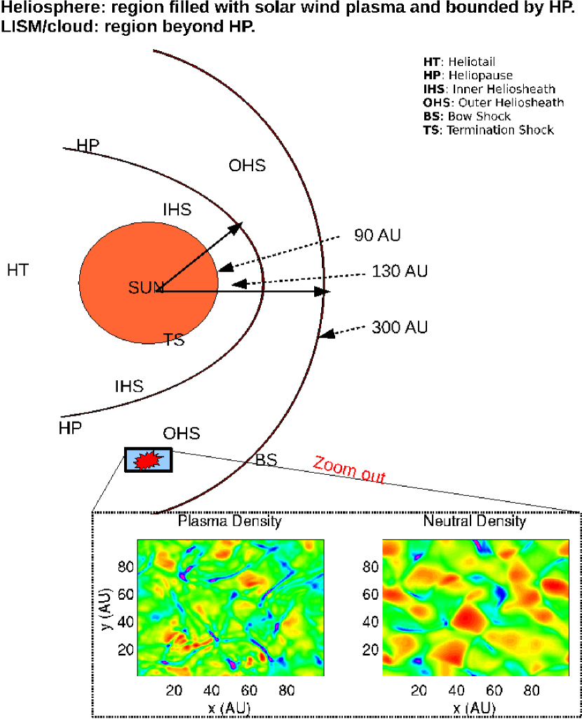
Figure 6: Schematic illustrating the plasma neutral simulation regions both in the local interstellar medium and in the outer heliosheath (see Zank (1999) for a review of the solar wind interaction with the local ISM).

In view of these comments, we have developed a self-consistent plasma-neutral ISM turbulence simulation model based on fluid modeling of neutral and plasma fluids (Zank, 1999; Pauls et. al, 1995; Zank et al., 1996). Our model treats the plasma and neutral species as distinguishable fluids and couples them through charge exchange. The model essentially employs a set of magnetohydrodynamic equations that describe the turbulent plasma motions, whereas the neutrals are described by hydrodynamic equations. A fluid approach for the local interstellar medium is justifiable since the charge exchange and collisional mean free path ensures approximate thermodynamical equipartition between plasma and neutral species with the result that both plasma and neutrals can be described by a Maxwellian distribution. Besides the local ISM, the outer heliosheath can also be described reasonably well by a fluid model of this kind, as was done in the model of Pauls et. al (1995). For a non-equilibrated description, a more elaborate multi-fluid model can be developed, as was done by Zank et al. (1996); Zank & Pauls (1996), and this could be applied to straightforwardly to both the outer heliosheath and very local ISM. This would be more important to the outer heliosheath since a multi-fluid model would then include hot inner heliosheath neutral atoms deposited through secondary charge exchange in the outer heliosheath (Zank et al., 1996; Zank & Pauls, 1996; Zank, 1999). The schematic in Fig. (6) depicts the simulation regions in which we are particularly interested i.e. the outer heliosheath and the local interstellar medium. The importance of ISM turbulence is clearly evident from this figure in the context of cosmic ray modulation, large-scale heliospheric structure and particle acceleration.

In this paper, we focus on the multi-scale evolution of a partially ionized plasma, comprising multiple fluids, where each fluid evolves under the influence of the other through a complex interaction process. We investigate the energy cascade between LISM turbulent-fluctuations in a partially ionized plasma where the plasma and neutral gas are coupled through charge exchange. Here, we, present a numerical simulation of ISM turbulence that self-consistently evolves both the plasma and neutral fluids when coupled by charge exchange. We restrict our attention to a neutral hydrogen (H) gas, so that plasma and neutral densities are conserved by charge exchange interactions. Hence the corresponding continuity equations do not include charge exchange terms. One of the points that emerges from our coupled multi fluid LISM simulations is that neutrals enhance turbulent cascade rates and lead to much steeper spectra compared to that predicted by the usual Kolmogorov theory (Kolmogorov, 1941) for pure MHD or hydrodynamics (Shaikh & Zank, 2007). In Section 2, we discuss the equations of a coupled plasma-neutral ISM turbulence model, their validity, the underlying assumptions and the normalizations. Section 3 deals with a quantitative derivation of charge exchange source terms, associated with the plasma and neutral fluids, based on the time-dependent Boltzmann equation. Section 4 describes the results of our nonlinear, coupled, self-consistent ISM fluid simulations. It is shown, in section 5, that the coupling of plasma and neutral fluids leads to an enhanced spectral transfer in the inertial range, which results in a steeper ISM turbulent spectrum than predicted by the Kolmogorov theory. Finally, conclusions are presented in Section 6.

2 Model Equations for a partially ionized LISM

The assumptions that are intrinsic to our model of turbulence in a partially ionized ISM are the following. (i) Fluctuations in the plasma and neutral fluids are isotropic, homogeneous, thermally equilibrated and turbulent, and (ii) Neither a mean magnetic field nor velocity flows are present initially. Local mean flows may subsequently be generated by self-consistently excited nonlinear instabilities. (iii) The characteristic turbulent correlation length-scales ($\lambda_{c}\sim 1/k_{c}$) are typically bigger than charge-exchange mean free path lengths ($\lambda_{ce}\sim 1/k_{ce}$) in the ISM flows, i.e $\lambda_{c}\gg\lambda_{ce}$ or $k_{ce}/k_{c}\gg 1$. The latter inequality is also consistent with Florinski et al (2003, 2005). Nevertheless, they are large enough to treat any localized shocks as smooth discontinuities. In other words, the characteristic shock length-scales are small compared to the ISM turbulent fluctuation length-scales, and finally (iv) boundary conditions are periodic, essentially a box of interstellar plasma, which is a natural and most appropriate choice for modeling turbulence in the local ISM.

While most of the above assumptions are appropriate to realistic ISM turbulent flows, so allowing us to use MHD and hydrodynamic descriptions for the plasma and the neutral components respectively, the latter has been criticized in the context of heliospheric flows within the heliopause owing to the large charge-exchange mean free path (about the size or even bigger than the extent of the heliosphere). The use of a fluid description for neutrals in the inner heliosheath is therefore inappropriate. In the LISM and outer heliosheath, we are nonetheless not restricted by a large mfp because the plasma and neutral fluid remain close to thermal equilibirium and behave as Maxwellian fluids. Our model simulates the local ISM and outer heliosheath. The fluid model describing nonlinear turbulent processes in the interstellar medium, in the presence of charge exchange, can be cast into plasma density ($\rho_{p}$), velocity (${\bf U}_{p}$), magnetic field (${\bf B}$), pressure ($P_{p}$) components according to the conservative form

$$\frac{\partial{\bf F}_{p}}{\partial t}+\nabla\cdot{\bf Q}_{p}={\cal Q}_{p,n},$$ (1)

where,

$${\bf F}_{p}=\left[\begin{array}[]{c}\rho_{p}\\ \rho_{p}{\bf U}_{p}\\ {\bf B}\\ e_{p}\end{array}\right],{\bf Q}_{p}=\left[\begin{array}[]{c}\rho_{p}{\bf U}_{p}\\ \rho_{p}{\bf U}_{p}{\bf U}_{p}+\frac{P_{p}}{\gamma-1}+\frac{B^{2}}{8\pi}-{\bf B}{\bf B}\\ {\bf U}_{p}{\bf B}-{\bf B}{\bf U}_{p}\\ e_{p}{\bf U}_{p}-{\bf B}({\bf U}_{p}\cdot{\bf B})\end{array}\right],\\ {\cal Q}_{p,n}=\left[\begin{array}[]{c}0\\ {\bf Q}_{M}({\bf U}_{p},{\bf V}_{n},\rho_{p},\rho_{n},T_{n},T_{p})\\ 0\\ Q_{E}({\bf U}_{p},{\bf V}_{n},\rho_{p},\rho_{n},T_{n},T_{p})\end{array}\right]$$

and

$$e_{p}=\frac{1}{2}\rho_{p}U_{p}^{2}+\frac{P_{p}}{\gamma-1}+\frac{B^{2}}{8\pi}.$$

The above set of plasma equations is supplemented by $\nabla\cdot{\bf B}=0$ and is coupled self-consistently to the ISM neutral density ($\rho_{n}$), velocity (${\bf V}_{n}$) and pressure ($P_{n}$) through a set of hydrodynamic fluid equations,

$$\frac{\partial{\bf F}_{n}}{\partial t}+\nabla\cdot{\bf Q}_{n}={\cal Q}_{n,p},$$ (2)

where,

$${\bf F}_{n}=\left[\begin{array}[]{c}\rho_{n}\\ \rho_{n}{\bf V}_{n}\\ e_{n}\end{array}\right],{\bf Q}_{n}=\left[\begin{array}[]{c}\rho_{n}{\bf V}_{n}\\ \rho_{n}{\bf V}_{n}{\bf V}_{n}+\frac{P_{n}}{\gamma-1}\\ e_{n}{\bf V}_{n}\end{array}\right],\\ {\cal Q}_{n,p}=\left[\begin{array}[]{c}0\\ {\bf Q}_{M}({\bf V}_{n},{\bf U}_{p},\rho_{p},\rho_{n},T_{n},T_{p})\\ Q_{E}({\bf V}_{n},{\bf U}_{p},\rho_{p},\rho_{n},T_{n},T_{p})\end{array}\right],$$

$$e_{n}=\frac{1}{2}\rho_{n}V_{n}^{2}+\frac{P_{n}}{\gamma-1}.$$

Equations (1) to (2) form an entirely self-consistent description of the coupled ISM plasma-neutral turbulent fluid. Several points are worth noting. The charge-exchange momentum sources in the plasma and the neutral fluids, i.e. Eqs. (1) and (2), are described respectively by terms ${\bf Q}_{M}({\bf U}_{p},{\bf V}_{n},\rho_{p},\rho_{n},T_{n},T_{p})$ and ${\bf Q}_{M}({\bf V}_{n},{\bf U}_{p},\rho_{p},\rho_{n},T_{n},T_{p})$. A swapping of the plasma and the neutral fluid velocities in this representation corresponds, for instance, to momentum changes (i.e. gain or loss) in the plasma fluid as a result of charge exchange with the ISM neutral atoms (i.e. ${\bf Q}_{M}({\bf U}_{p},{\bf V}_{n},\rho_{p},\rho_{n},T_{n},T_{p})$ in Eq. (1)). Similarly, momentum change in the neutral fluid by virtue of charge exchange with the plasma ions is indicated by ${\bf Q}_{M}({\bf V}_{n},{\bf U}_{p},\rho_{p},\rho_{n},T_{n},T_{p})$ in Eq. (2). In the absence of charge exchange interactions, the plasma and the neutral fluid are de-coupled trivially and behave as ideal fluids. While the charge-exchange interactions modify the momentum and the energy of plasma and the neutral fluids, they conserve density in both the fluids (since we neglect photoionization and recombination). Nonetheless, the volume integrated energy and the density of the entire coupled system will remain conserved in a statistical manner. The conservation processes can however be altered dramatically in the presence of any external forces. These can include large-scale random driving of turbulence due to any external forces or instabilities, supernova explosions, stellar winds, etc. Finally, the magnetic field evolution is governed by the usual induction equation, i.e. Eq. (1), that obeys the frozen-in-field theorem unless some nonlinear dissipative mechanism introduces small-scale damping.

The underlying ISM turbulence model can be non-dimensionalized straightforwardly using a typical ISM scale-length ($\ell_{0}$), density ($\rho_{0}$) and velocity ($v_{0}$). The normalized plasma density, velocity, energy and the magnetic field are respectively; $\bar{\rho}_{p}=\rho_{p}/\rho_{0},\bar{\bf U}_{p}={\bf U}_{p}/v_{0},\bar{P}_{p}=P_{p}/\rho_{0}v_{0}^{2},\bar{\bf B}={\bf B}/v_{0}\sqrt{\rho_{0}}$. The corresponding neutral fluid quantities are $\bar{\rho}_{n}=\rho_{n}/\rho_{0},\bar{\bf U}_{n}={\bf U}_{n}/v_{0},\bar{P}_{n}=P_{n}/\rho_{0}v_{0}^{2}$. The momentum and the energy charge-exchange terms, in the normalized form, are respectively $\bar{\bf Q}_{m}={\bf Q}_{m}\ell_{0}/\rho_{0}v_{0}^{2},\bar{Q}_{e}=Q_{e}\ell_{0}/\rho_{0}v_{0}^{3}$. The non-dimensional temporal and spatial length-scales are $\bar{t}=tv_{0}/\ell_{0},\bar{\bf x}={\bf x}/\ell_{0}$. Note that we have removed bars from the set of normalized coupled ISM model equations (1) & (2). The charge-exchange cross-section parameter ($\sigma$), which does not appear directly in the above set of equations (see the subsequent section for more detail), is normalized as $\bar{\sigma}=n_{0}\ell_{0}\sigma$, where the factor $n_{0}\ell_{0}$ has dimension of (area)^-1. By defining $n_{0},\ell_{0}$ through $\sigma_{ce}=1/n_{0}\ell_{0}=k_{ce}^{-2}$, we see that there exists a critical charge exchange wavenumber ($k_{ce}$) associated with the coupled ISM plasma-neutral turbulent system. For a characteristic density, this corresponds physically to an area defined by the charge exchange mode being equal to (mfp)². Thus the larger the area, the higher is the probability of charge exchange between plasma ions and neutral atoms, as illustrated in Fig. (2). To be precise, ‘$k_{ce}$’ is a (lengthscale)^-1 that typically helps us determine whether or not a particular turbulent fluctuation length scale undergoes charge exchange in our model. It is strictly in that sense, we refer to it as a critical wavenumber. Clearly, there exist three different regimes depending on whether (i) $k<k_{ce}$, (ii) $k\simeq k_{ce}$ or (iii) $k>k_{ce}$. In the heliosheath, the probability that charge exchange can directly modify those modes satisfying $k<k_{ce}$ is high compared to modes satisfying $k>k_{ce}$. Since the charge exchange length-scales are much smaller than the ISM turbulent correlation scales, this further allows many charge exchange interactions amongst the nonlinear turbulent ISM modes before they cascade energy in one unit convective time. This is illustrated schematically in Fig. (2).

It is interesting to compare our model with other work. Of particular relevance is the classic work by Kulsrud and Pearce (1969) who investigated the interaction of galactic comic rays and Alfién waves in the interstellar medium and also considered ion-neutral collision as a damping mechanism for Alfvén waves. Ion-neutral collisions are also reported by McIvor (1977) to be a dominant mechanism for damping interstellar medium turbulence. The damping (due to ion-neutral collisions) rates for Alfvén waves estimated by Kulsrud and Pearce (1969) are based on $\nu_{0}\simeq n_{0}v_{th}\sigma$, where $\nu_{0},n_{0},v_{th}$ and $\sigma$ are respectively the ion-neutral collision frequency, neutral density, thermal speed and collision cross-section. The damping wavenumber associated with this frequency can be estimated to be $k\simeq n_{0}v_{th}\sigma/V_{A}$. The latter determines essentially the dissipation wavenumber associated with the damping of small scale Alfvén waves in ISM turbulence (Kulsrud and Pearce 1969). The turbulent cascade is further expected to be terminated beyond this wavenumber. It is clear from this expression that the higher the thermal speed, the larger the dissipation wavenumber. Correspondingly in real space, dissipation will be concentrated on smaller length-scales for higher thermal speeds. Furthermore, the thermal speed is also proportional to the temperature. Thus, given the heliosheath parameters, $v_{Thu}$ associated with heliosheath neutral atoms will be at least two orders of magnitude larger compared with that results from Eq. (47) in Kulsrud and Pearce (1969). This will correspond to a larger dissipative wavenumber in the heliosheath region and essentially means that charge exchange interactions are restricted to only those eddies whose length-scales are comparable to the dissipative length-scales of turbulence. It is not clear if this scenario holds in inner/outer heliosheath turbulence where charge exchange interactions, in principle, can modify any length scale in the inertial range. Part of the reason resides with the fact that charge exchange modifications are proportional to the relative speed between ion and neutral fluids and corresponding densities which can obviously alter the nonlinear cascades by influencing the combined momenta and energies of both the fluids in a self-consistent and subtle manner. Additionally, Kulsrud and Pearce (1969), as does McIvor (1977), assumed a fixed neutral density while computing the damping rates associated with Alfvén waves in ISM turbulence. While a fixed neutral density can modify the linear growth rates of the underlying waves, it does not itself evolve and hence no back reaction on Alfvén waves and vice versa can be expected. By contrast, our model self-consistently evolves neutral and plasma and describes the mutual feedback of one species on the other. This not only alters the linear interaction process, but it also influences the nonlinear coupling in a subtle manner not readily describable by means of any linear analytic theory. A self-consistent coupling is absolutely essential to understand nonlinear turbulent cascades in the inner/outer heliosheath. It is to be noted further that we do not attempt to investigate damping of heliosheath turbulence by Alfvén waves that experience ion-neutral collisions, unlike McIvor (1977). While Alfvén waves are intrinsically present in our model, turbulent cascades are least affected by them along the mean magnetic field (Shebalin & Montgomery 1983). Alfvén waves can be crucial in providing a local anisotropy in the spectral transfer due to a mean or local field though. However, our prime focus here is to develop an understanding of heliosheath turbulence where plasma and neutral fluids evolve through a mutual interaction mediated by charge exchange. As evident from the complexity associated with these interactions, nonlinear turbulent cascades are likely to be affected at any length scale in the heliosheath inertial range, unlike a linear dissipative processes.

In the subsequent section, we derive an exact quantitative form of the sources due to charge exchange in ISM turbulence.

3 Charge Exchange Sources

The charge exchange terms can be obtained from the Boltzmann transport equation that describes the evolution of a neutral distribution function $f_{n}=f({\bf x},v_{x},v_{y},v_{z},t)$ in a six-dimensional phase space defined respectively by position and velocity vectors $({\bf x},v_{x},v_{y},v_{z})$ at each time $t$. Here we follow Pauls et. al (1995) in computing the charge exchange terms from various moments of the Boltzmann equation. The Boltzmann equation for the neutral distribution contains a source term proportional to the proton distribution function $f_{p}$ and a loss term proportional to the neutral distribution function $f_{n}$,

$$\frac{\partial f_{n}}{\partial t}+{\bf v}_{n}\cdot\nabla f_{n}+\frac{\bf F}{m}\cdot\nabla_{{\bf v}_{n}}f_{n}=f_{p}({\bf x},v_{x},v_{y},v_{z},t)\int f_{n}({\bf x},v_{x},v_{y},v_{z},t)|{v}_{n}-{u}_{p}|\sigma_{\rm ex}(v_{rel})d^{3}{v}_{n}$$

$$-f_{n}({\bf x},v_{x},v_{y},v_{z},t)\int f_{p}({\bf x},v_{x},v_{y},v_{z},t)|{u}_{p}-{v}_{n}|\sigma_{\rm ex}(v_{rel})d^{3}{u}_{p}.$$ (3)

Here $f_{p},~{}{u}_{p}$ represent respectively the proton distribution function and velocity. $\sigma_{\rm ex}$ is the charge exchange cross-section (between neutrals and plasma protons), $m$ is the mass of particle, and ${\bf F}$ represents forces acting on the fluid. The charge exchange parameter has a logarithmically weak dependence on the relative speed ($v_{rel}=|{u}_{p}-{v}_{n}|$) of the neutrals and the protons through $\sigma_{\rm ex}=[(2.1-0.092\ln(v_{rel}))10^{-7}cm]^{2}$ (Fite et al, 1962). This cross-section is valid as long as energy does not exceed $1eV$, which usually is the case in the inner/outer heliosphere. Beyond $1eV$ energy, this cross-section yields a higher neutral density. This issue is not applicable to our model and hence we will not consider it here. The density, momentum, and energy of the thermally equilibrated Maxwellian proton and neutral fluids can be computed from Eq. (3) by using the zeroth, first and second moments $\int f_{\xi}d^{3}\xi,\int m{\bf\xi}f_{\xi}d^{3}\xi$ and $\int m\xi^{2}/2f_{\xi}d^{3}\xi$ respectively, where $\xi={u}_{p}$ or ${v}_{n}$. Since charge exchange conserves the density of the proton and neutral fluids, there are no sources in the corresponding continuity equations. We, therefore, need not compute the zeroth moment of the distribution function. Computing directly the first moment from Eq. (3), we obtain the neutral fluid momentum equation as given by Eq. (2). The entire rhs of Eq. (3) can now be replaced by a momentum transfer function ${\bf Q}_{M}({v}_{n},{u}_{p})$ which reads

$${\bf Q}_{M}({v}_{n},{u}_{p})=\bar{\mu}({u}_{p},{v}_{n})-\bar{\mu}({v}_{n},{u}_{p}),$$ (4)

where ${\bf Q}_{M}$ and $\bar{\mu}$, the transfer integral, are vector quantities. The transfer integrals describe the charge exchange transfer of momentum from proton to neutral fluid and vice versa. The first term on the rhs of Eq. (4) can be expressed by

$$\bar{\mu}({u}_{p},{v}_{n})=f_{p}({\bf x},v_{x},v_{y},v_{z},t)\beta({u}_{p},{v}_{n})$$

where,

$$\beta({u}_{p},{v}_{n})=\int f_{n}({\bf x},v_{x},v_{y},v_{z},t)|{v}_{n}-{u}_{p}|\sigma_{\rm ex}(v_{rel})d^{3}{v}_{n}.$$

Considering a Maxwellian distribution for the neutral atoms, we simplify $\beta({u}_{p},{v}_{n})$ as follows,

$$\beta({u}_{p},{v}_{n})=\sigma_{\rm ex}n_{n}V_{T_{n}}\sqrt{\frac{4}{\pi}+\frac{({v}_{n}-{u}_{p})^{2}}{V_{T_{n}}^{2}}}.$$

Note that the above expression emerges directly from a straightforward integration of sources in the rhs of the Boltzmann Eq. (3). To obtain the expression for the momentum transferred from proton to neutral (or vice versa), we need to take a second moment of the $\bar{\mu}({u}_{p},{v}_{n})$ expression. This is shown in the following,

$$\bar{\mu}({u}_{p},{v}_{n})=m{\bf v}_{n}I_{0}({u}_{p},{v}_{n})+m({\bf u}_{p}-{\bf v}_{n})I_{1}({u}_{p},{v}_{n}).$$

where $I_{0}$ and $I_{1}$ are transfer integrals that can be written as follows,

$$I_{0}({u}_{p},{v}_{n})=\int f_{p}({\bf x},v_{x},v_{y},v_{z},t)\beta({u}_{p},{v}_{n})~{}d^{3}{u}_{p};$$

$$I_{1}({u}_{p},{v}_{n})=\int{v}_{n}f_{p}({\bf x},v_{x},v_{y},v_{z},t)\beta({u}_{p},{v}_{n})~{}d^{3}{u}_{p}.$$

Assuming a Maxwellian distribution for plasma protons and using $\beta({u}_{p},{v}_{n})$ from the above expression, we can straightforwardly evaluate the transfer integrals $I_{0}$ and $I_{1}$ (see Pauls et al (1995) for details). We further write the complete form of the first term on the rhs of Eq. (4) as follows,

$$\bar{\mu}({u}_{p},{v}_{n})=m\sigma_{\rm ex}n_{p}n_{n}\left[U_{{u}_{p},{v}_{n}}^{\ast}{\bf v}_{n}-({\bf u}_{p}-{\bf v}_{n})\frac{V_{T_{n}}^{2}}{\delta V_{{u}_{p},{v}_{n}}}\right].$$

In a similar manner, we can evaluate the second term on the rhs of Eq. (4), which yields the following form,

$$\bar{\mu}({v}_{n},{u}_{p})=m\sigma_{\rm ex}n_{p}n_{n}\left[U_{{v}_{n},{u}_{p}}^{\ast}{\bf u}_{p}-({\bf v}_{n}-{\bf u}_{p})\frac{V_{T_{p}}^{2}}{\delta V_{{v}_{n},{u}_{p}}}\right],$$

where $\delta V_{{u}_{p},{v}_{n}}=\left[4\left(\frac{4}{\pi}V_{T_{p}}^{2}+\Delta U^{2}\right)+\frac{9\pi}{4}V_{T_{n}}^{2}\right]^{1/2},\delta V_{{v}_{n},{u}_{p}}=\left[4\left(\frac{4}{\pi}V_{T_{n}}^{2}+\Delta U^{2}\right)+\frac{9\pi}{4}V_{T_{n}}^{2}\right]^{1/2}$ and $U^{\ast}=U_{{u}_{p},{v}_{n}}^{\ast}=U_{{v}_{n},{u}_{p}}^{\ast}=\left[\frac{4}{\pi}V_{T_{p}}^{2}+\frac{4}{\pi}V_{T_{n}}^{2}+\Delta U^{2}\right]^{1/2},\Delta{u}={u}_{p}-{v}_{n}$ (Pauls et. al, 1995). On substituting these expressions in the momentum transfer function, we obtain

$${\bf Q}_{M}({v}_{n},{u}_{p})=m\sigma_{\rm ex}n_{p}n_{n}({\bf v}_{n}-{\bf u}_{p})\left[U^{\ast}+\frac{V_{T_{n}}^{2}}{\delta V_{{u}_{p},{v}_{n}}}-\frac{V_{T_{p}}^{2}}{\delta V_{{v}_{n},{u}_{p}}}\right].$$ (5)

Equation (5) together with Eq. (2) yields the momentum equation for the neutral gas. Swapping the plasma and neutral fluid velocities yields the corresponding source term for the proton fluid momentum equation. The gain or the loss in neutral or proton fluid momentum depends upon the charge exchange sources, which depend upon the relative speeds between neutrals and the protons. The thermal speeds of proton and neutral gas in Eq. (5) are given respectively by $V_{T_{p}}^{2}=2K_{B}T_{p}/m$ (the factor 2 arises because of thermal equilibration in that it is assumed that the temperature of the plasma electrons and protons are nearly identical so that $T_{p}=T_{e}+T_{\rm proton}\simeq 2T_{p}$) and $V_{T_{n}}^{2}=K_{B}T_{n}/m$. The corresponding temperatures are related to the pressures by $P_{p}=2n_{p}K_{B}T_{p}$ and $P_{n}=n_{n}K_{B}T_{n}$, where $n_{n},T_{n},n_{p},T_{p}$ are respectively the neutral and plasma density and the temperature, and $K_{B}$ is the Boltzmann constant.

The moment, $\int m\xi^{2}/2f_{\xi}d^{3}\xi$, of the Boltzmann Eq. (3) yields an energy equation for the neutral fluid whose rhs contains the charge exchange energy transfer function

$$Q_{E}({v}_{n},{u}_{p})=\eta({u}_{p},{v}_{n})-\eta({v}_{n},{u}_{p}),$$

where $\eta({u}_{p},{v}_{n}),~{}\eta({v}_{n},{u}_{p})$ are the energy transfer (from neutral to proton and vice versa) rates. These functions can be computed as follows:

$$\eta({u}_{p},{v}_{n})=\frac{1}{2}mV_{n}^{2}\sigma_{\rm ex}n_{p}n_{n}U^{\ast}+\frac{3}{4}mV_{T_{n}}^{2}\sigma_{\rm ex}n_{p}n_{n}\Delta V_{{u}_{p},{v}_{n}}-m\sigma_{\rm ex}n_{p}n_{n}{\bf v}_{n}\cdot({\bf u}_{p}-{\bf v}_{n})\frac{V_{T_{n}}^{2}}{\delta V_{{u}_{p},{v}_{n}}}$$

and

$$\eta({v}_{n},{u}_{p})=\frac{1}{2}mV_{n}^{2}\sigma n_{p}n_{n}U^{\ast}+\frac{3}{4}mV_{T_{p}}^{2}\sigma_{\rm ex}n_{p}n_{n}\Delta V_{{v}_{n},{u}_{p}}-m\sigma_{\rm ex}n_{p}n_{n}{\bf u}_{p}\cdot({\bf v}_{n}-{\bf u}_{p})\frac{V_{T_{p}^{2}}}{\delta V_{{v}_{n},{u}_{p}}}.$$

The total energy transfer from neutral to proton fluid, due to charge exchange, can then be written as,

$$Q_{E}({v}_{n},{u}_{p})=\frac{1}{2}m\sigma_{\rm ex}n_{p}n_{n}U^{\ast}(V_{n}^{2}-U_{p}^{2})+\frac{3}{4}m\sigma_{\rm ex}n_{p}n_{n}(V_{T_{n}}^{2}\Delta V_{{u}_{p},{v}_{n}}-V_{T_{p}}^{2}\Delta V_{{v}_{n},{u}_{p}})$$

$$-m\sigma_{\rm ex}n_{p}n_{n}\left[{\bf v}_{n}\cdot({\bf u}_{p}-{\bf v}_{n})\frac{V_{T_{n}}^{2}}{\delta V_{{u}_{p},{v}_{n}}}-{\bf u}_{p}\cdot({\bf v}_{n}-{\bf u}_{p})\frac{V_{T_{p}^{2}}}{\delta V_{{v}_{n},{u}_{p}}}\right],$$ (6)

with $\Delta V_{{u}_{p},{v}_{n}}=[\frac{4}{\pi}V_{T_{p}}^{2}+\frac{64}{9\pi}V_{T_{n}}^{2}+\Delta U^{2}]^{1/2}~{}{\rm and}~{}\Delta V_{{v}_{n},{u}_{p}}=[\frac{4}{\pi}V_{T_{n}}^{2}+\frac{64}{9\pi}V_{T_{p}}^{2}+\Delta U^{2}]^{1/2}$. A similar expression for the energy transfer charge exchange source term of plasma energy in Eq. (1) can be obtained by exchanging the plasma and neutral fluid velocities. In the normalized momentum and energy charge exchange source terms, the factor $m\sigma_{\rm ex}$ in Eqs. (5) & (3) is simply replaced by $\bar{\sigma}$.

4 Nonlinear Simulation of Energy Cascades

It is clear from previous sections that the interaction of the neutrals with a plasma introduces characteristic length and time scales that can separate characteristic time and length scales in ISM turbulence. For instance, the plasma-neutral fluid coupling in the ISM fluctuations introduces charge exchange modes, $k_{ce}$, that are distinctively different from the characteristic turbulent mode $k$. Typically, characteristic turbulent length-scales ($\lambda_{c}\sim 1/k$) are much bigger than the charge exchange length-scales $\lambda_{ce}\sim 1/k_{ce}$, since for example, $\lambda_{c}\sim(100-1000)\lambda_{ce}$ in the ISM cloud (Florinski et al, 2003, 2005). This essentially corresponds to $k_{ce}/k\gg 1$ (Zank, 1999; Florinski et al, 2003, 2005). It should be noted that the charge exchange sources in the neutral and the plasma fluids do not merely damp the smallest scale fluctuations, such as is the case with linear collisional dissipation in turbulent fluid flows, but they can alter the nonlinear cascade rate dramatically (Shaikh et al, 2006; Shaikh & Zank, 2007). Because of its complex nonlinear character (see Eqs. (5) & (3)), charge exchange can be effective on a variety of turbulent length-scales unlike linear dissipation which is operative on small length-scales only. The effect and influence of the charge exchange source terms on the turbulent inertial range of coupled neutral and plasma fluids is therefore a subtle issue and is not restricted only to the damping of small scales in partially ionized, magnetized ISM turbulence. With this in mind, we carry out two different sets of simulations of Eqs. (1) & (2), to discern the effects of charge exchange on the ISM plasma-neutral system. In the first set of simulations, Eqs. (1) & (2) are decoupled (i.e. no charge exchange coupling is assumed) and each evolves as an ideal fluid, whereas in the second set the coupling is included self-consistently. The former provides a reference simulation against which to investigate the coupled system.

A two-dimensional (2D) nonlinear fluid code was developed to numerically integrate Eqs. (1) to (2). The 2D simulations are not only computationally less expensive (compared to a fully 3D calculation), but they offer significantly higher resolution (to compute inertial range turbulence spectra) even on moderately-sized clusters like our local Beowulf. The spatial discretization in our code uses a discrete Fourier representation of turbulent fluctuations based on a pseudospectral method, while we use a Runge Kutta 4 method for the temporal integration. All the fluctuations are initialized isotropically (no mean fields are assumed) with random phases and amplitudes in Fourier space. This algorithm ensures conservation of total energy and mean fluid density per unit time in the absence of charge exchange and external random forcing. Additionally, $\nabla\cdot{\bf B}=0$ is satisfied at each time step. Our code is massively parallelized using Message Passing Interface (MPI) libraries to facilitate higher resolution. The initial isotropic turbulent spectrum of fluctuations is chosen to be close to $k^{-2}$ with random phases in both $x$ and $y$ directions. The choice of such (or even a flatter than -2) spectrum does not influence the dynamical evolution as the final state in our simulations progresses towards fully developed turbulence. While the ISM turbulence code is evolved with time steps resolved self-consistently by the coupled fluid motions, the nonlinear interaction time scales associated with the plasma $1/{\bf k}\cdot{\bf U}_{p}({\bf k})$ and the neutral $1/{\bf k}\cdot{\bf V}_{n}({\bf k})$ fluids can obviously be disparate. Accordingly, turbulent transport of energy in the plasma and the neutral ISM fluids takes place on distinctively separate time scales.

Because of the different nonlinear time scales associated with the plasma and neutral fluids, mode structures can be different in the two fluids when they are evolved together and in isolation (i.e. decoupled). The former is shown in

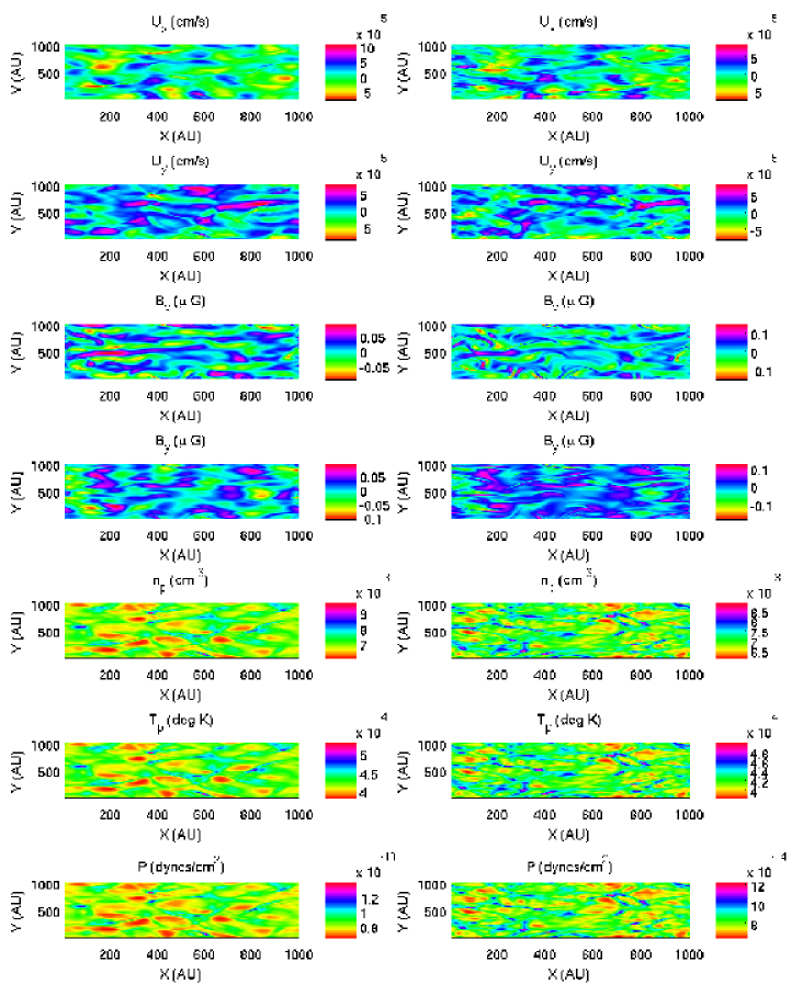
Figure 1: .

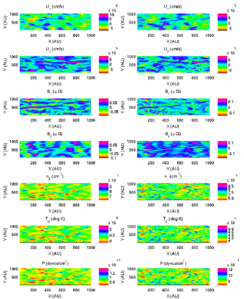
Figure 8: (Left column) Mode structures of plasma when coupled with the neutral ISM fluid. The local ISM case is considered where typical LISM parameters are; $\gamma=5/3,n_{0_{plasma}}=0.06cm^{-3},n_{0_{neutral}}=0.18cm^{-3},T=6500K,V_{th}=10km/s,\sigma=6.9\times 10^{-15},l_{0}=200AU,L({\rm boxlength})=5l_{0}$. (Right column) The corresponding quantities for an uncoupled ISM plasma simulation measured at a similar time step (i.e. $t=20$ in normalized units). Notice the magnetic field structures in the uncoupled case showing the formation of thin (or sheet-like) structures unlike the coupled system. Also notice the differences in the density fields.

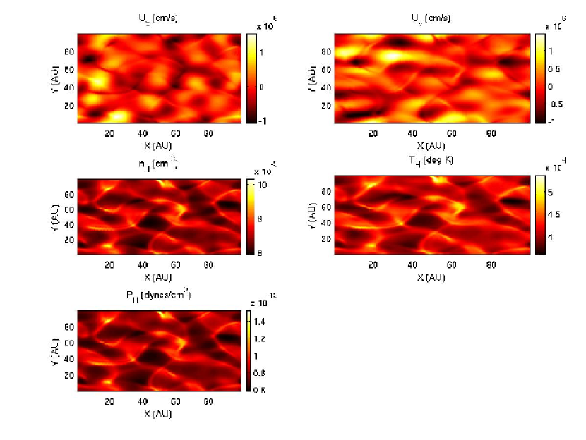
Figure 9: The corresponding mode structures of neutral fluid in the presence of a plasma fluid. Simulation parameters are described in the previous figure.

The figures respectively show the evolution of various physical quantities in the plasma-neutral coupled system for a typical set of ISM parameters as described in the captions (for typical ISM parameters, see also Zank (1999); Zank et al. (1996); Heerikhuisen et al (2006); Florinski et al (2003, 2005)). In the absence of charge exchange (see Fig. (8), right column), the plasma fluid evolves as an ideal MHD fluid and is known to typically develop sheet-like structures in the magnetic field (Biskamp, 2003). By contrast, the evolution of the magnetic field is modified substantially when the two fluids are coupled through charge exchange. For instance, the sheet-like structures present in the turbulent magnetic field of the uncoupled plasma system instead are smeared in the coupled plasma-neutral system on the typical sheet-formation time-scales of ideal MHD. The neutral fluid, under the action of charge exchange terms, tends to modify the cascade rates by isotropizing the ISM turbulence on a slower time scale. This point is further elucidated in the subsequent section based on Kolmogorov-like phenomenological arguments. However if the coupled system is evolved further, sheets do form eventually in the magnetic field (after a relatively long time compared to the ideal MHD time-scales) and a turbulent equipartition is set up in the plasma and the neutral fluid modes. In any event, the small-scale sheet-like structures in magnetic field compress (or pinch) the plasma density. Hence the density fluctuations develop identical (thinner than) sheet-like structures that co-exist with small-scale turbulent fluctuations in their spectrum as shown in Fig. (8). The neutral fluid, on the other hand, evolves isotropically as stated above by forming relatively large-scale structures (see Fig. (9)).

5 Energy Spectra

Spectral transfer in ISM turbulence progresses under the action of nonlinear interactions as well as charge exchange sources. Energy cascades amongst turbulent eddies of various scale sizes and between the plasma and the neutral fluids. In a freely decaying case, plasma and neutral fluids evolve under the influence of charge exchange forces which dramatically affect the energy cascades in the inertial range. This is evident from

Figure 2: w

here Kolmogorov-like fully developed turbulent spectra in the inertial range are shown respectively for the coupled neutral and plasma fluids. The neutral fluid energy spectrum in the inertial regime for the coupled system exhibits a $k^{-\alpha}$ spectrum, where the spectral index $\alpha\approx 3.2$. On the other hand, the spectral index for plasma magnetic and kinetic energy spectra for the coupled system is $\alpha\approx 2.4$. The inertial range spectral indices for the coupled plasma-neutral system in our simulations show a significant deviation from their corresponding uncoupled analogues which are respectively $-3$ and $-1.7$ for the neutral and plasma fluids, also plotted in

Figure 3: .

The inertial range turbulent spectra are much steeper for the coupled ISM plasma-neutral system than the corresponding uncoupled or isolated neutral and plasma fluids in the decaying turbulence regime. Consequently, the steep turbulent spectra in the coupled ISM plasma-neutral system gives rise to an enhanced spectral transfer amongst the inertial range modes, and the energy cascade rates associated with the plasma and neutral (coupled) fluids can be understood by invoking a Kolmogorov-like phenomenology as described in the following.

The typical nonlinear interaction time-scale in ordinary (i.e. uncoupled) plasma and/or neutral turbulence is given by

$$\tau_{nl}\sim\frac{\ell_{0}}{v_{\ell}}\sim(kv_{k})^{-1},$$ (7)

where $v_{k}$ or $v_{\ell}$ is the velocity of turbulent eddies. In the presence of charge exchange interactions, the ordinary nonlinear interaction time-scale of fluid turbulence is modified by a factor $k_{ce}/k$ such that the new nonlinear interaction time-scale of ISM turbulence is now

$$\tau_{NL}\sim\frac{k_{ce}}{k}\frac{1}{kv_{k}}.$$ (8)

The main justification of using the above expression originates from the fact that turbulent cascade is determined typically by the nonlinear interaction time ($\tau_{nl}\sim 1/kv_{k}$, where $\tau_{nl}$ is the eddy interaction time, $k$ is characteristic turbulent wavenumber, and $v_{k}$ is characteristic speed of eddy in wavenumber space) associated with the convection of turbulent eddies in the fluid momentum equation. Note that this time scale follows from Kolmogorov’s phenomenology (Kolmogorov 1941) and corresponds essentially to the eddy interaction time in an ideal, non interacting, and non magnetized hydrodynamic-like turbulent fluid. Such time scales are essential to estimate spectral energy transfer (or cascades) rates ($\varepsilon\simeq E(k)/\tau_{nl}$, where $E(k)$ is turbulent energy per unit mode) in a hydrodynamic turbulent fluid. For a non-ideal, interacting and magnetized fluid, incorporating complex interactions amongst the turbulent eddies with a background or local mean magnetic field, the nonlinear eddy interaction time needs to be modified. This was first pointed out by Kraichnan (1965) in the context of magnetohydrodynamic (MHD) fluids where the interaction of turbulent eddies with Alfvén waves, excited as a result of a mean magnetic field, was addressed. Owing to the presence of waves in a MHD fluid, turbulent correlations between velocity and magnetic field and the corresponding energy transfer time are determined primarily by $\tau\sim(b_{0}k)^{-1}$, where $b_{0}$ is a typical amplitude of a local magnetic field and is dimensionally identical to that of the velocity field by virtue of Els$\ddot{\rm a}$sser’s symmetry (Kraichnan 1965). Note carefully the modification in the energy transfer (or cascade) time scale because of the wave-turbulent eddy interaction process. Since the convective time is the only nonlinear time scale involved in the spectral transfer of turbulent energy, it it this time that accounts entirely for the nonlinear cascade in the coupled plasma-neutral heliosheath turbulence. Likewise, we introduce an analogous modification in the coupled plasma-neutral ISM turbulence where the energy cascade time scale due to charge exchange interactions amongst turbulent eddies, is determined explicitly by the factor $k_{ce}/k$ (where the symbols have their usual meanings). It is this factor that determines how plasma and neutral fluids are coupled in heliosheath turbulence. Accordingly, the nonlinear spectral transfer time or the energy cascade rate is modified and is proportional to the factor $k_{ce}/k$ such that the new nonlinear eddy interaction time in the coupled plasma-neutral heliosheath turbulence is $\tau_{NL}\sim(k_{ce}/k)(1/kv_{k})$. The interaction time $\tau_{NL}$ obtained in this manner for our coupled plasma-neutral problem not only adequately reproduces all three different regimes of interactions, but it also consistently describes the underlying physics in the context of heliosheath turbulence.

On using the fact that $k_{ce}$ is typically larger than $k$ (or $k_{c}$, the characteristic turbulent mode, as defined elsewhere in the paper), i.e. $k_{ce}/k>1$ in the ISM (Florinski et al, 2003, 2005; Zank, 1999), the new nonlinear time is $k_{ce}/k$ times bigger than the old nonlinear time i.e. $\tau_{NL}\sim(k_{ce}/k)\tau_{nl}$. This enhanced nonlinear interaction time in ISM turbulence is likely to prolong turbulent energy cascade rates. It is because of this enhanced or prolonged interaction time that a relatively large spectral transfer of turbulent modes tends to steepen the inertial range turbulent spectra in both plasma and neutral fluids. By extending the above phenomenological analysis, one can deduce exact (analytic) spectral indices of the inertial range decaying turbulent spectra, as follows. The new nonlinear interaction time-scale of ISM turbulence can be rearranged as

$$\tau_{NL}\sim\frac{k_{ce}v_{k}}{kv_{k}}\frac{1}{kv_{k}}\sim\frac{\tau_{nl}^{2}}{\tau_{ce}},$$ (9)

where $\tau_{ce}\sim(k_{ce}v_{k})^{-1}$ represents the charge exchange time scale. The energy dissipation rate associated with the coupled ISM plasma-neutral system can be determined from $\varepsilon\sim E_{k}/\tau_{NL}$, which leads to

$$\varepsilon\sim\frac{v_{k}^{2}}{k_{ce}/k^{2}v_{k}}\sim\frac{k^{2}v_{k}^{3}}{k_{ce}}.$$ (10)

According to the Kolmogorov theory, the spectral cascades are local in $k$-space and the inertial range energy spectrum depends upon the energy dissipation rates and the characteristic turbulent modes, such that $E_{k}\sim\varepsilon^{\gamma}k^{\beta}$. Upon substitution of the above quantities and equating the power of identical bases, one obtains

$$E_{k}\sim\varepsilon^{2/3}k^{-7/3}$$ (11)

for the plasma spectrum (the forward cascade inertial range). The spectral index associated with this spectrum, i.e. $7/3\approx 2.33$, is consistent with the plasma spectrum observed in the (coupled ISM plasma-neutral) simulations (see

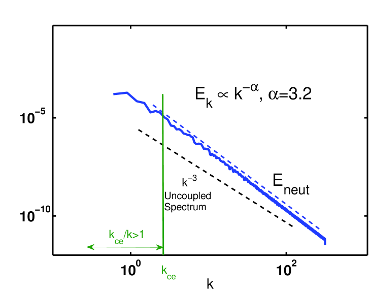
Figure 4: )

. Similar arguments in the context of neutral fluids, when coupled with the plasma fluid in ISM, lead to the energy dissipation rates

$$\varepsilon\sim\frac{k^{2}v_{k}^{2}}{k_{ce}/k^{2}v_{k}}.$$ (12)

This further yields the forward cascade (neutral) energy spectrum

$$E_{k}\sim\varepsilon^{2/3}k^{-11/3}$$ (13)

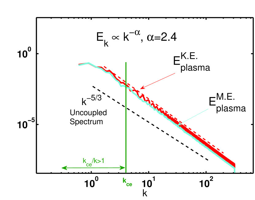
Figure 11: A similar steepening of turbulent spectra occurs in the plasma fluid when coupled to the neutrals through charge exchange. An uncoupled magnetofluid plasma exhibits a Kolmogorov-like $k^{-5/3}$ spectrum in the forward cascade regime (drawn schematically).

which is close to the simulation result shown in Fig. (11).

A key issue finally is to understand what role charge exchange modes play in coupled plasma-neutral ISM turbulence as they result essentially from the nonlinear charge exchange interactions. To address this issue, we plot charge exchange sources associated with the momentum and energy equations, Eqs. (1) & (2), in Fig. (12). It appears from Fig. (12) that spectral energy is transferred predominantly at the larger scales by means of charge exchange mode coupling processes. The latter couples the large-scales, or smaller than $k_{ce}$ modes, efficiently to low-$k$ ISM turbulent modes. It is primarily because of this $k_{ce}-k$ mode-coupling in the smaller $k$ part of the spectrum of the coupled plasma-neutral ISM turbulence, that energy is pumped efficiently at the lower $k$ inertial range turbulent modes. The efficient coupling of the Fourier modes at low $k$’s further enhances the nonlinear eddy time-scales associated with the coupled plasma-neutral turbulence system which is consistent with the scaling $\tau_{NL}\sim(k_{ce}/k)\tau_{nl}$, where $k_{ce}/k>1$, as described above. This consequently leads to the steepening of the inertial range spectra observed in

Figure 5: .

By contrast, higher $k$ modes, far from the energy cascade inertial range, are notably inefficient in transferring energy and momentum via charge exchange mode coupling interactions and are damped by small-scale dissipative processes in the coupled plasma-neutral ISM turbulence.

6 Conclusions

In conclusion, we have developed a self-consistent fluid model to describe nonlinear turbulent processes in a partially ionized and magnetized ISM gas. The charge exchange interactions couple the ISM plasma and the neutral fluids by exciting a characteristic charge exchange coupling mode $k_{ce}$, which is different from the characteristic turbulent mode $k$ of the coupled system. One of the most important points to emerge from our studies is that charge exchange modes modify the ISM turbulence cascades dramatically by enhancing nonlinear interaction time-scales on large scales. Thus on scales $\ell\geq\ell_{ce}$, the coupled plasma system evolves differently than the uncoupled system where large-scale turbulent fluctuations are strongly correlated with charge-exchange modes and they efficiently behave as driven (by charge exchange) energy containing modes of ISM turbulence. By contrast, small scale turbulent fluctuations are unaffected by charge exchange modes which evolve like the uncoupled system as the latter becomes less important near the larger $k$ part of the ISM turbulent spectrum (see also Fig. (12)). The neutral fluid, under the action of charge exchange, tends to enhance the cascade rates by isotropizing the ISM turbulence on a relatively long time scale. This tends to modify the characteristics of ISM turbulence which can be significantly different from the Kolmogorov phenomenology of fully developed turbulence. We believe that, it is because of this enhanced nonlinear eddy interaction time, that a large spectral transfer of turbulent energy tends to smear the current sheets in the magnetic field fluctuations and further cascade energy to the lower Fourier modes in the inertial range turbulent spectra. Consequently it leads to a steeper power spectrum. It is to be noted that the present model does not consider an external driving mechanism, hence the turbulence is freely decaying. Driven turbulence, such as due to large scale external forcing, e.g. supernova explosion, may force turbulence at larger scales. This can modify the cascade dynamics in a manner usually described by dual cascade process.

There are issues that need further exploration. For example, neutrals are observed to evolve isotropically in our coupled plasma-neutral ISM turbulence model. A relevant question, whether their coupling to the plasma fluid at large-scales reduces spectral anisotropy in the plasma fluctuations, remains to be investigated. Furthermore, our model is currently 2D. It is then intriguing whether variations in the third dimension, i.e. 3D, introduce non trivial effects to our present 2D studies because turbulence in 2D differs considerably from that in 3D, particularly in the context of 3D neutral hydrodynamics fluid, where vortex stretching effect (which is absent in 2D) tears apart the large-scale structures and forbids the inverse cascade phenomena. By virtue of latter, 2D and 3D neutral fluids possess distinct spectral features characterized essentially by the number of the inviscid quadratic invariants (Biskamp, 2003). How coupling of the plasma and neutral fluids in partially ionized ISM turbulence is modified by the 3D interactions remains a subject of our future investigations.

We add finally that our self-consistent model can be useful in studying turbulent dynamics of partially ionized plasma in the magnetosphere of Saturn and Jupiter where outgassing from moons and Io and Encephalus introduces a neutral gas into the plasma.

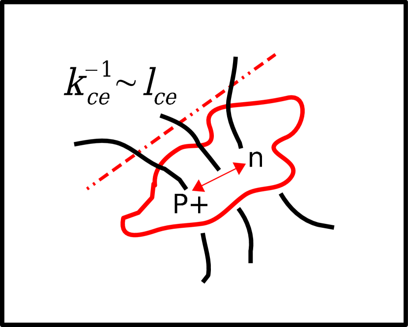
Figure 7: Schematic illustrating the significance of the charge exchange mode, which corresponds to charge exchange interactions per unit area in the computational domain. This mode, being different from the characteristic turbulent mode $k$, is excited naturally when plasma and neutral fluids are coupled in the ISM by charge exchange.

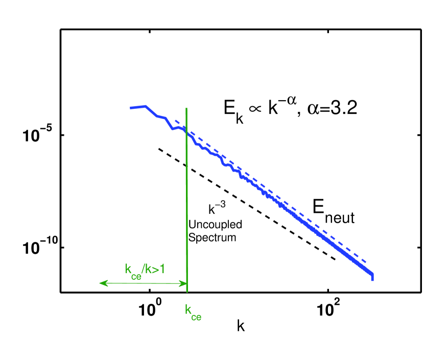
Figure 10: The inertial range turbulent spectrum for a neutral fluid shows a $k^{-3.2}$ spectrum when coupled through charge exchange to a plasma fluid. The spectral index exhibited by this spectrum is larger than that of an ordinary (hydrodynamic) fluid. The latter exhibits a Kolmogorov-like $k^{-3}$ spectrum in the forward cascade regime (drawn schematically). The numerical resolution for our spectral studies is $1024^{2}$ modes in 2D.

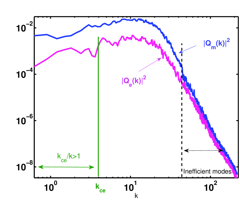
Figure 12: Charge exchange spectrum associated with momentum and energy in both plasma and neutral fluids. Clearly the energy cascades are dominated by large-scale interactions, whereas small scales are not efficient enough to influence the turbulent spectra in the local ISM.

References

- Banks (1966) Banks, P., 1966, Planetary and Space Sci. 14, 1105.
- Basu et al (1994) Basu, S., and Mouschovias, T. Ch. 1994, ApJ, 432, 720.
- Biskamp (2003) Biskamp, D., 2003, Nonlinear MHD Turbulence, Academic Publisher.
- Cho & Lazarian (2003) Cho, J. and Lazarian, A., 2003, MNRAS, 345, 325.
- Elmegreen (1985) Elmegreen, B.G. 1985, ApJ, 299, 196.
- Fite et al (1962) Fite, W. L., Smith, A. C. H., and Stebbings, R. F., 1962, Proc. R. Soc. London, em A. 268, 527.
- Florinski et al (2003) Florinski, V., G. P. Zank, and N. V. Pogorelov (2003), Galactic cosmic ray transport in the global heliosphere, J. Geophys. Res., 108(A6), 1228, doi:10.1029/2002JA009695.
- Florinski et al (2005) Florinski V., G. P. Zank, N. V. Pogorelov (2005), Heliopause stability in the presence of neutral atoms: Rayleigh-Taylor dispersion analysis and axisymmetric MHD simulations, J. Geophys. Res., 110, A07104, doi:10.1029/2004JA010879.
- Goldsmith & Langer (1978) Goldsmith, P.F. and Langer, W.D. 1978, ApJ, 222, 881.
- Gayley et al (1996) Gayley, K., Zank, G. P., Pauls, H. L., Frisch, P. C., and Welty, D. E.: 1997, Astrophys. J. 487, 259.
- Groebner et al (2001) Groebner, R., Madhavi, M. A., Leonard, A. W., Osborne, T. H., Porter, G. D., Colchin, R. J., and Owen, L. W., 2001, GA Report GA-A23856, November; Groebner, R., Baker, D. R., and Burrell, K. H., et al, 2001, 41 No 12, 1789-1802.
- Hill & Dessler (1990) Hill, T. W.; Dessler, A. J., 1990 Geophys. Res. Lett. (ISSN 0094-8276), vol. 17, Sept. 1990, p. 1677-1680.
- Heerikhuisen et al (2006) Heerikhuisen, J.; Florinski, V.; Zank, G. P. 2006, JGR., 111, A06110.
- Ip (1997) Ip, W.-H., 1997, Icarus, Volume 126, Issue 1, pp. 42-57. DOI: 10.1006/icar.1996.5618
- Kolmogorov (1941) Kolmogorov, A. N., 1941, Dokl. Akad. Nauk SSSR, 31, 538.
- Kraichnan (1965) Kraichnan, R. H., 1965, Phys. Fluids, 8, 1385.
- Kudoh et al (2007) Kudoh, T., Basu, S., Ogata, Y., Yabe, T., 2007, MNRAS, 380, 499.
- Kulsrud & Pearce (1969) Kulsrud, R. and Pearce, 1969, ApJ 156, 445.
- Leake et al (2005) Leake, J. E., Arber, T. D., Khodachenko, M. L., 2005, arXiv:astro-ph/0510265v1.
- Li & Nakamura (2004) Li, Z.-Y., Nakamura, F., 2004, ApJ, 609, L83.
- Muller et al (2006) Mueller, H.-R., Frisch, P. C., Florinski, V., and Zank, G. P., 2006, ApJ, 647, 1491.
- Mestel & Spitzer (1956) Mestel, L., Spitzer, L., Jr., 1956, MNRAS, 116, 503.
- McNutt et al (1998) McNutt et al. 1998, JGR, 103, 1905.
- McIvor (1977) McIvor, 1977, MNRAS 178, 85.
- Nakamura & Li (2005) Nakamura, F., Li, Z.-Y., 2005, ApJ, 631, 411.
- Nakano (1979) Nakano, T. 1979, PASJ, 31, 697.
- Oishi & Mac Low (2006) Oishi, J. S. and Mac Low, M., 2006, ApJ, 638, 281.
- Padoan et al (2000) Padoan, P., Zweibel, E., and Nordlund, A., 2000, ApJ, 540, 332.
- Potekhin et al (2005) Potekhin, A. Y.; Lai, Dong; Chabrier, G.; Ho, W. C. G., 2005, Ad. Sp. Res., 35, 1158. DOI:10.1016/j.asr.2004.12.010.
- Pauls et. al (1995) Pauls, H. L., Zank, G. P., and Williams, L. L., 1995, J. Geophys. Res. A11, 21595.
- Scalo (1977) Scalo, J.M. 1977, ApJ, 213, 705.
- Shaikh et al (2006) Shaikh, D. Pogorelov, N. V, and Zank, G. P., 2006, Astronomical Society of the Pacific Conference Series (ASPC), Numerical Modeling of Space Plasma Flows: Astronum-2006, Edited by N. V. Pogorelov and G. P. Zank, 359, 91.
- Shaikh & Zank (2007) Shaikh, D. and Zank, G. P., 2007, AIP Conf. Procs, 932, 111, DOI:10.1063/1.2778952.
- Shebalin & Montgomery (1983) Shebalin, J. V., Matthaeus, W. H., and Montgomery, D. 1983, J. Plasma Phys., 29, 525.
- Shu (1983) Shu, F. H. 1983, ApJ, 273, 202.
- Singh et al (2004) Singh, R., Rogister, A., and Kaw, P., 2004, Phys. Plasma, 11, 129.
- Slavin & Frisch (2006) Slavin, J. D. and Frisch P. C., 2006, ApJ 651, L37-L40.
- Valovie et al (2001) Valovie, M., Fielding, S. J., Carolan, P. G., et al., 2001, Contr. Fusion and Plasma Phys. 25A, 1829.
- Valovie et al (2002) Valovie, M., Carolan, P. G., Fielding, S. J., et al., 2002, Plasma Phys. Contr. Fusion 44, A175.
- Wood et. al (2000) Wood, B. E.; Mueller, H.-R.; Zank, G. P, 2000, ApJ., 542, 493.; Wood, B. E.; Linsky, J. L.; Zank, G. P., 2000, ApJ., 537, 304.
- Zank & Pauls (1996) Zank, G. P. and Pauls, H. L., 1996, Sp. Sci. Rev., 78, 95.
- Zank et al. (1996) Zank, G. P.; Pauls, H. L.; Williams, L. L.; Hall, D. T., 2006, JGR, 101, A10, p. 21639-21656.
- Zank (1999) Zank, G. P., Sp. Sci. Rev., 89, 413-688, 1999.
- Zank et al (2000) Zank, G. P., Lu, J. Y., Rice, W. K. M., and Webb, G. M., 2000, J. Plasma Phys. 64, 507-541.
- Zank et al (2006) Zank, G. P., Mueller, H. -R., Florinski, V., and Frisch, P. C., 2006, Chapter 2 in Solar Journey: Significance of our Galactic Environment for the Heliosphere and Earth, editor P.C. Frisch, Springer, pp. 281-316.
- Zweibel & Josafatsson (1983) Zweibel, E.G. and Josafatsson, K. 1983, ApJ, 270, 511.