Excited states of a string in a time dependent orbifold

Abstract

We present analytical results on the propagation of a classical string in non-zero modes through the singularity of the compactified Milne space. We restrict our analysis to a string winding around the compact dimension of spacetime. The compact dimension undergoes contraction to a point followed by re-expansion. We demonstrate that the classical dynamics of the string in excited states is non-singular in the entire spacetime.

I Introduction

One of the simplest models of the neighborhood of the cosmological singularity (CS), inspired by string/M theory Khoury:2001bz , is the compactified Milne (CM) space. It has been used in the cyclic universe scenario Khoury:2001bz ; Steinhardt:2001vw ; Steinhardt:2001st . Figure 1 shows the two dimensional CM space embedded in three dimensional Minkowski space. It can be specified by the following isometric embedding

$$y^{0}(t,\theta)=t\sqrt{1+r^{2}},~{}~{}~{}~{}y^{1}(t,\theta)=rt\sin(\theta/r),~{}~{}~{}~{}y^{2}(t,\theta)=rt\cos(\theta/r),$$ (1)

where $(t,\theta)\in\mathbb{R}^{1}\times\mathbb{S}^{1}$ and $0<r\in\mathbb{R}^{1}$ is a constant labelling compactifications . One has

$$\frac{r^{2}}{1+r^{2}}(y^{0})^{2}-(y^{1})^{2}-(y^{2})^{2}=0.$$ (2)

Eq. (2) presents two cones with a common vertex at $\>(y^{0},y^{1},y^{2})=(0,0,0)$. The induced metric on (2) reads

$$ds^{2}=-dt^{2}+t^{2}d\theta^{2}.$$ (3)

Generalization of the 2-dimensional CM space to the $d+1$ dimensional spacetime has the form

$$ds^{2}=-dt^{2}+t^{2}d\theta^{2}+\delta_{kl}~{}dx^{k}dx^{l},$$ (4)

where $t,x^{k}\in\mathbb{R}^{1},~{}\theta\in\mathbb{S}^{1}~{}(k=2,\ldots,d)$.

One term in the metric (4) disappears/appears at $t=0$, thus the CM space may be used to model the big-crunch/big-bang type singularity. Orbifolding $\mathbb{S}^{1}$ to the segment gives a model of spacetime in the form of two orbifold planes which collide and re-emerge at $t=0$. Such a model of spacetime was used in Khoury:2001bz ; Steinhardt:2001vw ; Steinhardt:2001st . Our results apply to both choices of topology of the compact dimension.

The CM space is an orbifold due to the vertex at $t=0$. The Riemann tensor components equal $0$ for $t\neq 0$. The singularity at $t=0$ is of removable type: any time-like geodesic with $t<0$ can be extended to some time-like geodesic with $t>0$. However, the extension cannot be unique due to the Cauchy problem at $t=0$ for the geodesic equation (the compact dimension shrinks away and reappears at $t=0$).

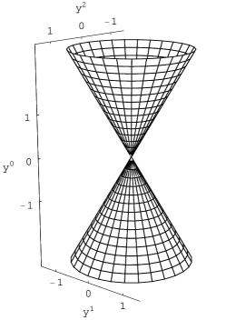
Figure 1: Compactified 2d Milne space embedded in 3d Minkowski space.

The CS plays the key role, in the cyclic model of the evolution of the universe, because it joins each two consecutive classical phases. A reasonable model of the CS should allow for the propagation of an elementary object (particle, string, membrane,…) from the pre-singularity to the post-singularity epoch. If the CS constitutes an insurmountable obstacle for elementary objects, the cyclic evolution cannot be realized.

We have already applied the above criterion for the propagation of a test particle Malkiewicz:2005ii ; Malkiewicz:2006wq and a test string Malkiewicz:2006bw . In what follows (and in Malkiewicz:2006bw ) we examine the dynamics of a string in the so-called winding mode Pioline:2003bs ; Turok:2004gb . It is defined to be a state in which the string is winding around the compact dimension undergoing contraction to a point followed by re-expansion. In Malkiewicz:2006bw we have considered the classical and quantum dynamics of a zero-mode string, i.e. a string in its lowest energy state. Here we present results concerning the propagation of a classical string in non-zero modes, i.e. excited states of a string.

The propagation of a string is described by analytic functions. Thus, it is non-singular in the entire spacetime including the CS. The results we have obtained suggest that the CM space is a promising model of the CS deserving further investigation.

The next section presents the method of finding solutions to the dynamics in the CM space. First, we define 2d CM space by making use of 2d Minkowski space. Then, we recall known solutions in the Minkowski space. Later, we impose the topology and symmetry conditions, specific for the CM space, on the solutions in the Minkowski space. Realization of these conditions leads finally to the solutions in the CM space. As illustrations, we give two specific examples of solutions. We conclude in the last section.

II Dynamics of a string

II.1 Local flatness of the compactified Milne space

The metric corresponding to the compactified Milne space reads

$$g_{\mu\nu}dx^{\mu}dx^{\nu}=-dt^{2}+t^{2}d\theta^{2}+d\overline{x}^{2}.$$ (5)

It is locally flat and can be rewritten in the form of the Minkowski metric, if we make the following change of coordinates

$$x^{0}=t\cosh{\theta},~{}~{}~{}~{}~{}~{}x^{1}=t\sinh{\theta}.$$ (6)

Figure 2 illustrates the compactification of the Milne space. Suppose that $(t,\theta)$ are coordinates of the Milne space, which parameterize the interior of the light-cone. We compactify the Milne space by identification of the points $\theta\sim\theta+\beta$ for some fixed value of $\beta$, where $\theta\in[0,\beta[$. This way the boundaries of the ‘grey’ region become identified.

Figure 2: The interior of the light cones defines the covering space of the compactified Milne space.

In what follows we use the local flatness of (5) to solve the dynamics of a string in the CM space.

II.2 Solutions in the Minkowski space

The string propagation is expressed in terms of embedding functions $x^{\mu}(\tau,\sigma)$, which map the 2d space of the string coordinates into the $(d+1)$-dimensional CM space. An action describing a test string in a fixed background spacetime with metric $g_{\mu\nu}$ may be given by the Polyakov action

$$S_{P}=-\frac{1}{2}\mu\int d\tau d\sigma~{}\sqrt{-\gamma}~{}\gamma^{ab}~{}x_{,a}^{\mu}x^{\nu}_{,b}~{}g_{\mu\nu},$$ (7)

where $(\tau,\sigma)$ are string worldsheet coordinates, $\mu$ is a mass per unit length, $\gamma_{ab}$ is the string worldvolume metric, and $\gamma:=det[\gamma_{ab}]$.

Inserting $\sqrt{-\gamma}~{}\gamma^{ab}:=\eta^{ab}$ (which is a special choice of gauge on the string’s worldsheet) and $g_{\mu\nu}:=\eta_{\mu\nu}$ into (7) gives the Minkowski space case. Variation of $S_{P}$ with respect to $x^{\nu}$ gives

$$\delta S_{P}=\mu\int d\tau d\sigma\;(x^{\mu}_{,\tau}\delta x^{\nu}_{,\tau}-x^{\mu}_{,\sigma}\delta x^{\nu}_{,\sigma})~{}\eta_{\mu\nu}.$$ (8)

The condition $~{}\delta S_{P}=0~{}$ leads to

$$\partial_{\tau}^{2}x^{\mu}-\partial_{\sigma}^{2}x^{\mu}=0,$$ (9)

plus a boundary term. Hence, the string’s propagation in Minkowski space is described by

$$x^{\mu}(\tau,\sigma)=x^{\mu}_{+}(\tau+\sigma)+x^{\mu}_{-}(\tau-\sigma),$$ (10)

$$\partial_{\tau}x^{\mu}\partial_{\tau}x_{\mu}+\partial_{\sigma}x^{\mu}\partial_{\sigma}x_{\mu}=0,~{}~{}~{}~{}~{}~{}\partial_{\tau}x^{\mu}\partial_{\sigma}x_{\mu}=0,$$ (11)

where $x_{\pm}^{\mu}$ are any functions. The equations (11) are just gauge constraints. We can make use of these solutions to construct string solutions in the CM space which wind round the compact dimension, and so can be expressed in terms of a function $\overline{x}(t,\theta)$, where $\overline{x}:=(x^{2},x^{3},\texttt{\ldots},x^{d})$.

II.3 Topology condition

It follows from (6) that the range of this mapping has a non-trivial topology due to the existence of the singular point $(x^{0},x^{1})=(0,0)$. If this point is chosen to correspond to $\tau=0$ then we arrive at the following topology condition

$$x^{0}=f(\tau+\sigma)-f(-\tau+\sigma),~{}~{}~{}~{}~{}x^{1}=g(\tau+\sigma)-g(-\tau+\sigma),$$ (12)

where $f$ and $g$ are any functions.

More generally, we can perform such conformal transformation (i.e., $\sigma_{\pm}\rightarrow\widetilde{\sigma_{\pm}}(\sigma_{\pm})$, where $\sigma_{\pm}=\sigma\pm\tau$) on the solution (10) which leads to $x^{0}=f(\tau+\sigma)-f(-\tau+\sigma)$. One can verify that the solutions for $x^{0}$ which depend only on a single variable, either $\sigma_{+}$ or $\sigma_{-}$, are excluded. It follows from (6) that we have the implication: $(x^{0}=0)\Rightarrow(x^{1}=0)$. This means that for $\tau=0$ we have $x^{1}=0$, which leads to $x^{1}=g(\tau+\sigma)-g(-\tau+\sigma)$.

The map $(\tau,\sigma)\longrightarrow(x^{0},x^{1})$ is everywhere invertible except on the curve $(\tau=0,\sigma\in\mathbb{R})$, because this curve is mapped into the single point $(x^{0},x^{1})=(0,0)$. In this way we have defined a map with its range in a neighborhood of the singularity $x^{0}=0$, having its domain within a global coordinate system on the string’s worldsheet. It is illustrated schematically in Fig 3.

Figure 3: Singular property of the map $(\tau,\sigma)\longrightarrow(x^{0},x^{1})$. The map is invertible for $\tau\neq 0$, and non-invertible for $\tau=0$.

II.4 Symmetry condition

Now, let us impose the symmetry condition on the remaining $x^{k},(k>1)$ embedding functions. Due to the assumption made earlier, $x^{k}$ are functions of $t$ and $\theta$, i.e. $x^{k}(\tau,\sigma)=\widetilde{x}^{k}(t(\tau,\sigma),\theta(\tau,\sigma))$ and are to be periodic in $\theta$. It follows from (12) that

$$\theta=\textrm{arctanh}\Big{(}\frac{g(\sigma_{+})-g(-\sigma_{-})}{f(\sigma_{+})-f(-\sigma_{-})}\Big{)}$$ (13)

$$t=\textrm{sgn}(\tau)~{}\sqrt{(f(\sigma_{+})-f(-\sigma_{-}))^{2}-(g(\sigma_{+})-g(-\sigma_{-}))^{2}}$$ (14)

So the symmetry condition states that $x^{k}=x^{k}_{+}(\sigma_{+})+x^{k}_{-}(\sigma_{-})$ is periodic in $\theta=\textrm{arctanh}(\frac{g(\sigma_{+})-g(-\sigma_{-})}{f(\sigma_{+})-f(-\sigma_{-})})$. In other words, we should determine $x^{k}_{+}$ and $x^{k}_{-}$ from

$$x^{k}_{+}(\sigma_{+})+x^{k}_{-}(\sigma_{-})=\sum_{n}a_{n}^{k}(t)\exp\big{(}\imath\frac{2\pi n}{\beta}\theta\big{)},$$ (15)

where $a_{n}^{k}$ are functions of $t$ whose exact form we will discover below. It may seem to be impossible to satisfy these conditions. One obstacle is due to the fact that on the left-hand side we have a sum of functions of a single variable, while on the right-hand side there is a sum of functions which depend in a rather complicated way on both variables. However, we can compare both sides of (15) at a line. In this way one can rule out one of the variables and compare functions dependent on just a single variable. The procedure rests upon the fact that the dynamics is governed by a second order differential equation (9), and thus it is sufficient to satisfy the symmetry condition by specifying $x^{k}$, $\partial_{t}x^{k}$ on a single Cauchy’s line. We choose it to be the singularity, i.e. the line $\sigma_{+}=-\sigma_{-}$, or equivalently $t=0$. One can check that as $\sigma_{+}+\sigma_{-}\rightarrow 0$, one gets $\theta\rightarrow\textrm{arctanh}(g^{\prime}/f^{\prime})$, where the prime indicates differentiation with respect to an arbitrary parameter.

Our strategy consists in the imposition of the two conditions:

$$\lim_{\sigma_{+}+\sigma_{-}\rightarrow 0}x^{k}=x^{k}_{+}(\sigma)+x^{k}_{-}(\sigma) = \sum_{n}a_{n}^{k}(0)\exp\big{(}\imath\frac{2\pi n}{\beta}\textrm{arctanh}\big{(}\frac{g^{\prime}}{f^{\prime}}\big{)}(\sigma)\big{)},$$ (16)

$$\lim_{\sigma_{+}+\sigma_{-}\rightarrow 0}\partial_{t}x^{k}=\partial_{t}x^{k}_{+}(\sigma)+\partial_{t}x^{k}_{-}(\sigma) = \sum_{n}\dot{a}_{n}^{k}(0)\exp\big{(}\imath\frac{2\pi n}{\beta}\textrm{arctanh}\big{(}\frac{g^{\prime}}{f^{\prime}}\big{)}(\sigma)\big{)}.$$ (17)

In this way we get the following simplifications: (i) as we compare functions on a line we in fact compare functions of a single variable, (ii) since we choose the line $t=0$, we obtain a rather simple form on the right-hand side in the form of a periodic function of $\theta=\arctan(g^{\prime}/f^{\prime})$. The only remaining work to be done is to find the operator $\partial_{t}$ in the limit $~{}\sigma_{+}+\sigma_{-}\rightarrow 0$.

II.4.1 Finding $\partial_{t}$

Let us start with the general expression for $\partial_{t}$

$$\partial_{t} = \frac{\partial_{-}\theta}{\partial_{+}t\partial_{-}\theta-\partial_{-}t\partial_{+}\theta}~{}\partial_{+}-\frac{\partial_{+}\theta}{\partial_{+}t\partial_{-}\theta-\partial_{-}t\partial_{+}\theta}~{}\partial_{-}~{}=:~{}T_{-}\partial_{+}-T_{+}\partial_{-}$$

Now, we evaluate all the components in the above expression:

$$\partial_{+}\tanh(\theta)=\partial_{+}\frac{g(\sigma_{+})-g(-\sigma_{-})}{f(\sigma_{+})-f(-\sigma_{-})}\longrightarrow\frac{1}{2}(\frac{g^{\prime}}{f^{\prime}})^{\prime}~{}\Big{|}_{\sigma_{+}=-\sigma_{-}}$$ (18)

$$\partial_{-}\tanh(\theta)=\partial_{-}\frac{g(\sigma_{+})-g(-\sigma_{-})}{f(\sigma_{+})-f(-\sigma_{-})}\longrightarrow-\frac{1}{2}(\frac{g^{\prime}}{f^{\prime}})^{\prime}~{}\Big{|}_{\sigma_{+}=-\sigma_{-}}$$ (19)

$$\partial_{+}t = \partial_{+}\textrm{sgn}(\sigma_{+}+\sigma_{-})~{}\sqrt{(f(\sigma_{+})-f(-\sigma_{-}))^{2}-(g(\sigma_{+})-g(-\sigma_{-}))^{2}}$$ (20)

$$\longrightarrow \sqrt{(f^{\prime})^{2}-(g^{\prime})^{2}}~{}~{}~{}\Big{|}_{\sigma_{+}=-\sigma_{-}}$$

$$\partial_{-}t = \partial_{-}\textrm{sgn}(\sigma_{+}+\sigma_{-})~{}\sqrt{(f(\sigma_{+})-f(-\sigma_{-}))^{2}-(g(\sigma_{+})-g(-\sigma_{-}))^{2}}$$ (21)

$$\longrightarrow \sqrt{(f^{\prime})^{2}-(g^{\prime})^{2}}~{}~{}~{}\Big{|}_{\sigma_{+}=-\sigma_{-}}$$

One gets

$$\partial_{t}=T_{-}\partial_{+}-T_{+}\partial_{-} \longrightarrow \frac{1}{2\sqrt{(f^{\prime})^{2}-(g^{\prime})^{2}}}(\partial_{+}+\partial_{-})~{}~{}\Big{|}_{\sigma_{+}=-\sigma_{-}}$$ (22)

II.4.2 Application of the two conditions

Let us now study the first condition (16). At the singularity we have

$$x^{k}_{-}(\sigma)+x^{k}_{+}(\sigma) = \sum_{n}a_{n}^{k}(0)\exp\big{(}\imath\frac{2\pi n}{\beta}\textrm{arctanh}\big{(}\frac{g^{\prime}}{f^{\prime}}\big{)}(\sigma)),$$ (23)

which leads to

$$x^{k}(\sigma_{+},\sigma_{-}) = \sum_{n}a_{n+}^{k}\exp\big{(}\imath\frac{2\pi n}{\beta}\textrm{arctanh}\big{(}\frac{g^{\prime}}{f^{\prime}}\big{)}(\sigma_{+})\big{)}$$ (24)

$$+ \sum_{n}a_{n-}^{k}\exp\big{(}\imath\frac{2\pi n}{\beta}\textrm{arctanh}\big{(}\frac{g^{\prime}}{f^{\prime}}\big{)}(-\sigma_{-})\big{)}+F^{k}(\sigma_{+})-F^{k}(-\sigma_{-}),$$

where $a_{n+}^{k}$ and $a_{n-}^{k}=a_{n}^{k}(0)-a_{n+}^{k}$ are constants, and $F^{k}$ is a function to be determined.

The second condition (17) says that if we act on (15) with the $\partial_{t}$ operator and then go to the limit we will end up with the sum of $\exp\big{(}\imath\frac{2\pi n}{\beta}\textrm{arctanh}(\frac{g^{\prime}}{f^{\prime}}(\sigma))\big{)}$ times constant. It means that

$$\frac{(\textrm{arctanh}(\frac{g^{\prime}}{f^{\prime}}))^{\prime}}{{\sqrt{(f^{\prime})^{2}-(g^{\prime})^{2}}}} = C_{1},$$ (25)

$$\frac{(F^{k})^{\prime}}{\sqrt{(f^{\prime})^{2}-(g^{\prime})^{2}}} = C_{2},$$ (26)

where $C_{1}\neq 0$ and $C_{2}$ are constants. From (26) we conclude that

$$x^{k}(\sigma_{+},\sigma_{-}) = \sum_{n}a_{n+}^{k}\exp\big{(}\imath\frac{2\pi n}{\beta}\textrm{arctanh}\big{(}\frac{g^{\prime}}{f^{\prime}}\big{)}(\sigma_{+})\big{)}$$ (27)

$$+ \sum_{n}a_{n-}^{k}\exp\big{(}\imath\frac{2\pi n}{\beta}\textrm{arctanh}\big{(}\frac{g^{\prime}}{f^{\prime}}\big{)}(-\sigma_{-})\big{)}$$

$$+ c_{0}^{k}\textrm{arctanh}\big{(}\frac{g^{\prime}}{f^{\prime}}\big{)}(\sigma_{+})-c_{0}^{k}\textrm{arctanh}\big{(}\frac{g^{\prime}}{f^{\prime}}\big{)}(-\sigma_{-})$$

II.5 Solutions in the compactified Milne space

Now let us consider (25). It does not fully determine the functions $f$ and $g$. This results from the fact that the topology condition (12), which introduced these functions, is invariant under the transformation

$$\sigma_{+}\mapsto\widetilde{\sigma_{+}}=h(\sigma_{+})~{},~{}~{}~{}~{}\sigma_{-}\mapsto\widetilde{\sigma_{-}}=-h(-\sigma_{-})$$ (28)

where $h$ is arbitrary. Thus we fix this gauge by introducing a constraint

$$(\textrm{arctanh}(\frac{g^{\prime}}{f^{\prime}}))^{\prime}=\textrm{const}.$$ (29)

Now from (25) we get

$$f(\sigma) = C\sinh(A\sigma+B)+f_{0},$$ (30)

$$g(\sigma) = C\cosh(A\sigma+B)+g_{0},$$ (31)

where $A$, $B$, $C$, $f_{0}$ and $g_{0}$ are arbitrary constants. We fix the gauge further and put

$$f(\sigma)=q\sinh(\sigma),~{}~{}~{}~{}~{}g(\sigma)=q\cosh(\sigma)$$ (32)

where $q$ is an arbitrary constant.

Therefore, the solution reads

$$x^{0} = q\sinh(\sigma_{+})+q\sinh(\sigma_{-}),$$ (33)

$$x^{1} = q\cosh(\sigma_{+})-q\cosh(\sigma_{-}),$$ (34)

$$x^{k} = \sum_{n}a_{n+}^{k}\exp\big{(}\imath\frac{2\pi n}{\beta}\sigma_{+}\big{)}$$ (35)

$$+ \sum_{n}a_{n-}^{k}\exp\big{(}\imath\frac{2\pi n}{\beta}\sigma_{-}\big{)}+{c_{0}^{k}}(\sigma_{+}+\sigma_{-}),$$

where $k>1$.

These solutions should satisfy the gauge conditions (11), which in the case of the CM space read

$$\partial_{+}x_{k}\partial_{+}x^{k}=q^{2}=\partial_{-}x_{k}\partial_{-}x^{k}.$$ (36)

At this stage, we can determine $\theta$ and $t$, from (13) and (14), as functions of $\sigma_{+}$ and $\sigma_{-}$

$$\theta = \textrm{arctanh}\Big{(}\frac{x^{1}}{x^{0}}\Big{)}=\frac{1}{2}\ln\Big{(}\frac{1+\frac{x^{1}}{x^{0}}}{1-\frac{x^{1}}{x^{0}}}\Big{)}=\frac{1}{2}\ln\Big{(}\frac{e^{\sigma_{+}}-e^{-\sigma_{-}}}{-e^{-\sigma_{+}}+e^{\sigma_{-}}}\Big{)}$$ (37)

$$= \frac{1}{2}\ln(e^{2\sigma})=\sigma$$

$$\frac{t^{2}}{q^{2}} = \big{(}\sinh(\sigma_{+})+\sinh(\sigma_{-})\big{)}^{2}-\big{(}\tanh(\sigma_{+})-\tanh(\sigma_{-})\big{)}^{2}$$

$$= -2+2\big{(}\sinh(\sigma_{+})\sinh(\sigma_{-})+\tanh(\sigma_{+})\tanh(\sigma_{-})\big{)}$$

$$= - 2+\cosh(2\tau)=-2+2\big{(}\sinh(\tau)^{2}+\cosh(\tau)^{2}\big{)}=4\sinh(\tau)^{2}$$ (38)

From the last equation we infer that $\tau=\textrm{arcsinh}(\frac{t}{2q})$. Finally, the solutions as functions of $t$ and $\theta$ have the form

$$x^{k}(t,\theta) = \sum_{n}\Big{(}a_{n+}^{k}e^{\imath\frac{2\pi n}{\beta}\textrm{arcsinh}\big{(}\frac{t}{2q}\big{)}}+a_{n-}^{k}e^{-\imath\frac{2\pi n}{\beta}\textrm{arcsinh}\big{(}\frac{t}{2q}\big{)}}\Big{)}\exp\big{(}\imath\frac{2\pi n}{\beta}\theta\big{)}$$ (39)

$$+ 2c_{0}^{k}\textrm{arcsinh}\Big{(}\frac{t}{2q}\Big{)},$$

where $n$ denotes $n$-th excitation. The number of arbitrary constants in (39) can be reduced by the imposition of the gauge condition (36).

Equation (39) defines the solution corresponding to the compactification of one space dimension to $S^{1}$. The solution corresponding to the compactification to a segment, can be obtained from (39) by the imposition of the condition $x^{k}(t,\theta)=x^{k}(t,-\theta)$, which leads to $a^{k}_{n-}=a^{k}_{(-n)-}$ and $a^{k}_{n+}=a^{k}_{(-n)+}$, where $\theta\in[0,\beta/2]$.

The general solution (39) shows that the propagation of a string through the cosmological singularity is not only continuous and unique, but also analytic. Solution in the CM space is as regular as in the case of the Minkowski space.

The imposition of the gauge constraint (36) on the infinite set of functions given by (39) produces an infinite variety of physical states. This procedure goes exactly in the same way as for a closed string in Minkowski spacetime, but with a smaller number of degrees of freedom due to the condition that the string is winding around the compact dimension.

II.6 Examples of solutions in the CM space

II.6.1 The zero-mode state solution

Let us consider the propagation of a uniformly winding string, i.e. without $\theta$-dependance, in $d+1$ dimensional spacetime

$$x^{k}(t) = d_{0}^{k}+c_{0}^{k}\textrm{arcsinh}\Big{(}\frac{t}{2q}\Big{)},$$ (40)

$$q^{2} = \frac{1}{4}c_{0}^{k}c_{0k},$$ (41)

where the second equation comes from the gauge constraint. Thus we have

$$x^{k}(t)=d_{0}^{k}+c_{0}^{k}\textrm{arcsinh}\Big{(}\frac{t}{\sqrt{c_{0}^{k}c_{0k}}}\Big{)}.$$ (42)

Equation (42) coincides with Eq. (18) of our paper Malkiewicz:2006bw describing the propagation of a string in the zero-mode state, i.e. the lowest energy state.

The velocity of the string, which is calculated with respect to the ‘cosmological time’ $t$, is given by the formula $v=(1+\frac{t^{2}}{c_{0}^{k}c_{0k}})^{-1/2}$, where $k>1$. At the singularity such a string moves with the speed of light.

II.6.2 The solution with non-zero modes

In what follows we present the state with one oscillation mode. The embedding space is five dimensional:

$$x^{2}(t) = d_{0}^{2}+c_{0}^{2}\textrm{arcsinh}\Big{(}\frac{t}{2q}\Big{)}$$

$$x^{3}(t,\theta) = d_{0}^{3}+a\sin\big{(}\frac{2\pi n}{\beta}\big{(}\theta+\textrm{arcsinh}\Big{(}\frac{t}{2q}\Big{)}\big{)}+\delta\big{)}+a\sin\big{(}\frac{2\pi n}{\beta}\big{(}\theta-\textrm{arcsinh}\Big{(}\frac{t}{2q}\Big{)}\big{)}-\delta\big{)}$$

$$x^{4}(t,\theta) = d_{0}^{4}+a\cos\big{(}\frac{2\pi n}{\beta}\big{(}\theta+\textrm{arcsinh}\Big{(}\frac{t}{2q}\Big{)}\big{)}+\delta\big{)}+a\cos\big{(}\frac{2\pi n}{\beta}\big{(}\theta-\textrm{arcsinh}\Big{(}\frac{t}{2q}\Big{)}\big{)}-\delta\big{)}$$

$$q^{2} = \frac{1}{4}(c_{0}^{2})^{2}+\big{(}\frac{2a\pi n}{\beta}\big{)}^{2},$$ (43)

where the last equation is the gauge constraint. The solution can be rewritten in a more compact form (after renaming some of the constants)

$$x^{2}(t) = d_{2}+c~{}\textrm{arcsinh}\Big{(}\frac{t}{\sqrt{c^{2}+(\frac{4a\pi n}{\beta})^{2}}}\Big{)}$$

$$x^{3}(t,\theta) = d_{3}+a\sin\big{(}\frac{2\pi n}{\beta}\theta\big{)}\cos\big{(}\frac{2\pi n}{\beta}\textrm{arcsinh}\Big{(}\frac{t}{\sqrt{c^{2}+(\frac{4a\pi n}{\beta})^{2}}}\Big{)}+\delta\big{)}$$

$$x^{4}(t,\theta) = d_{4}+a\cos\big{(}\frac{2\pi n}{\beta}\theta\big{)}\cos\big{(}\frac{2\pi n}{\beta}\textrm{arcsinh}\Big{(}\frac{t}{\sqrt{c^{2}+(\frac{4a\pi n}{\beta})^{2}}}\Big{)}+\delta\big{)}$$ (44)

Let us calculate the speed of the string

$$v^{2}:=\partial_{t}x^{k}\partial_{t}x_{k}=v^{2}_{\bot}+v^{2}_{\|}$$ (45)

and

$$v^{2}_{\bot} = \frac{c^{2}}{c^{2}+(\frac{4a\pi n}{\beta})^{2}+t^{2}}$$ (46)

$$v^{2}_{\|} = \frac{(\frac{2a\pi n}{\beta})^{2}\sin^{2}(\frac{2\pi n}{\beta}\textrm{arcsinh}(\frac{t}{\sqrt{c^{2}+(\frac{4a\pi n}{\beta})^{2}}})+\delta)}{c^{2}+(\frac{4a\pi n}{\beta})^{2}+t^{2}}$$ (47)

where $v_{\bot}$ is the speed of the center of mass and reaches its maximal value $(1+(\frac{4a\pi n}{\beta c})^{2})^{-1/2}$ at the singularity. The transverse speed is denoted by $v_{\|}$ . It does not depend on $\theta$ since the string is a circle. Its value is a function of both the cosmological time and the phase of the oscillation so the total speed $v$ does not necessarily reach the speed of light at the singularity. The reason is that the string, contrary to the previous example, has some length and therefore nonzero mass even at the singularity.

III Conclusions

The results presented here show that the classical dynamics of a test string in a non-zero mode winding around the compactified dimension is well defined. There are no ambiguities in the dynamics near the singularity as is characteristic of particle dynamics Malkiewicz:2005ii ; Malkiewicz:2006wq . The reason is that a string covers the $\theta$-dimension, so the string does not propagate around this dimension. While a particle can propagate in this dimension, i.e. a particle has one degree of freedom connected with the $\theta$-direction; this is not the case for a string. The property of a string that it is a one dimensional object makes it possible to go through the singularity in an unique way. These results are consistent with the analysis of our previous paper Malkiewicz:2006bw dealing with the string in the zero-mode state.

We have found the solutions in the CM space with two different topologies of the compactified dimension (circle and segment). Both solutions are simply related. The latter CM space presents an interesting model of two ‘end of the world’ branes, and it has been used recently Khoury:2001bz ; Steinhardt:2001vw ; Steinhardt:2001st ; Lehners:2008vx .

The results presented here and in Malkiewicz:2006bw open the door for the examination of the dynamics of extended objects with dimensionality higher than one. Consideration of the winding modes is again preferable. This will be shown in our next paper dealing with the dynamics of a membrane in the compactified Milne space.

We have not considered transitions between exited states during the evolution of the system. That might give some insight into the the backreaction problem. We shall come back to this issue in next papers.

Our results concern the dynamics of a test string. By definition, the test string does not change the background spacetime. A great challenge is examination of the dynamics of a physical string, i.e. a string that may change its state and modify the background spacetime during the evolution of the entire system. Backreaction phenomena cannot be ignored. It has been shown Horowitz:2002mw that, for instance, a single particle added to a time dependent singular orbifold causes the orbifold to collapse into a large black hole, which leads finally to the creation of a big-crunch that would not be followed by a big-bang. In such a case the compactified Milne space would not make sense as a model of the neighbourhood of the cosmological singularity in the context of the cyclic universe scenario. However, the results of Horowitz:2002mw are based mainly on classical general relativity, which is not suitable for understanding the microphysics of a black hole. Complete understanding of the problem requires quantization of the entire system including both string and embedding spacetime. Work is in progress.

References

• (1) J. Khoury, B. A. Ovrut, N. Seiberg, P. J. Steinhardt and N. Turok, “From big crunch to big bang”, Phys. Rev. D 65 (2002) 086007 [arXiv:hep-th/0108187].
• (2) P. J. Steinhardt and N. Turok, “A cyclic model of the universe”, Science 296 (2002) 1436 [arXiv:hep-th/0111030].
• (3) P. J. Steinhardt and N. Turok, “Cosmic evolution in a cyclic universe”, Phys. Rev. D 65 (2002) 126003 [arXiv:hep-th/0111098].
• (4) P. Małkiewicz and W. Piechocki, “The simple model of big-crunch/big-bang transition”, Class. Quant. Grav., 23 (2006) 2963 [arXiv:gr-qc/0507077].
• (5) P. Małkiewicz and W. Piechocki, “Probing the cosmological singularity with a particle”, Class. Quant. Grav., 23 (2006) 7045 [arXiv:gr-qc/0606091].
• (6) P. Malkiewicz and W. Piechocki, “Propagation of a string across the cosmic singularity”, Class. Quant. Grav.  24 (2007) 915 [arXiv:gr-qc/0608059].
• (7) B. Pioline and M. Berkooz, “Strings in an electric field, and the Milne universe”, JCAP 0311 (2003) 007 [arXiv:hep-th/0307280].
• (8) N. Turok, M. Perry and P. J. Steinhardt, “M theory model of a big crunch / big bang transition”, Phys. Rev. D 70 (2004) 106004 [arXiv:hep-th/0408083].
• (9) J. L. Lehners, “Ekpyrotic and Cyclic Cosmology”, Phys. Rept.  465 (2008) 223 [arXiv:0806.1245 [astro-ph]].
• (10) G. T. Horowitz and J. Polchinski, “Instability of spacelike and null orbifold singularities”, Phys. Rev. D 66 (2002) 103512 [arXiv:hep-th/0206228].