Exploiting Low-Dimensional Structure in Astronomical Spectra

Abstract

Dimension-reduction techniques can greatly improve statistical inference in astronomy. A standard approach is to use Principal Components Analysis (PCA). In this work we apply a recently-developed technique, diffusion maps, to astronomical spectra for data parameterization and dimensionality reduction, and develop a robust, eigenmode-based framework for regression. We show how our framework provides a computationally efficient means by which to predict redshifts of galaxies, and thus could inform more expensive redshift estimators such as template cross-correlation. It also provides a natural means by which to identify outliers (e.g., misclassified spectra, spectra with anomalous features). We analyze 3835 SDSS spectra and show how our framework yields a more than 95% reduction in dimensionality. Finally, we show that the prediction error of the diffusion map-based regression approach is markedly smaller than that of a similar approach based on PCA, clearly demonstrating the superiority of diffusion maps over PCA for this regression task.

1 Introduction

Galaxy spectra are classic examples of high-dimensional data, with thousands of measured fluxes providing information about the physical conditions of the observed object. To make computationally efficient inferences about these conditions, we need to first reduce the dimensionality of the data space while preserving relevant physical information. We then need to find simple relationships between the reduced data and physical parameters of interest. Principal Components Analysis (PCA, or the Karhunen-Loève transform) is a standard method for the first step; its application to astronomical spectra is described in, e.g., Boroson & Green (1992), Connolly et al. (1995), Ronen, Aragón-Salamanca, & Lahav (1999), Folkes et al. (1999), Madgwick et al. (2003), Yip et al. (2004a), Yip et al. (2004b), Li et al. (2005), Zhang et al. (2006), Vanden Berk et al. (2006), Rogers et al. (2007), and Re Fiorentin et al. (2007). In most cases, the authors do not proceed to the second step but only ascribe physical significance to the first few eigenfunctions from PCA (such as the “Eigenvector 1” of Boroson & Green). Notable exceptions are Li et al., Zhang et al., and Re Fiorentin et al. However, as we discuss in §4, these authors combine eigenfunctions in an ad hoc manner with no formal methods or statistical criteria for regression and risk (i.e., error) estimation.

In this work we present a unified framework for regression and data parameterization of astronomical spectra. The main idea is to describe the important structure of a data set in terms of its fundamental eigenmodes. The corresponding eigenfunctions are used both as coordinates for the data and as orthogonal basis functions for regression. We also introduce the diffusion map framework (see, e.g., Coifman & Lafon 2006, Lafon & Lee 2006) to astronomy, comparing and contrasting it with PCA for regression analysis of SDSS galaxy spectra. PCA is a global method that finds linear low-dimensional projections of the data; it attempts to preserve Euclidean distances between all data points and is often not robust to outliers. The diffusion map approach, on the other hand, is non-linear and instead retains distances that reflect the (local) connectivity of the data. This method is robust to outliers and is often able to unravel the intrinsic geometry and the natural (non-linear) coordinates of the data.

In §2 we describe the diffusion map method for data parameterization. In §3 we introduce the technique of adaptive regression using eigenmodes. In §4 we demonstrate the effectiveness of our proposed PCA- and diffusion-map-based regression techniques for predicting the redshifts of SDSS spectra. Our PCA- and diffusion-map-based approaches provide a fast and statistically rigorous means of identifying outliers in redshift data. The returned embeddings also provide an informative visualization of the results. In §5 we summarize our results.

2 Diffusion Maps and Data Parameterization

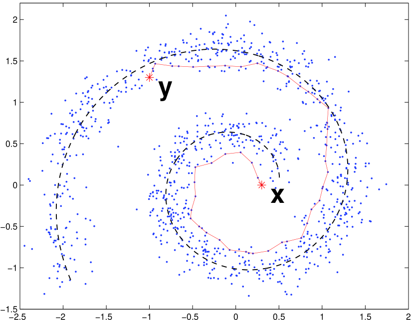
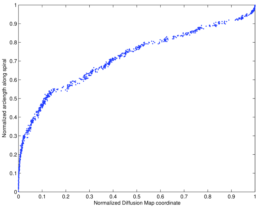
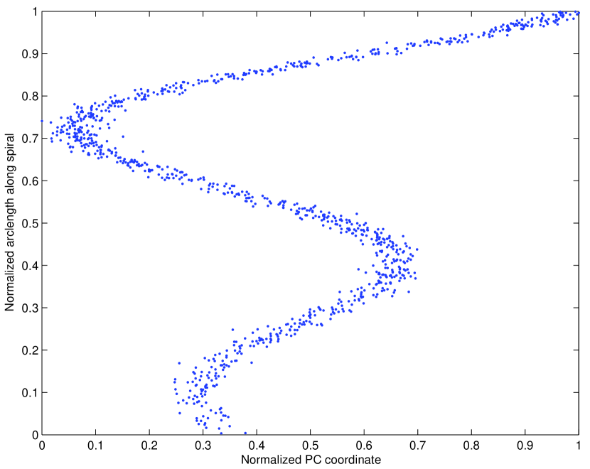
Figure 1: An example of a one-dimensional manifold (dashed line) with Gaussian noise embedded in two or higher dimensions. The path (solid line) from ${\bf x}$ to ${\bf y}$ reflects the natural geometry of the data set which is captured by the diffusion distance between ${\bf x}$ and ${\bf y}$. The plot on the lower left shows that the first diffusion map coordinate is a monotonically increasing function of the arc length of the spiral; this is not the case in the lower right plot, which shows the same relationship for the first PC coordinate.

The variations in a physical system can sometimes be described by a few parameters, while measurements of the system are necessarily of very high dimension; geometrically, the data are points in the $p$-dimensional space $\mathbb{R}^{p}$, with $p$ large. In our case, a data point is a galaxy spectrum, with the dimension $p$ given by the number of wavelength bins ($p\gtrsim 10^{3}$), and a full data set could consist of hundreds of thousands of spectra. To make inference and predictions tractable, one seeks to find a simpler parameterization of the system. The most common method for dimension reduction and data parameterization is Principal Component Analysis (PCA), where the data are projected onto a lower-dimensional hyperplane. For complex situations, however, the assumption of linearity may lead to sub-optimal predictions. A linear model pays very little attention to the natural geometry and variations of the system. The top plot in Figure 1 illustrates this clearly by showing a data set that forms a one-dimensional noisy spiral in $\mathbb{R}^{2}$. Ideally, we would like to find a coordinate system that reflects variations along the spiral direction, which is indicated by the dashed line. It is obvious that any projection of the data onto a line would be unsatisfactory. Results of a PCA analysis of the noisy spiral are shown in the lower-left plot in Figure 1.

In this section, we will use diffusion maps (Coifman & Lafon, Lafon & Lee) — a non-linear technique — to find a natural coordinate system for the data. When searching for a lower-dimensional description, one needs to decide what features to preserve and what aspects of the data one is willing to lose. The diffusion map framework attempts to retain the cumulative local interactions between its data points, or their “connectivity” in the context of a fictive diffusion process over the data. We demonstrate how this can be a better method to learn the intrinsic geometry of a data set than by using, e.g., PCA.

Our strategy is to first define a distance metric $D({\bf x},{\bf y})$ that reflects the connectivity of two points ${\bf x}$ and ${\bf y}$, then find a map to a lower-dimensional space (i.e., a new data parameterization) that best preserves these distances. (As before, a “point” in $p$-dimensional space represents a complete astronomical spectrum of $p$ wavelength bins.) The general idea is that we call two data points “close” if there are many short paths between ${\bf x}$ and ${\bf y}$ in a jump diffusion process between data points. In Figure 1, the Euclidean distance between two points is an inappropriate measure of similarity. If, instead, one imagines a random walk starting at “${\bf x}$,” and only stepping to immediately adjacent points, it is clear that the time it would take for that walk to reach “${\bf y}$” would reflect the length along the spiral direction. This latter distance measure is represented by the solid path from ${\bf x}$ to ${\bf y}$ in Figure 1. We will make this measure of connectivity formal in what follows.

The starting point is to construct a weighted graph where the nodes are the observed data points. The weight given to the edge connecting ${\bf x}$ and ${\bf y}$ is

$$w({\bf x},{\bf y})=\exp\left(-\frac{s({\bf x},{\bf y})^{2}}{\epsilon}\right),$$ (1)

where $s({\bf x},{\bf y})$ is a locally relevant similarity measure. For instance, $s({\bf x},{\bf y})$ could be chosen as the Euclidean distance between ${\bf x}$ and ${\bf y}$ (denoted here $\|{\bf x}-{\bf y}\|$) when ${\bf x}$ and ${\bf y}$ are vectors. But, the choice of $s({\bf x},{\bf y})$ is not crucial, and this gets to the heart of the appeal of this approach: it is often simple to determine whether or not two data points are “similar”, and many choices of $s({\bf x},{\bf y})$ will suffice for measuring this local similarity. The tuning parameter $\epsilon$ is chosen small enough that $w({\bf x},{\bf y})\approx 0$ unless ${\bf x}$ and ${\bf y}$ are similar, but large enough such that the constructed graph is fully connected.

The next step is to use these weights to build a Markov random walk on the graph. From node (data point) ${\bf x}$, the probability of stepping directly to ${\bf y}$ is defined naturally as

$$p_{1}({\bf x},{\bf y})=\frac{w({\bf x},{\bf y})}{\sum_{{\bf z}}w({\bf x},{\bf z})}.$$ (2)

This probability is close to zero unless ${\bf x}$ and ${\bf y}$ are similar. Hence, in one step the random walk will move only to very similar nodes (with high probability). These one-step transition probabilities are stored in the $n$ by $n$ matrix ${\bf P}$. It follows from standard theory of Markov chains (Kemeny & Snell 1983) that, for a positive integer $t$, the element $p_{t}({\bf x},{\bf y})$ of the matrix power ${\bf P}^{t}$ gives the probability of moving from ${\bf x}$ to ${\bf y}$ in $t$ steps. Increasing $t$ moves the random walk forward in time, propagating the local influence of a data point (as defined by the kernel $w$) with its neighbors.

For a fixed time (or scale) $t$, $p_{t}({\bf x},\cdot)$ is a vector representing the distribution after $t$ steps of the random walk over the nodes of the graph, conditional on the walk starting at ${\bf x}$. In what follows, the points ${\bf x}$ and ${\bf y}$ are close if the conditional distributions $p_{t}({\bf x},\cdot)$ and $p_{t}({\bf y},\cdot)$, are similar. Formally, the diffusion distance at a scale $t$ is defined as

$$D_{t}^{2}({\bf x},{\bf y})=\sum_{{\bf z}}\frac{\left(p_{t}({\bf x},{\bf z})-p_{t}({\bf y},{\bf z})\right)^{2}}{\phi_{0}({\bf z})}$$ (3)

where $\phi_{0}(\cdot)$ is the stationary distribution of the random walk, i.e., the long-run proportion of the time the walk spends at node ${\bf z}$. Dividing by $\phi_{0}({\bf z})$ serves to reduce the influence of nodes which are visited with high probability regardless of the starting point of the walk. The distance $D_{t}({\bf x},{\bf y})$ will be small only if ${\bf x}$ and ${\bf y}$ are connected by many short paths with large weights. This construction of a distance measure is robust to noise and outliers because it simultaneously accounts for the cumulative effect of all paths between the data points. Note that the geodesic distance (the shortest path in a graph), on the other hand, often takes shortcuts due to noise.

The final step is to find a low-dimensional embedding of the data where Euclidean distances reflect diffusion distances. A biorthogonal spectral decomposition of the matrix ${\bf P}^{t}$ gives $p_{t}({\bf x},{\bf y})=\sum_{j\geq 0}\lambda_{j}^{t}\psi_{j}({\bf x})\phi_{j}({\bf y})$, where $\phi_{j}$, $\psi_{j}$, and $\lambda_{j}$, respectively, represent left eigenvectors, right eigenvectors and eigenvalues of ${\bf P}$. It follows that

$$D^{2}_{t}({\bf x},{\bf y})~{}=~{}\sum_{j=1}^{\infty}\lambda_{j}^{2t}(\psi_{j}({\bf x})-\psi_{j}({\bf y}))^{2}.$$ (4)

The proof of Equation 4 and the details of the computation and normalization of the eigenvectors $\phi_{j}$ and $\psi_{j}$ are given in Coifman & Lafon and Lafon & Lee. By retaining the $m$ eigenmodes corresponding to the $m$ largest nontrivial eigenvalues and by introducing the diffusion map

$$\Psi_{t}:{\bf x}\mapsto[\lambda_{1}^{t}\psi_{1}({\bf x}),\lambda_{2}^{t}\psi_{2}({\bf x}),\cdots,\lambda_{m}^{t}\psi_{m}({\bf x})]$$ (5)

from $\mathbb{R}^{p}$ to $\mathbb{R}^{m}$, we have that

$$D^{2}_{t}({\bf x},{\bf y})~{}\simeq~{}\sum_{j=1}^{m}\lambda_{j}^{2t}(\psi_{j}({\bf x})-\psi_{j}({\bf y}))^{2}~{}=~{}||\Psi_{t}({\bf x})-\Psi_{t}({\bf y})||^{2}\,,$$ (6)

i.e., Euclidean distance in the $m$-dimensional embedding defined by equation 5 approximates diffusion distance. In contrast, Euclidean distances in PC maps approximate the original Euclidean distances $\|{\bf x}-{\bf y}\|$. Again, consider the example in Figure 1. The plot on the lower left shows that the first diffusion map coordinate is a monotonically increasing function of the arc length of the spiral; this is not the case in the lower right plot, which shows the same relationship for the first PC coordinate. Indeed, the relationship with the first PC coordinate is not even one-to-one.

The choice of the parameters $m$ and $t$ is determined by the fall-off of the eigenvalue spectrum as well as the problem at hand (e.g., clustering, classification, regression, or data visualization). An objective measure of performance should be defined and utilized to find data-driven best choices for these tuning parameters. In this work, the final goal is regression and prediction of redshift. In the next section, we show how the number of coordinates, $m$, can be chosen by cross-validation, once one has defined an appropriate statistical “risk” function. The particular choice of $t$, on the other hand, will not matter in the regression framework, as it will only represent a rescaling of the $m$ selected basis vectors.

3 Adaptive Regression Using Orthogonal Eigenfunctions

Our next problem is how to, in a statistically rigorous way, predict a function $y=r(\mathbf{x})$ (e.g., redshift, age, or metallicity of galaxies) of data (e.g., spectrum $\mathbf{x}$) in very high dimensions using a sample of known pairs (${\bf x},y$). As before, imagine that our data are points in $\mathbb{R}^{p}$, but that the natural variations in the system are along a low dimensional space $\mathcal{X}\subset\mathbb{R}^{p}$. The set $\mathcal{X}$ could, for example, be a non-linear submanifold embedded in $\mathbb{R}^{p}$. In our toy example in Figure 1, $\mathcal{X}$ is the one-dimensional spiral, but the data are observed in $p=2$ dimensions. The key idea is that one may view the eigenfunctions from PCA or diffusion maps (a) as coordinates of the data points, as shown in the previous section, or (b) as forming a Hilbert orthonormal basis for any function (including the regression function $r(\mathbf{x})$) supported on the subset $\mathcal{X}$. Rather than applying an arbitrarily chosen prediction scheme in the computed diffusion or PC space (as in, e.g., Li et al., Zhang et al., and Re Fiorentin et al.), we utilize the latter insight to formulate a general regression and risk estimation framework.

Any function $r$ satisfying $\int r({\bf x})^{2}dx<\infty$, where ${\bf x}\in\mathcal{X}$, can be written as

$$r({\bf x})=\sum_{j=1}^{\infty}\beta_{j}\psi_{j}({\bf x})\,,$$ (7)

where the sequence of functions $\{\psi_{1},\psi_{2},\cdots\}$ forms an orthonormal basis. The choice of basis functions is traditionally not adapted to the geometry of the data, or the set $\mathcal{X}$. Standard choices are, for example, Fourier or wavelet bases for $\mathbf{L}^{2}(\mathbb{R}^{p})$, which are constructed as tensor products of one-dimensional bases. The latter approach makes sense for low dimensions, for example for $p=2$, but quickly becomes intractable as $p$ increases (see, e.g., Bellman 1961 for the “curse of dimensionality”). In particular, note that if a wavelet basis in one dimension consists of $q$ basis functions, and hence requires the estimation of $q$ parameters, the naive tensor basis in $p$ dimensions will have $q^{p}$ basis functions/parameters, creating an impossible inference problem even for moderate $p$. Because this basis is not adapted to $\mathcal{X}$, there is little hope of finding a subset of these basis functions which will do an adequate job of modeling the response.

In this work, we propose a new adaptive framework where the basis functions reflect the intrinsic geometry of the data. Furthermore, we use a formal statistical method to estimate the risk and the optimal parameters in the model. First, rather than using a generic tensor-product basis for the high-dimensional space $\mathbb{R}^{p}$, we construct a data-driven basis for the lower-dimensional, possibly non-linear set $\mathcal{X}$ where the data lie. Let $\{{\psi_{1}},{\psi_{2}},\cdots,{\psi_{n}}\}$ be the orthogonal eigenfunctions computed by PCA or diffusion maps. Our regression function estimate $\widehat{r}({\bf x})$ is then given by

$$\widehat{r}({\bf x})=\sum_{j=1}^{m}\widehat{\beta_{j}}{\psi_{j}}({\bf x}),$$ (8)

where the different terms in the series expansion represent the fundamental eigenmodes of the data, and $m\leq n$ is chosen to minimize the prediction risk that we will now define rigorously.

3.1 Risk: Theory and Estimation

A key aspect of our approach is that the choice of the models is driven by the minimization of a well-justified, objective error criterion which compensates for overfitting. This is critical, as any basis could be utilized to fit the observed data well; this does not provide, however, any assurance that the model applies beyond these data. To begin, we establish the standard stochastic framework within which regression models are assessed. We are given $n$ pairs of observations $(X_{1},Y_{1}),\ldots,(X_{n},Y_{n})$, with the task of predicting the response $Y=r(X)+\epsilon$ at a new data point $X={\bf x}$, where $\epsilon$ represents random noise. (In §4, the response $Y$ is the redshift, $z$, and $X$ is a complete spectrum.) In nonparametric regression by orthogonal functions, one assumes that $r({\bf x})$ is given according to equation (7), with its estimator given by equation (8), with $m\leq n$ where $\{\psi_{j}\}$ is a fixed basis. The primary goal is to minimize the prediction risk (i.e., expected error), commonly quantified by the mean-squared error (MSE)

$$R(m)=\mathbb{E}[Y-\widehat{r}(X)]^{2},$$ (9)

where the average is taken over all possible realizations of $(X,Y)$, including the randomness in the evaluation points $X$, the responses $Y$, and the estimates $\widehat{\beta_{j}}$. Thus, $\mathbb{E}[\cdot]$ averages everything that is random, including the randomness in the evaluation points $X$ and the randomness in the estimates $\widehat{\beta_{j}}$. This leads to protection against overfitting: if a basis function $\psi_{j}$ is unnecessarily included in the model, its coefficient $\widehat{\beta_{j}}$ will only add variability or variance to $\widehat{r}(X)$ and not improve the fit, hence increasing $R(m)$. (On the other hand, as $m$ becomes too small, the estimator becomes increasingly biased, also increasing $R(m)$.) Thus, the ideal choice of $m$ is neither too large, nor too small. In nonparametric statistics, this is dubbed the “bias-variance tradeoff” (see, e.g., Wasserman 2006). A secondary goal is sparsity; more specifically, among the estimators with a small risk, we prefer representations with a smaller $m$.

Since $R(m)$ is a population quantity, one needs to appropriately estimate it from the data. An estimate based on the full data set will underestimate the error and lead to a model with high bias. Here we will use the method of $K$-fold cross-validation (see, e.g., Wasserman) to achieve a better estimate of the prediction risk. The basic idea is to randomly split the data set into $K$ blocks of approximately the same size; $K=10$ is a common choice. For $k=1$ to $K$, we delete block $k$ from the data. We then fit the model to the remaining $K-1$ blocks and compute the observed squared error $\widehat{R}_{(-k)}(m)$ on the $k$th block which was not included in the fit. The CV estimate of the risk is defined as $\widehat{R}_{CV}(m)=\frac{1}{K}\sum_{k=1}^{K}\widehat{R}_{(-k)}(m)$. It can be shown that this quantity is an approximately unbiased estimate of the true error $R(m)$. Thus, we choose the model parameters that minimize the CV estimate $\widehat{R}_{CV}(m)$ of the risk, i.e., we take $m_{\rm opt}=\arg\min\widehat{R}_{CV}(m)$.

Finally, we note that the ideas of CV introduced here generalize to cases where the model parameters are of higher dimension. For example, in the diffusion map case, the risk is minimized over both the bandwidth $\epsilon$ and the number of eigenfunctions $m$. The CV estimate of the risk is implemented in the same fashion, but the search space for finding the minimum is larger. In what follows, the notation will make it clear which model parameters we are minimizing over by writing, for example, $R(\epsilon,m)$.

To summarize, our claim is that the proposed regression framework will lead to efficient inference in high dimensions, as we are effectively performing regression in a lower-dimensional space $\mathcal{X}$ that captures the natural variations of the data, where the optimal dimensionality is chosen to minimize prediction risk in our regression task. Finally, the use of eigenfunctions in both the data parameterization and in the regression formulation provides an elegant, unifying framework for analysis and prediction.

4 Redshift Prediction Using SDSS Spectra

We apply the formalism presented in §§2-3 to the problem of predicting redshifts for a sample of SDSS spectra. Physically similar objects residing at similar redshifts will have similar continuum shapes as well as absorption lines occurring at similar wavelengths. Hence the Euclidean distances between their spectra will be small. The proposed regression framework with diffusion map or PC coordinates provides a natural means by which to predict redshifts. Furthermore, it is computationally efficient, making its use appropriate for large databases such as the SDSS; one can use these predictions to inform more computationally expensive techniques by narrowing down the relevant parameter space (e.g., the redshift range or the set of templates in cross-correlation techniques). Adaptive regression also provides a useful tool for quickly identifying anomalous data points (e.g., objects misclassified as galaxies), galaxies that have relatively rare features of interest, and galaxies whose SDSS redshift estimates may be incorrect.

4.1 Data Preparation

Our initial data sample consists of spectra that are classified as galaxies from ten arbitrarily chosen spectroscopic plates of SDSS DR6 (0266$-$0274 inclusive, and 0286; Adelman-McCarthy et al. 2008). We remove spectra from this sample by applying three cuts. The first is motivated by aperture considerations: we analyze only those spectra with SDSS redshift estimates $z_{\rm SDSS}\geq$ 0.05. To include spectra with $z_{\rm SDSS}<0.05$ would be to add an extra source of variation that would adversely impact regression analysis. The second cut is based on bin flags. To avoid calibration issues observed at both the low and high wavelength ends, we remove the first 100 and last 250 wavelength bins from each spectrum; then we determine what proportion of the remaining 3500 bins are flagged as bad. If this proportion exceeds 10%, we remove the spectrum from the sample; if not, we retain the reduced spectrum for further analysis. We provide details on the third cut below. The application of these cuts reduces our sample size from 5057 to 3835 galaxies.

We further process each spectrum in our sample as follows.

• We replace the flux values in the vicinity of prominent atmospheric lines at 5577 Å, 6300 Å, and 6363 Å with the sample mean of the nine closest bins on either side of each line. The flux errors are estimated by averaging (in quadrature) the standard errors of the fluxes for these bins.

• We similarly replace the flux values in each bin flagged by SDSS as part of an emission line, with flux and flux error estimates based upon the closest 50 bins on either side of the line. (Within this group of 100 bins, we do not include those that are themselves flagged as emission lines.) We do this because highly variable emission line strengths can strongly bias distance calculations.

• Last, after replacing flux values as necessary, we normalize each spectrum to sum to 1 to mitigate variation due to differences in luminosity between similar galaxies at similar redshifts.

In its data reduction pipeline, SDSS estimates spectroscopic redshifts, $z_{\rm SDSS}$, standard errors, $\sigma_{z_{\rm SDSS}}$, and “confidence levels,” CL, the latter of which are functions of the strengths of observed lines (and thus should not be interpreted probabilistically). Lacking knowledge of the true redshifts in our sample, we use $z_{\rm SDSS}$ and $\sigma_{z_{\rm SDSS}}$ to fit our regression model. Since poorly estimated redshifts can bias the model, we divide our data sample into two groups, fitting with only those 2793 galaxies with CL $>$ 0.99. We then use the fitted model to predict redshifts for the other 1042 galaxies. (It is here that we make our third data cut: to avoid issues of extrapolation, we removed 19 of 1061 spectra with CL $\leq$ 0.99 whose SDSS redshift estimates lie outside the range of our training set, i.e. those with $z_{\rm SDSS}>0.50$.) As shown in Figure 2, the distributions of redshifts in our high- and low-CL samples are similar, implying that predicted redshifts for low-CL galaxies from the model built on high-CL galaxies should not be systematically biased.

4.2 Analysis

In this section, we perform both PCA and diffusion map for our sample and predict redshift using the regression model introduced in §3. We provide details on the PCA algorithm in Appendix A.

In the diffusion map analysis, we begin by calculating Euclidean distances between spectra

$$s({\bf x},{\bf y})~{}=~{}\sqrt{\sum_{k}(f_{{\bf x},k}-f_{{\bf y},k})^{2}}\,,$$ (10)

where $f_{{\bf x},k}$ and $f_{{\bf y},k}$ are the normalized fluxes in bin $k$ of spectra ${\bf x}$ and ${\bf y}$, respectively. We use these distances and a chosen value of $\epsilon$ to construct both the weights for the graph (see equation 1) and the transition matrix ${\bf P}$ (see equation 2), from which eigenmodes are generated. Below we discuss how we select the optimal value of $\epsilon$. As stated in §2, the value of the parameter $t$ (see equation 5) is unimportant in the context of regression, as any change in $t$ would be met with a corresponding rescaling of the coefficients $\widehat{\beta}_{j}$ in the regression model, such that predictions are unchanged.

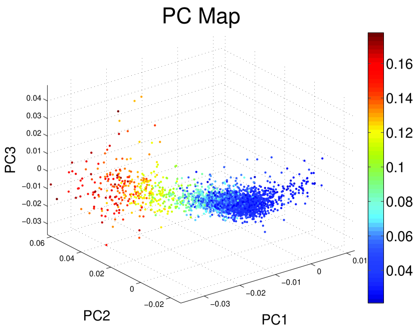
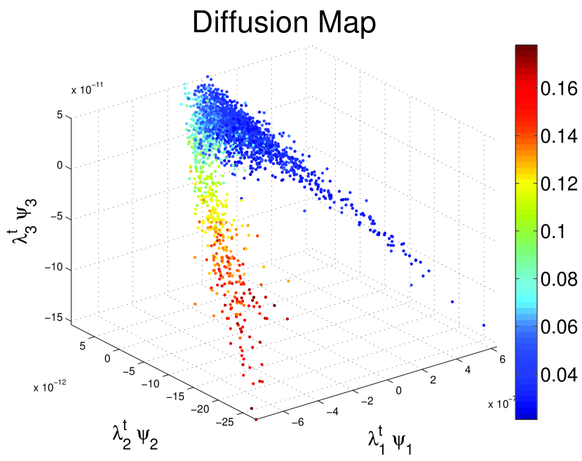
Figure 3: Embedding of our sample of 2793 SDSS galaxy spectra with SDSS $z$ CL $>0.99$ with the first 3 PC and the first 3 diffusion map coordinates, respectively. The color codes for $\log_{10}(1+z_{\rm SDSS})$ values. Both maps show a clear correspondence with redshift.

In Figure 3 we plot the embedding of the 2793 galaxies with CL $>$ 0.99 in the first three PC and diffusion map coordinates (e.g., $\lambda_{i}^{t}\psi_{i}(\cdot)$ in equation 5). We observe that the structure of each of these reparameterizations of the original data corresponds in a simple way to $\log_{10}(1+z_{\rm SDSS})$. These embeddings are a useful way to visualize the data and to qualitatively identify subgroups of data and peculiar data points.

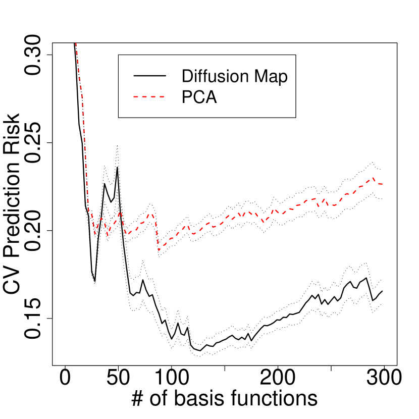
Figure 4: Risk estimates ($\widehat{R}_{CV}$) for regression of $z$ on diffusion map coordinates and PCs. Diffusion map attains a lower risk for almost every number of coordinates in the regression. It also achieves a lower minimum risk as indicated by Table 1. Risk estimates are based on 50 repetitions of 10-fold CV. Thick lines represent mean risk at that model size and thin dotted lines are +/- 1 standard deviation bands.

In the next stage of analysis we use the computed eigenfunctions to predict $z$ for our sample of 3835 galaxies. We regress $z_{\rm SDSS}$ upon the diffusion map (and PC) eigenmodes (cf. equation 8, where $\widehat{r}$ represents our redshift estimates), weighting each data point by the inverse variance of its $z_{\rm SDSS}$, 1/$\sigma_{z_{\rm SDSS}}^{2}$, to account for the uncertainties in $z_{\rm SDSS}$ measurements. We repeat this step for a sequence of $m$ (and $\epsilon$) values, determining the optimal values of each by minimizing the prediction risk $R(\epsilon,m)$, estimated via ten-fold cross-validation (see equation 9 and subsequent discussion). It is in this regression step that we clearly observe the advantage of using diffusion maps over principal components. In Figure 4 we show that diffusion map achieves significantly lower CV prediction risk for most choices of model size $m$ and obtains a much lower minimum $\widehat{R}_{\rm CV}$, i.e., the optimal low-dimensional diffusion map representation of our data captures the trend in $z$ better than the PC representation. Note that the trend in $\widehat{R}_{\rm CV}$ for both PC and diffusion map basis functions is to decrease with increasing model size for small models and to increase with increasing model size for larger models. This is the “bias-variance tradeoff” that was referred to in §3.1: as the size (complexity) of our model increases, the bias of the model decreases while the variance of the model increases. Prediction risk is the sum of the squared bias and variance of a model, explaining the behavior observed in Figure 4: for small models, increasing model size leads to decrease in bias that overwhelms increase in variance while for large models, increase in model size produces minimal decrease in bias and relatively large increase in variance.

In Table 1, we show the parameters for the optimal (minimal $\widehat{R}_{\rm CV}$) diffusion map and PC regression models. Note that since our original data were in 3500 dimensions, our optimal diffusion map model achieves a 96.4% reduction in dimensionality. If we were to choose an arbitrary small model size as is often done in the literature, our prediction risk estimates would be terrible. For example, for model sizes $m=10$ and 20, the CV prediction risks for regression on PC basis functions are 0.305 and 0.209, respectively (compared to optimal value 0.193), while regression on diffusion map basis functions yields $\widehat{R}_{\rm CV}$ of 0.295 and 0.191, respectively (compared to optimal value 0.134). The choice of $\epsilon$ in the diffusion map model also has a significant impact on results. For values of $\epsilon$ that are too small, CV risks are extremely large because the data points are no longer connected in the diffusion process and consequently large outliers occur in the diffusion map parameterization. Likewise, large values of $\epsilon$ yield large prediction risks due to the large weights given to connections between dissimilar data points.

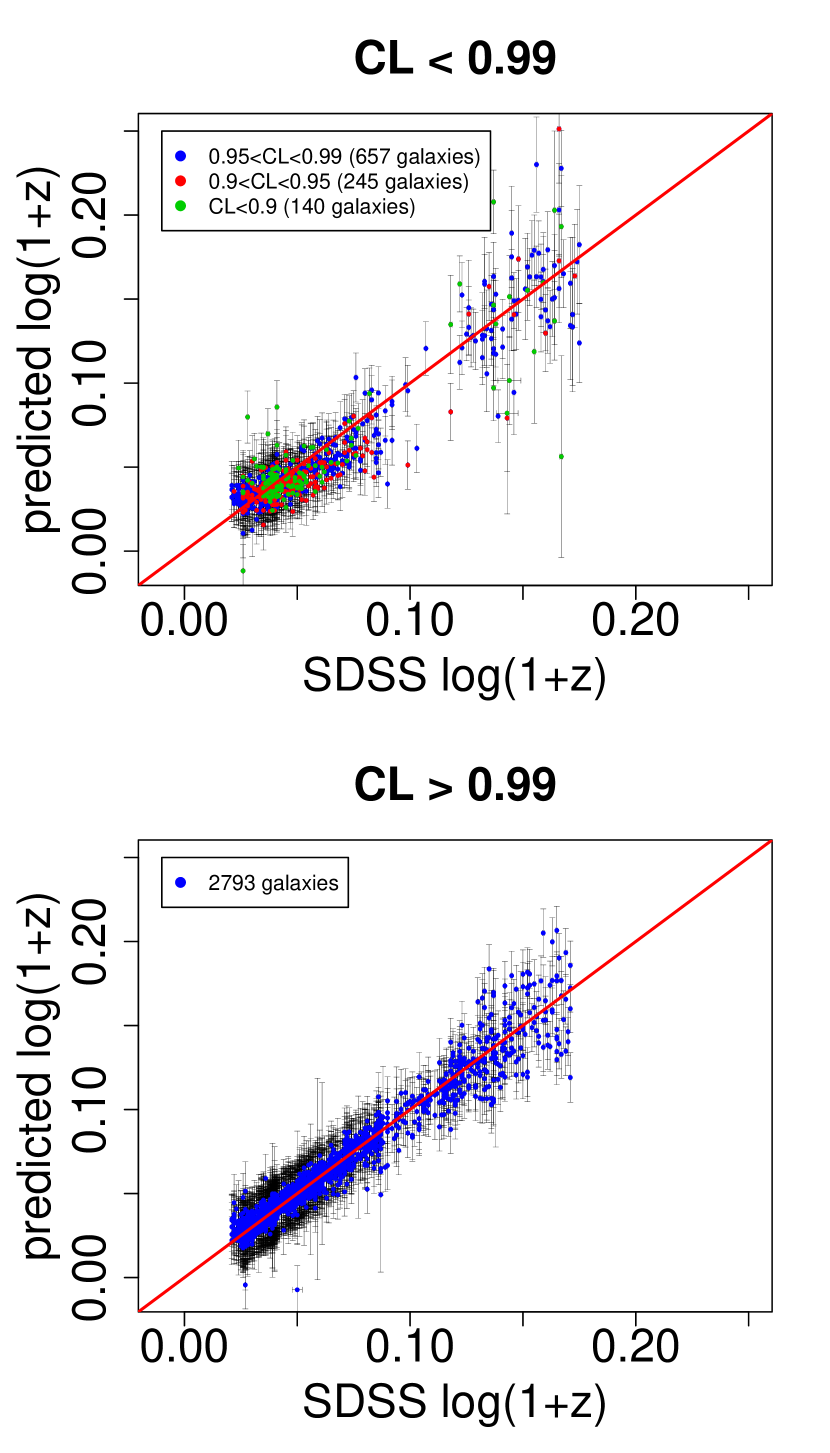
Figure 5: Redshift predictions using diffusion map coordinates for galaxies with SDSS CL $\leq$ 0.99 (top) and CL $>$ 0.99 (bottom), each plotted against $z_{\rm SDSS}$. Error bars represent 95% prediction intervals. Note that CL $\leq$ 0.99 redshift predictions are based on the model trained on CL $>$ 0.99 galaxies while CL $>$ 0.99 predictions are from 10-fold CV on CL $>$ 0.99 galaxies. For most galaxies, our predictions are in close correspondence with SDSS estimates.

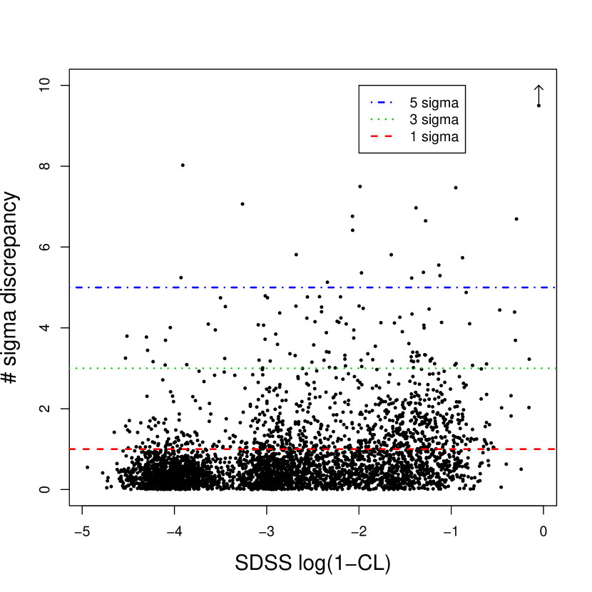
Figure 6: Discrepancy between our predicted redshift values and $z_{\rm SDSS}$ estimates versus log(1-CL). There is a correlation of 0.392 between the amount of discrepancy and 1-CL, meaning that galaxies for which there are large differences between the two redshift estimates tend to be objects whose SDSS redshift confidences are low. Horizontal lines denote 1, 3, and 5 $\sigma$ disparities. Small random perturbations have been added to duplicate log(1-CL) values to visualize galaxies with the same CL. Galaxies with a CL of 1.00 are assigned mean log(1-CL) of -4.

In Figure 5 we plot predictions and prediction intervals for all galaxies in our sample using our optimal diffusion map model. (See Appendix B for a discussion of prediction intervals.) Most of our predictions are in close correspondence with the SDSS estimates. We observe positive correlation in the amount of disparity between our redshift estimates and SDSS estimates versus 1-CL (Figure 6) meaning that galaxies for which our estimates disagree with SDSS estimates are more likely to be galaxies with low CL.

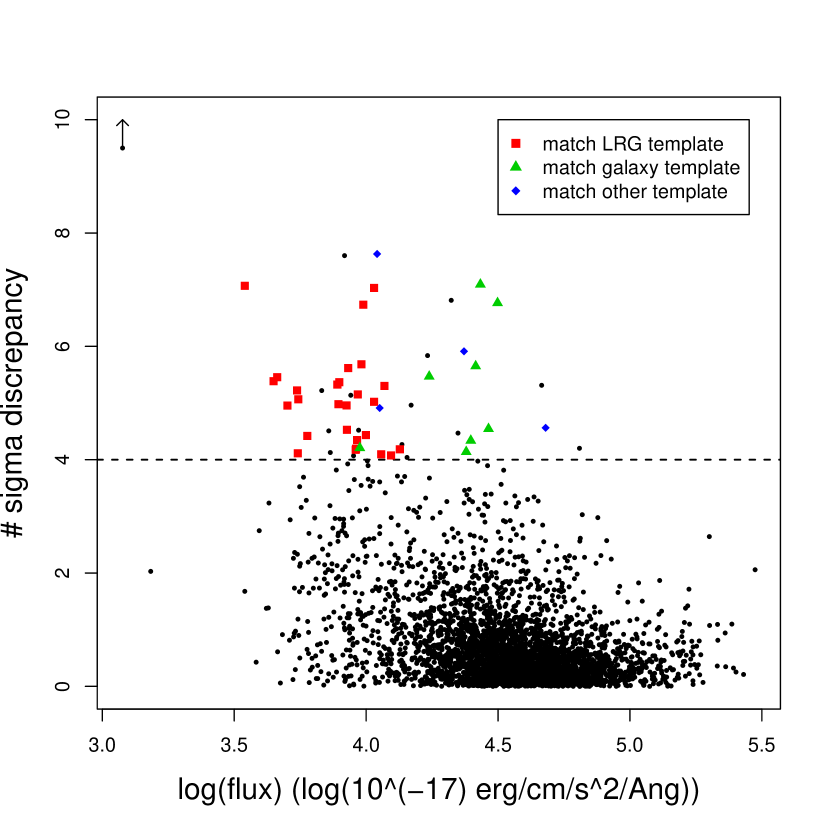
Figure 7: Discrepancy between our predicted redshift values and $z_{\rm SDSS}$ versus log(flux) of the original spectra. There is a correlation of -0.327 between the amount of discrepancy and galaxy brightness. Galaxies can be detected as outliers even if they match well to their SDSS template (in color). Low S/N can cause normal galaxies with correct SDSS redshifts to be labeled as outliers. We also detect several physically interesting objects as outliers (see Figure 8).

There are 54 outliers at the $4\sigma$ level. Visual inspection of their spectra indicates that 39 appear to fit the template assigned by SDSS. Of these, 27 are well-described by the LRG template. In Figure 7 we show that most of the outliers that are well-fit by their SDSS templates are faint objects. A plausible explanation for their classification as outliers is low S/N in their measured spectra. Faint galaxies with strong emission lines will generally have accurate SDSS redshifts but can be outliers in the diffusion map because noisy spectra induce higher Euclidean distances. In a future paper we will introduce a method to account for errors in the original measured data that corrects both for errors in Euclidean distance computations and random errors in the diffusion map coordinates.

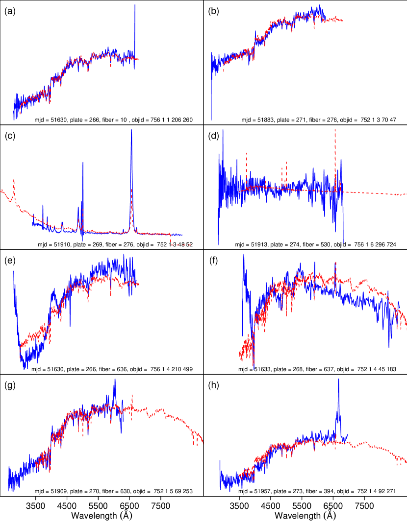
Figure 8: Eight selected outliers with anomalous features. Each spectrum (solid blue) is plotted along with its SDSS template match (dashed red). Spectra are scaled to have the same sum of squared (smoothed) fluxes over the same range of wavelengths. For a thorough discussion of these outliers see §4.2

The 15 other outliers show interesting and/or anomalous features. Four spectra appear to be LRG type galaxies with abnormal emission and/or absorption features, of which at least two are likely attributed to calibration errors (see Figure 8a,b). One spectrum is clearly a QSO (Figure 8c), one shows only sky subtraction residuals (Figure 8d), and two others are obvious mismatches to their SDSS templates due to absorption lines whose depths do not match their assigned template. Four outliers have abnormal bumps (possible continuum jumps due to instrumental artifacts, see Figure 8e,f) that appear like wide emission features. One outlying galaxy has a spectrum that looks like a late-type galaxy with no emission lines, meaning it is likely a K+A post-starburst galaxy. Another outlier has an anomalous emission feature around 6000 Å  in rest frame (Figure 8g). This is a possible lens galaxy, but was not selected by the Sloan Lens ACS Survey (SLACS; Bolton et al.) because the feature in question occurs in close proximity to strong sky lines at 8800 Å . The final outlier has a strong, wide emission feature in the vicinity of H$\alpha$ but has no emission lines anywhere else in the SDSS spectrum (Figure 8h). None of the outlying spectra show conclusive evidence of a wrong SDSS redshift measurement (except for the afore-mentioned sky spectrum, which we detect as a 30 $\sigma$ outlier).

4.3 Comparison With Other Methods

As discussed in §1, many authors have applied PCA to galaxy spectra in an attempt to reduce the dimensionality of the data space, but few attempt to find simple relationships between the reduced data and the physical parameters of interest; these exceptions include Li et al., Zhang et al., and Re Fiorentin et al. In all three cases, the authors use PCA to estimate stellar and/or galactic parameters that are traditionally estimated by laboriously measuring equivalent widths and fluxes of individual lines, just as we have used diffusion map eigenfunctions to estimate redshift, a physical parameter usually estimated through computationally intensive cross-correlation methods. We stress three advantages of our approach over those employed by the above authors: 1) We achieve much lower prediction error using diffusion map coordinates as compared to PCA, 2) we have an objective way of selecting the parameters of the model, and 3) we use a theoretically well-motivated regression model which takes statistical variations of the data into account and which unifies the data parameterization and regression algorithms.

The aim of Li et al. is to estimate, e.g., the velocity dispersion and reddening of a set of approximately 1500 galaxies observed by SDSS. They use PCA in two successive applications. They first apply PCA to the STELIB library to reduce 204 stellar spectra to 24 stellar eigenspectra. These in turn are fit to SDSS DR1 spectra to create a library of 1016 galactic spectra, which are reduced to nine galactic eigenspectra. The authors then regress observed equivalent widths (EW) and fluxes of H$\alpha$ upon these nine eigenspectra. They determine the number of eigenspectra to retain by estimating noise variance in the stellar case and by using the $F$ test to compute the significance of each additional eigenspectrum in spectral reconstruction in the galactic case. The latter criterion however is not well-suited to the task of parameter estimation because the appropriate number of components in the regression model depends on the complexity of the dependence of those parameters as a function of the basis elements, not on the complexity of the original spectra. For example, the dependence of the EW of H$\alpha$ on the PC basis functions may be a simple, smooth function while the flux dependence may be complex, bumpy relationship. In this case, the optimal regression model to predict EW would require fewer basis functions than the optimal model for H$\alpha$ flux prediction. Minimizing CV risk would lead us to choose the correct number of basis functions for each task, while the method of Li et al. would force us to use the same (inappropriate) size for each model.

Zhang et al. attempt to predict stellar parameters by regressing on PC coefficients using a kernel regression model with a variable window width. In their paper, they do not specify how to select the window width (they introduce an arbitrary parameter $\lambda$) or how to choose the correct number of PC basis functions (they use 3). Their choice of a small model size is likely due to the computational and statistical difficulties that characterize kernel regression in high dimensions (Wasserman, 2006).

Re Fiorentin et al. attempt to estimate stellar atmospheric parameters (effective temperature, surface gravity, and metallicity) from SDSS/SEGUE spectra. They use PCA for dimension reduction, but set $m$ to an arbitrary value (e.g., 50). They then use an iterative, non-linear regression model (utilizing the hyperbolic tangent function; see Bailer-Jones 2000), with an error function based on the residual sum-of-squares plus a regularization term (see their equation 2). Again, the choice of the regularization parameter is not justified. We find that when applied to the same data set of galaxy spectra, their model does not achieve lower CV risk than our model for different choices of regularization parameter and model size.

5 Summary

The purpose of this paper is two-fold. First, we introduce the diffusion map method for data parametrization and dimensionality reduction. We show that for the types of high-dimensional and complex data sets often analyzed in the astronomy, diffusion map can yield far superior results than commonly-used methods such as PCA. Moreover, the simple, intuitive formulation of diffusion map as a method that preserves the local interactions of a high-dimensional data set makes the technique easily accessible to scientists that are not well-versed in statistics or machine learning.

Second, we present a fast and powerful eigenmode-based framework for estimating physical parameters in databases of high-dimensional astronomical data. In most astrophysical applications, PCA is used as a data-explorative tool for dimensionality reduction, with no formal methods and statistical criteria for regression, risk estimation and selection of relevant eigenvectors. Here we propose a statistically rigorous, unified framework for regression and data parameterization. Our proposed regression model combines basis functions in a simple and statistically-motivated manner while our clear objective of risk minimization drives the estimation of the model parameters. Again, the simplicity of the proposed method will make it appealing to the non-specialist.

We apply the proposed methodology to predict redshift for a sample of SDSS galaxy spectra, comparing the use of the proposed regression model with PCA basis functions versus diffusion map basis functions. We find that the prediction error for the diffusion-map-based approach is markedly smaller than that of a similar framework based on PCA. Our techniques are also more robust than commonly used template matching methods because they consider the structure of the entire high-dimensional data set when reparametrizing the data. Statistical inferences are based on this learned structure, instead of considering each data point separately in an object-by-object matching algorithm as is currently used by SDSS and commonly employed throughout the astronomy literature. Work in progress extends our approach to photometric redshift estimation and to the estimation of the intrinsic parameters (e.g., mean metallicities and ages) of galaxies.

Appendix A Principal Components Analysis

We first center our data (the normalized spectra with $p$ wavelength bins) so that $\frac{1}{n}\sum_{i=1}^{n}{\bf x}_{i}=0$. The centered observations ${\bf x}_{1},{\bf x}_{2},\ldots{\bf x}_{n}\in\mathbb{R}^{p}$ are then stacked into the rows of an $n\times p$ matrix ${\bf X}$. Note that the sample covariance matrix of $\bf x$ is given by the $p\times p$ matrix ${\bf S}=\frac{1}{n}{\bf X}^{T}{\bf X}$. In Principal Component Analysis (PCA), one computes the eigenvectors of the covariance matrix that correspond to the $m<p$ largest eigenvalues; denote these vectors by ${\bf v}_{1},\ldots,{\bf v}_{m}\in\mathbb{R}^{p}$. In a PC map, the projections of the data onto these vectors are then used as new coordinates; i.e. the PC embedding of data point ${\bf x}_{i}$ is given by the map

$${\bf x}_{i}\mapsto\Psi_{\rm PCA}({\bf x}_{i})=({\bf x}_{i}\cdot{\bf v}_{1},\ldots,{\bf x}_{i}\cdot{\bf v}_{m}).$$

These projections are sometimes referred to as the principal components of ${\bf X}$.

Algorithmically, the PC embedding is easy to compute using a singular value decomposition (SVD) of ${\bf X}$:

$${\bf X=UDV}^{T}.$$

Here ${\bf U}$ is an $n\times p$ orthogonal matrix, ${\bf V}$ is a $p\times p$ orthogonal matrix (where the columns are eigenvectors ${\bf v}_{1},\ldots,{\bf v}_{p}$ of ${\bf S}$), and ${\bf D}$ is a $p\times p$ diagonal matrix with diagonal elements $d_{1}\geq d_{2}\ldots\geq d_{p}\geq 0$ known as the singular values of ${\bf X}$. Since ${\bf XV}={\bf UD}$, the PC embedding of the $i$:th data point in $m$ dimensions is given by the first $m$ elements of the $i$:th row of ${\bf UD}$.

Appendix B Prediction Intervals for Spectroscopic Redshift Estimates

In any one fold of a ten-fold regression analysis, we fit to 90% of the data, generating predictions and prediction intervals for the 10% of the data withheld from the analysis. A prediction interval is not a confidence interval; the former denotes a plausible range of values for a single observation, whereas the latter denotes a plausible range of values for a parameter of the probability distribution function from which that single observation is sampled (e.g., the mean).

Let $\bf X$ and $\bf\tilde{X}$ represent the matrices of independent variables included in, and withheld from, regression analysis, respectively. For instance,

$${\bf\tilde{X}}~{}=~{}\left(\begin{array}[]{cccc}\psi_{1}(x_{1})&\cdots&\cdots&\psi_{m}(x_{1})\\ \vdots&\vdots&\vdots&\vdots\\ \psi_{1}(x_{n})&\cdots&\cdots&\psi_{m}(x_{n})\end{array}\right)\,,$$ (B4)

where $n$ is the number of withheld data and $m$ the number of assumed basis functions. (Here, we leave out factors of $\lambda_{j}^{t}$, which are subsumed into the estimated regression coefficients ${\widehat{\beta}}_{j}$.) The vector of redshift predictions for the withheld data is thus

$${\widehat{z}}~{}=~{}{\bf\tilde{X}}{\widehat{\beta}}\,,$$

where $\widehat{\beta}$ is estimated from ${\bf X}$ while the vector of half-prediction intervals is given by

$$t_{\alpha/2,N-n-2}\widehat{\sigma}\sqrt{{\bf\tilde{X}}\left({\bf X}^{T}{\bf X}\right)^{-1}{\bf\tilde{X}}^{T}+1+\frac{1}{N-n}}\,,$$ (B5)

where $\widehat{\sigma}$ is the estimated standard deviation of the random noise $\epsilon$ in the relationship $Y=r({\bf X})+\epsilon$, estimated from the residuals of the regression of $Y$ upon ${\bf X}$, $t_{\alpha/2,N-n-2}$ is the critical t-value for a two-sided 100(1-$\alpha$)% prediction interval, and $N$ is the total number of data points. Equation (B5) is a multi-dimensional generalization of, e.g., equation (2.26) of Weisberg (2005), taking into account that the mean of $\psi({\bf x})$ is zero.

Figure 2: Distributions of SDSS redshift estimates in our high-CL (top) and low-CL (bottom) samples. We train our regression model using the 2793 high-CL galaxies only, then apply those predictions to the 1042 low-CL galaxies.

Table 1: Parameters of Optimal Regression on $\log_{10}(1+z_{\rm SDSS})$

				Number of Outliers
	$\epsilon_{opt}$	$m_{opt}$	$\widehat{R}_{CV}(\epsilon_{opt},m_{opt})$	$3\sigma$	$4\sigma$	$5\sigma$
Diffusion Map	.0005	127	0.1341	115	54	20
PC	–	88	0.1931	109	55	20

References

- Adelman-McCarthy et al. (2008) Adelman-McCarthy, J. K., et al. 2008, ApJS, 175, 297
- Bailer-Jones (2000) Bailer-Jones, C. A. L. 2000, å, 357, 197
- Bellman (1961) Bellman, R. E. 1961, Adaptive Control Processes (Princeton Univ. Press)
- Boroson & Green (1992) Boroson, T. A., & Green, R. F. 1992, ApJS, 80, 109
- Bolton et al. (2006) Bolton, A. S., et al. 2006, ApJ, 638, 703
- Coifman & Lafon (2006) Coifman, R. R., & Lafon, S. 2006, Appl. Comput. Harmon. Anal., 21, 5
- Connolly et al. (1995) Connolly, A. J., Szalay, A. S., Bershady, M. A., Kinney, A. L., & Calzetti, D. 1995, AJ, 110, 1071
- Folkes et al. (1999) Folkes, S., et al. 1999, MNRAS, 308, 459
- Kemeny & Snell (1983) Kemeny, J. G., & Snell, J. L. 1983, Finite Markov Chains (Springer).
- Lafon & Lee (2006) Lafon, S., & Lee, A. 2006, IEEE Trans. Pattern Anal. and Mach. Intel., 28, 1393
- Li et al. (2005) Li, C., Wang, T.-G., Zhou, H.-Y., Dong, X.-B., & Cheng, F.-Z. 2005, AJ, 129, 669
- Madgwick et al. (2003) Madgwick, D. S., et al. 2003, ApJ, 599, 997
- Re Fiorentin et al. (2007) Re Fiorentin, P., et al. 2007, A&A, 467, 1373
- Rogers et al. (2007) Rogers, B., Ferreras, I., Lahav, O., Bernardi, M., Kaviraj, S., & Yi, S. K. 2007, MNRAS, 382, 750
- Ronen, Aragón-Salamanca, & Lahav (1999) Ronen, S., Aragón-Salamanca, A., & Lahav, O. 1999, MNRAS, 303, 284
- Vanden Berk et al. (2006) Vanden Berk, D. E., et al. 2006, AJ, 131, 84
- Wasserman (2006) Wasserman, L. W. 2006, All of Nonparametric Statistics (New York:Springer)
- Weisberg (2005) Weisberg, S. 2005, Applied Linear Regression (Hoboken:Wiley)
- Yip et al. (2004a) Yip, C. W., et al. 2004, AJ, 128, 585
- Yip et al. (2004b) Yip, C. W., et al. 2004, AJ, 128, 2603
- Zhang et al. (2006) Zhang, J., Wu, F., Luo, A., & Zhao, Y. 2006, ChJAA, 30, 176