ULB-TH/08-23

TAUP 2879-08

A New Holographic Model of Chiral Symmetry Breaking

Stanislav Kuperstein

Physique Théorique et Mathématique, International Solvay Institutes,
Université Libre de Bruxelles, ULB Campus Plaine C.P. 231, B–1050 Brussel, België

Jacob Sonnenschein

School of Physics and Astronomy,
The Raymond and Beverly Sackler Faculty of Exact Sciences,
Tel Aviv University, Ramat Aviv, 69978, Israel.

Abstract

A new family of models of flavour chiral symmetry breaking is proposed. The models are based on the embedding of a stack of $D7$ branes and a stack of anti-$D7$ branes in the conifold background. This family of gravity models is dual to a field theory with spontaneous breaking of conformal invariance and chiral flavour symmetry. We identify the corresponding Goldstone bosons and compute the spectra of massive scalar and vector mesons. The dual quiver gauge theory is also discussed. We further analyse a model where chiral symmetry is not broken.

1 Introduction and Summary

Though the recipe for building the string theory of QCD and hadrons is still a mystery, it should certainly include the ingredients of confinement and flavour chiral symmetry and its spontaneous breakdown. Whereas the realization of the former is easy, the incorporation of the latter is not and is shared only by very few models.

Holographic models are based on taking the near horizon limit of the background produced by large $N_{\textrm{c}}$ branes. Adding $N_{\textrm{f}}$ additional branes, introduces strings stretching between the two type of branes that transform in the fundamental representation of $U(N_{\textrm{c}})\times U_{L}(N_{\textrm{f}})$. Thus, for $N_{\textrm{f}}\ll N_{\textrm{c}}$, when the back-reaction of the additional branes on the background can be neglected, placing a stack of $N_{\textrm{f}}$ $D$-branes in a holographic background associates with adding fundamental quarks in the dual gauge theory. Putting now an additional stack of $N_{\textrm{f}}$ anti $D$-branes results in anti-quarks that transform in the fundamental representation of another $U_{R}(N_{\textrm{f}})$ symmetry which is a gauge symmetry on the new stack of branes. In such a setup the dual gauge theory enjoys the full $U(N_{\textrm{f}})_{L}\times U(N_{\textrm{f}})_{R}$ flavour symmetry. However, if the branes and the anti-branes smoothly merge at some point into a single configuration then only a single $U(N)_{\textrm{D}}$ factor survives. If one can attribute the region where the two separate symmetry groups reside to the UV regime of the dual field theory and where they merge to the IR , then one achieves a “geometrical mechanism” in the gravity model dual of the gauge theory chiral symmetry breakdown.

Such a scenario was derived by adding $D7$ and anti- $D7$ branes to the confining Klebanov-Strassler background (KS) [1] model in [2]. Holomorphic embeddings of $D7$ branes into the KS model which is dual to supersymmetric gauge theory without flavour chiral symmetry breaking were studied in [3, 4] and [5]. The backreaction of the flavour branes (in the so-called un-quenched approximation) have been further investigated in a series of papers [6, 7, 8, 9, 10].

A similar geometrical mechanism was implemented in the Sakai-Sugimoto model [11, 12]. This model incorporates $N_{\textrm{f}}$ $D8$ and $\bar{D}8$ probe branes into Witten’s model [13] which is based on the near extremal $D4$-brane background. An analogous non-critical six dimensional flavoured model was written in [14] and [15] using the construction of [16, 17].

Despite its tremendous success the Sakai-Sugimoto model [11] suffers from various drawbacks which it inherits from Witten’s model [13]. In particular the model is inconsistent in the UV region due to the fact that the string coupling diverges there. In addition the dual field theory is in fact a five dimensional gauge theory compactified on a circle rather than a four dimensional gauge theory. A potential way to bypass these problems is to use as a background the KS model since it is based on $D3$ branes and its dilaton does not run. As mentioned above this was the main idea behind [2]. However, the solution found there for the classical probe profile included an undesired gauge field on the transverse $S^{3}$. On the route to deriving novel solutions of the embedding of $D7$ and anti-$D7$ branes in the KS model, the goal of the present paper is to solve for the embedding of these flavour branes in the context of the un-deformed conifold geometry. The $10d$ solution based on this geometry is known as the Klebanov-Witten (KW) background [18].

The summary of the achievements of the paper are the following:

• We write down the DBI action associated with the embedding of $D7$ branes in the geometry of $AdS_{5}\times T_{11}$. We write the corresponding equations of motion associated with the two angles on the $S^{2}$ which is transverse to the probe branes. We find an analytic solution for the classical embedding. In fact it is a family of profiles along the equator of the $S^{2}$ which are characterised by the minimal radial extension of the probe brane $r_{0}$ and with an asymptotic fixed span of $\sqrt{6}\pi/4$ for the equatorial angle.

• We introduce a Cartesian-like coordinates that enable us to examine the spectrum of scalar mesons associated with the fluctuations of the embedding.

• We identify a massless mode that plays the role of the Goldstone boson associated with the spontaneous breakdown of conformal invariance.

• We compute the spectrum of the massive vector mesons.

• We identify the “pions” associated with the chiral symmetry breaking. They are the zero modes of the gauge fields along the radial direction.

• We write down the quiver that describes the dual gauge field. We also argue why our model includes Weyl and not Dirac fermions as required for a model with chiral symmetry breaking.

• We describe a special case where chiral symmetry is not broken.

The paper is organised as follows: In Section 2 we present the basic setup of the model. Section 3 is devoted to the derivation of the $D7$ probe brane profile solution. We start with a brief review of the conifold geometry. We then write the DBI action and solve the corresponding equation of motion. The spectrum of mesons is extracted in Section 4. We identify the Goldstone mode associated with the spontaneous breaking of conformal invariance and the “pions” that follow from the breaking of the flavour chiral symmetry. We further derive the spectrum of massive vector and scalar mesons. Section 5 is devoted to the dual field theory. We draw the corresponding quiver diagram and discuss the properties of the theory. In Section 6 we discuss a special model where chiral symmetry is not broken.

2 The basic setup

To understand the basic setup of the $D7$-branes in the conifold geometry we first review the setup of the type IIA model of [11]. As was mentioned above it is based on adding to Witten’s model [13] a stack of $N_{\textrm{f}}$ $D8$ branes and a stack of $N_{\textrm{f}}$ anti-$D8$ branes. The $D8$-branes are $9d$ objects, which means that there is only one coordinate transversal to them. Asymptotically this coordinate $x_{4}$ is actually one of world-volume coordinates of the original $D4$ branes. The coordinate is along an $S^{1}$ compactified direction. The submanifold of the background along this direction and the radial direction has a “cigar-like” shape. The radius of the cycle shrinks to zero size at some value of the radial direction $u=u_{\Lambda}$ and diverges asymptotically for large $u$. The profile of the $D8$ probe branes, which is determined by the equations of motion deduced from the DBI action, is of a $U$-shape. It stretches from $x_{4}=-L/2$ at $u\rightarrow\infty$ down to $x_{4}=0$ at a minimum value of $u=u_{0}\geqslant u_{\Lambda}$ and back to $x_{4}=+L/2$ at asymptotic $u$. This shape is obviously in accordance with the fact that on the “cigar” geometry there is no way for the $D8$ branes and the anti $D8$ to end. Their only choice is to merge. Slicing the cigar at large $u$ we have two distinct branches of $D8$ branes with $U(N_{\textrm{f}})_{L}$ gauge field of the left one and $U_{R}(N_{\textrm{f}})$ on the right one. This is the dual picture of the full chiral symmetry at the UV region of the gauge theory. On the other hand down at the tip of the $U$-shape there is only a single $U(N_{\textrm{f}})_{\textrm{D}}$ gauge symmetry which stands for the unbroken global symmetry in the dual gauge theory. Thus the gravity dual of the spontaneous breakdown of chiral symmetry is the $U$-shape structure of the probe branes. A given probe brane profile is characterised by $L\sim 1/\sqrt{u_{0}}$. We mention this relation to contrast the situation that will be found for the $D7$ branes on the conifold. In terms of the dual gauge theory the separation distance $L$ is related to the mass of the mesons. For configurations with $u_{0}\gg u_{\Lambda}$ one finds that the meson mass behaves like $1/L$. Flavour chiral symmetry restoration occurs in QCD at high temperature at the deconfining phase of the theory. In the dual gravity model [19, 20, 21] this phase is described by a distinct geometry of the background where the cigar-like shape describes the submanifold of the Euclidean time direction and the radial direction whereas the $(x_{4},u)$ slice has now a shape of a cylinder that stretches from some minimal value $u=u_{\textrm{T}}$ to infinity. In this geometry the two separate stacks of branes have two options: either to merge like in the low temperature phase or to reach an end separately. The former case translates into a deconfining phase which chiral symmetry breakdown and the latter corresponds to a deconfined phase with a restoration of the full flavour chiral symmetry.

Since we deal with the type IIB supergravity we will need instead a pair of $D7$-branes. Now the transversal space is two-dimensional and analogously to the Sakai-Sugimoto model we need a two-sphere to place the branes on. This is indeed the case as the $T^{1,1}$ base of the conifold has an $S^{3}\times S^{2}$ topology. We now have two different options for the $D7$-brane configuration. One possibility is to place the branes at two separate points on the two-sphere and stretch them to the tip of the conifold, where the two-sphere and the three-sphere shrink. We will refer to this configuration as a $V$-shape. Another possibility is a $U$-shape configuration with $D7$-branes smoothly merging into a single stack at some point $r=r_{0}$ along the radial direction away from the tip. The two options are depicted on Figure 1.

Figure 1: The picture shows two possible $D7$ configurations. In both cases the branes wrap the $S^{3}$ and look like two separate points on the $S^{2}$. The position of this points depends, however, on the radial coordinate $r$. In one case (the $V$-shape) the stacks meet only at the tip of the conifold (the thick curve), while in the other (the $U$-shape) they merge already at $r_{0}>0$ (the thin curve).

We claim that the configuration reaching the tip describes the chiral symmetric phase, while the $U$-shape configuration ending at $r_{0}$ corresponds to the broken chiral symmetry. It looks somewhat perplexing, since instead of a pair of two parallel $D7$-branes we have $D7$-branes that still meet at the tip. Notice, however, that the tip is necessarily a singular point and so the two branches of the $V$-shape are “distinguishable” and correspond to two separate branes. Putting it more bluntly, the tip is a co-dimension six point (both the $S^{2}$ and the $S^{3}$ shrink there!), so the right way to analyse the configuration is to consider its form in the full $10d$ background. The radial coordinate of the conifold combines then with the space-time coordinates to build $AdS_{5}$, which is completely wrapped by the $D7$-branes. The branes wrap also the three-sphere. On the two-sphere, on the other hand, for the $V$-shape the branes look like two separate fixed point, while the $U$-shape corresponds to an arc along the equator. The situation is shown on Figure 2.

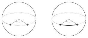
Figure 2: The picture shows two different $D7$-brane profiles on the two-sphere. For the $V$-shape configuration (left) the $D7$-branes are given by two separate fixed points on the $S^{2}$, while for the $U$-shape (right) the position of the two points along the equator depends on $r$ and they are smoothly connected in the middle of the arc for $r=r_{0}$.

An important issue related to the position of the brane on the two-sphere is the amount of supersymmetry preserved by the probe branes. One might think that the two stacks should be located at the antipodal points, let’s say the north and the south pole. In such a case the embedding is holomorphic (see Section 6) and so the setup preserves some supersymmetry. This naïve expectation, however, proves to be wrong, since the configuration with two antipodal points does not solve the equations of motion as we will see in the next section.

3 The configuration

In this section we solve the equations of motion for the $D7$-brane deriving the $U$-shape discussed above. The solution involves a free parameter $r_{0}$ which is just the minimal value of radial coordinate along the profile. As $r_{0}$ goes to zero we will find the $V$-shape configuration. The latter, as we have explained earlier, corresponds actually to a pair of two separate $D7$-branes. We start our journey by reviewing the conifold basics (for a more detailed explanation see [22]).

3.1 Brief review of the conifold geometry

The conifold is a $3d$ complex subspace inside $\mathbb{C}^{4}$ defined by a $2\times 2$ matrix $W$ with vanishing determinant ($\det W=0$). Since the definition is obviously scaling invariant we can fix the radial coordinate of the conifold as:

$$\rho^{2}=\textrm{Tr}\left(W^{\dagger}W\right).$$ (3.1)

Here $\rho$ and the more common radial coordinate $r$ are related by:

$$\rho^{2}=\frac{2^{5/2}}{3^{3/2}}r^{3}.$$ (3.2)

Because $W$ is singular it necessarily has one left and one right null eigenvectors. This in turn implies that $W$ can be re-cast in the form:

$$W=\rho uv^{\dagger},$$ (3.3)

where the vectors $u$ and $v$ both have length one ($u^{\dagger}u=v^{\dagger}v=1$). With these notations the null eigenvectors are $u^{\textrm{T}}\epsilon$ and $\epsilon v^{\star}$, where $\epsilon$ is the $2\times 2$ anti-symmetric tensor. The representation (3.3) is of course not unique, since $W$ is invariant under:

$$u\to e^{i\varphi}u,\qquad v\to e^{i\varphi}v.$$ (3.4)

This way we arrive at a different, but equivalent, definition of the conifold. It can be defined as a Kähler quotient of $\mathbb{C}^{4}$ with the $U(1)_{K}$ gauge charges $(1,1,-1,-1)$. Denoting the $\mathbb{C}^{4}$ coordinates by ${\mathfrak{z}}_{1}$, ${\mathfrak{z}}_{2}$, ${\mathfrak{z}}_{3}$ and ${\mathfrak{z}}_{4}$ we easily find that $u=\sqrt{\rho}({\mathfrak{z}}_{1},{\mathfrak{z}}_{2})^{\textrm{T}}$ and $v=\sqrt{\rho}({\bar{\mathfrak{z}}}_{3},{\bar{\mathfrak{z}}}_{4})^{\textrm{T}}$. Let us now introduce a $2\times 2$ matrix $X$ satisfying:

$$u=Xv.$$ (3.5)

If we also impose an additional constraint saying that $X$ is special and unitary (namely $X\in SU(2)$), then there is an unique solution for (3.5), given by $X=uv^{\dagger}-\epsilon u^{\star}v\epsilon$. Since $X$ is clearly invariant under (3.4) we see that $X$ parameterizes an $S^{3}$. Furthermore, using the Hopf map we realize that the $U(1)_{K}$ transformation (3.4) implies that the unit length vector $v$ alone defines an $S^{2}$. Starting with $X$ and $v$ we can find $u$ and then $W$. We get:

$$W=\rho Xvv^{\dagger}.$$ (3.6)

We conclude that $T^{1,1}$, the base of the conifold (the slice given by $\rho=\textrm{const}$), is uniquely parameterized by $X$ and $v$, so the topology of the base is indeed $S^{3}\times S^{2}$.

Let us now make contact with the explicit $S^{3}\times S^{2}$ conifold coordinates used in the literature [23, 24, 25]. First, note that $vv^{\dagger}$ is a hermitian matrix with eigenvalues $1$ and $0$. We therefore can write:

$$vv^{\dagger}=\mathcal{V}\left(\begin{array}[]{cc}1&0\\ 0&0\end{array}\right)\mathcal{V}^{\dagger},$$ (3.7)

where $\mathcal{V}$ is an $SU(2)$ matrix fixed by $v$ up to the gauge transformation $\mathcal{V}\to\mathcal{V}e^{i\varphi\sigma_{3}}$. Exactly like for $v$ the matrix $\mathcal{V}$ defines an $S^{2}$ by virtue of the Hopf map. Second, we set:

$$\mathcal{V}=e^{\frac{i}{2}\phi\sigma_{3}}e^{\frac{i}{2}\theta\sigma_{2}}.$$ (3.8)

It is always possible to bring the matrix $\mathcal{V}$ to this form using a gauge transformation. We are finally in a position to write the conifold metric in the $S^{3}\times S^{2}$ coordinates:

$$\textrm{d}s_{(6)}^{2}=\textrm{d}r^{2}+\frac{r^{2}}{3}\left(\frac{1}{4}(f_{1}^{2}+f_{2}^{2})+\frac{1}{3}f_{3}^{2}+(\textrm{d}\theta-\frac{1}{2}f_{2})^{2}+(\sin\theta\textrm{d}\phi-\frac{1}{2}f_{1})^{2}\right),$$ (3.9)

where $r$ was introduced in (3.2) and the $1$-forms $f_{i}$ are defined as:

$$\left(\begin{array}[]{c}f_{1}\\ f_{2}\\ f_{3}\end{array}\right)=\left(\begin{array}[]{ccc}0&\cos\theta&-\sin\theta\\ 1&0&0\\ 0&\sin\theta&\cos\theta\end{array}\right)\left(\begin{array}[]{ccc}-\sin\phi&-\cos\phi&0\\ -\cos\phi&\sin\phi&0\\ 0&0&1\end{array}\right)\left(\begin{array}[]{c}w_{1}^{\prime}\\ w_{2}^{\prime}\\ w_{3}^{\prime}\end{array}\right),$$ (3.10)

where $w_{i}$’s are the $SU(2)$ left-invariant Maurer-Cartan one forms:

$$X^{\dagger}\textrm{d}X=\frac{i}{2}\sigma_{i}w_{i}^{\prime}.$$ (3.11)

The two $SO(3)$ matrices in (3.10) reflect the fact that the three-sphere is fibered over the two-sphere. This fiber is trivial as one can easily verify by properly calculating the Chern class of the fiber bundle.

Let us end this section with a remark on the un-deformed conifold symmetries.

First, there is a ${\mathbb{Z}}_{2}$ symmetry that acts as $W\to W^{\textrm{T}}$. On the gauge theory side the symmetry replaces the two $SU(N_{\textrm{c}})$ gauge groups. This fact becomes obvious if following [18] one identifies the Kähler quotient coordinates $\mathfrak{z}_{i}$ with the bi-fundamental chiral superfields $A_{1,2}$ and $B_{1,2}$:

$$(\mathfrak{z}_{1},\mathfrak{z}_{2})=\left(A_{1},A_{2}\right)\qquad\textrm{and}\qquad(\mathfrak{z}_{3},\mathfrak{z}_{4})=\left(B_{1},B_{2}\right).$$ (3.12)

Since under $W\to W^{\textrm{T}}$ we have $(\mathfrak{z}_{1},\mathfrak{z}_{2})\leftrightarrow(\mathfrak{z}_{3},\mathfrak{z}_{4})$, the fields $A_{i}$ and $B_{i}$ are also interchanged. These fields transform in the $(\mathbf{N_{\textrm{c}}},\bar{\mathbf{N_{\textrm{c}}}})$ and $(\bar{\mathbf{N_{\textrm{c}}}},\mathbf{N_{\textrm{c}}})$ representations of the $SU(N_{\textrm{c}})\times SU(N_{\textrm{c}})$ gauge group, and so the ${\mathbb{Z}}_{2}$ interchanges also the $SU(N_{\textrm{c}})$’s. On the other hand, from (3.3) and (3.5) we have $(u,v)\to(v^{\star},u^{\star})$ or alternatively $(X,v)\to(X^{\textrm{T}},(Xv)^{\star})$ under ${\mathbb{Z}}_{2}$. This means that our configuration (Figure 1) which will be discussed in details below, certainly breaks the ${\mathbb{Z}}_{2}$ symmetry. It follows from the fact that $v$ parameterizes the $2$-sphere and the position of the brane on the $S^{2}$ depends only on the radial coordinate and not on $X$, and so the ${\mathbb{Z}}_{2}$ transformation of $v$ is not respected by out setup. This conclusion will play an important rôle in the gauge theory discussion in Section 5.

Second, there is an $SU(2)_{1}\times SU(2)_{2}$ symmetry that acts as $W\to S_{1}WS_{2}^{\dagger}$, where $S_{1}$ and $S_{2}$ are two $SU(2)$ matrices. Under this symmetry the fields $A_{i}$ and $B_{i}$ transform as a doublet of one $SU(2)_{i}$ factor and as a singlet of the other. From (3.6) we see that $(X,v)\to(S_{1}XS_{2}^{\dagger},S_{2}v)$ and so our embedding breaks $S_{2}$, but not $S_{1}$. This fact is expected, since the broken ${\mathbb{Z}}_{2}$ from the previous paragraph interchanges the two $SU(2)_{i}$ symmetries. If, for instance, we were using $u$ (and not $v$) to parameterize the two-sphere, then $S_{1}$ would be broken instead (and not $S_{2}$).

3.2 The $D7$ brane profile

In this paper we will study a $D7$-brane configuration, which spans the space-time coordinates $x_{\mu}$, the radial direction $r$ and the three-sphere parameterized by the forms $f_{i}$ (or alternatively $w_{i}$). The transversal space is given by the two-sphere coordinates $\theta$ and $\phi$. Remarkably, since $w_{i}$ are left-invariant forms, our ansatz preserves one of the $SU(2)$ factors of the global symmetry of the conifold. Based upon this observation, we will assume that $\theta$ and $\phi$ do not depend on the $S^{3}$ coordinates. Since our profile still breaks one $SU(2)$ this assumption should be examined more carefully. Upon expanding the action around the solution we will find that the contributions of the non-trivial $S^{3}$ modes appear only at the second order at the fluctuations. We, therefore, can safely assume that along the classical profile $\theta$ and $\phi$ depend only on the radial coordinate.

The $10d$ metric is:

$$\textrm{d}s_{(10)}^{2}=\frac{r^{2}}{R^{2}}\textrm{d}x_{\mu}\textrm{d}x^{\mu}+\frac{R^{2}}{r^{2}}\textrm{d}s_{(6)}^{2}$$ (3.13)

with the $6d$ metric given by (3.9) and the $AdS_{5}$ radius is $R^{4}=\frac{27}{4}\pi g_{s}N_{\textrm{c}}\ell_{s}^{4}$. Because the KW background has no fluxes except for the $C_{4}$ form the Chern-Simons terms do not contribute and the action consists only of the DBI part:

$$S_{\textrm{DBI}}=-\mu_{7}\int\sqrt{-g_{8}}.$$ (3.14)

Substituting $\theta=\theta(r)$ and $\phi=\phi(r)$ into the metric we find the following Lagrangian:

$$\mathcal{L}\propto r^{3}\left(1+\frac{r^{2}}{6}\left(\theta_{r}^{2}+\sin^{2}\theta\phi_{r}^{2}\right)\right)^{1/2}.$$ (3.15)

Here the subscript _r stands for the derivatives with respect to $r$. The Lagrangian is $SU(2)$ invariant, so we can restrict the motion to the equator of the two-sphere parameterized by $\theta$ and $\phi$. Setting $\theta=\pi/2$ we easily find the solution of the equation of motion:

$$\cos\left(\frac{4}{\sqrt{6}}\phi(r)\right)=\left(\frac{r_{0}}{r}\right)^{4}.$$ (3.16)

There are two branches of solutions for $\phi$ in (3.16) with $\phi\in[-\pi/2,0]$ or $\phi\in[0,\pi/2]$. For $r_{0}=0$ we have two fixed ($r$-independent) solutions at $\phi_{-}=-\frac{\sqrt{6}}{8}\pi$ and $\phi_{+}=\frac{\sqrt{6}}{8}\pi$. The induced $8d$ metric in this case is that of $AdS_{5}\times S^{3}$ as one can verify by plugging $\textrm{d}\phi=\textrm{d}\theta=0$ into (3.9). For non-zero $r_{0}$ the radial coordinate extends from $r=r_{0}$ (for $\phi=0$) to infinity (where $\phi(r)$ approaches one of the asymptotic values $\phi_{\pm}$). The induced metric has no $AdS_{5}\times S^{3}$ structure anymore. As was advertised in the Introduction the $D7$-branes do not reside at the antipodal points on the $(\theta,\phi)$ two-sphere. This is not really surprising since there is a conic singularity at the tip, so the $S^{2}$ does not shrink smoothly. This is in contrast to the low-temperature confining phase of the Sakai-Sugimoto model, where the $x_{4}$ circle smoothly shrinks to zero size resembling the cigar geometry. For a non-orbifolded $\mathbb{R}^{2}$ plane spanned by the polar coordinates $(r,\phi)$ a straight line is given by $\cos(\phi)=r_{0}/r$, where, again, $r_{0}$ is the minimal distance between the origin and the line. The equation (3.16) has a similar form, where the $4$th power and the $4/\sqrt{6}$ factor are both artifacts of the conic singularity of the $6d$ conifold.

Before closing this section let us notice that (3.16) means that we have a family of classical solutions with different parameter $r_{0}$, but with the same boundary values $\phi_{+}$ and $\phi_{-}$ at $r\to\infty$. This implies that once we consider a perturbation theory around the classical profile we should find a massless mode related to the variation of $y_{\textrm{cl}}$ with respect to $r_{0}$. Since for $r_{0}>0$ the induced metric has no $AdS_{5}$ factor, the conformal symmetry of the dual gauge theory should be broken in this case. The massless mode, therefore, is just the Nambu-Goldstone boson of the broken conformal invariance. In the next section we will see that this mode indeed appears in the perturbative expansion.

4 Spectrum of mesons

In this section we will calculate the spectrum of mesons. We will begin with the scalar mesons coming from the variations of the transversal coordinates and will end up with the vector mesons related to the expansion in term of the $D$-brane gauge fields. In both cases we will ignore the non-trivial three-sphere modes.

We start with an observation that the “polar” coordinates $r$ and $\phi$ we used in the profile equation (3.16) do not provide a convenient parameterization of the embedding. As we have already seen, for a fixed value of $r$ the equation (3.16) has two solution corresponding to the two branches of the brane. We therefore cannot use $r$ as an independent coordinate if we want to distinguish between the branches. Moreover, at $r=r_{0}$ the derivative $\partial_{r}\phi(r)$ blows up making the expansion around the classical configuration somewhat problematic. On the other hand, using $\phi$ as an independent coordinate we find that the expansion becomes very complicated and the derivative $\partial_{\phi}r(\phi)$ diverges now at $\phi=\phi_{\pm}$. To summarise, we need a new set of coordinates which properly describes the two branches of the $D7$-brane and also renders the profile (3.16) in a non-singular form.

We found that the following “Cartesian” coordinates do the job:

$$y=r^{4}\cos\left(\frac{4}{\sqrt{6}}\phi\right)\qquad\textrm{and}\qquad z=r^{4}\sin\left(\frac{4}{\sqrt{6}}\phi\right).$$ (4.1)

With the malice of hindsight we have used the same notation as in the original Sakai-Sugimoto paper [11]. Along the configuration (3.16) the coordinate $y$ remains fixed $y_{\textrm{cl}}=r_{0}^{4}$, while $z$ takes all real values. Furthermore, for positive and negative $z$ we have two different branches of the brane. The situation thereof is a generalisation of the coordinates used in [11], where only the $y_{\textrm{cl}}=0$ case was studied. From now on we will use $z$ together with the space-time coordinates $x_{\mu}$ and the Maurer-Cartan forms $f_{i}$ to parameterize the world-volume of the $D7$-brane. In particular, the induced $8d$ metric on the brane is:

$$\textrm{d}s_{(8)}^{2}=\frac{r^{2}}{R^{2}}\textrm{d}x_{\mu}\textrm{d}x^{\mu}+R^{2}\left(\frac{\left(z^{2}+2r_{0}^{8}\right)}{16r^{16}}\textrm{d}z^{2}-\frac{\sqrt{6}r_{0}^{4}}{12r^{8}}\textrm{d}zf_{1}+\frac{1}{6}\left(f_{1}^{2}+f_{2}^{2}\right)+\frac{f_{3}^{2}}{9}\right),$$ (4.2)

where $r=r(z)$ is given by:

$$r^{8}=z^{2}+r_{0}^{8}.$$ (4.3)

In the rest of the section we will use the coordinates $y$ and $z$ to compute the scalar and the vector mesonic spectra.

4.1 Scalar mesons

Plugging $y=y_{\textrm{cl}}+\delta y(x_{\mu},z)$ and $\theta=\theta_{\textrm{cl}}+\delta\theta(x_{\mu},z)$ into the DBI action (3.14), expanding around the classical solution $(y_{\textrm{cl}},\theta_{\textrm{cl}})=(r_{0}^{4},\frac{\pi}{2})$ and integrating over the three-sphere, we arrive at the following action for the fluctuation fields $\delta y(x_{\mu},z)$ and $\delta\theta(x_{\mu},z)$:

$$\delta S_{\textrm{DBI}} = -\frac{2\pi^{2}}{72}\mu_{7}\int\textrm{d}x_{\mu}\textrm{d}z\Bigg{\{}\frac{1}{2}\left(\partial_{z}\delta y\right)^{2}+\frac{R^{4}}{32r^{10}}\left(\partial_{\mu}\delta y\right)^{2}+$$

$$\qquad\qquad+\frac{4}{3}r^{8}\left(\partial_{z}\delta\theta\right)^{2}-\frac{r_{0}^{8}}{2r^{8}}\delta\theta^{2}+\frac{R^{4}}{12r^{2}}\left(\partial_{\mu}\delta\theta\right)^{2}\Bigg{\}},$$

where $r$ is given by (4.3).

Let us start with the $\delta y(x_{\nu},z)$ field. As usual in a meson spectrum calculation we will assume that $\partial_{\mu}\partial^{\mu}\delta y(x_{\nu},z)=M^{2}\,\delta y(x_{\nu},z)$, where $M$ is the $4d$ mass. Introducing a dimensionless variable $x$ and a parameter $\lambda$:

$$x=\frac{z}{r_{0}^{4}}\qquad\textrm{and}\qquad\lambda=\frac{R^{2}M}{r_{0}}$$ (4.5)

we obtain the following Schrödinger-like equation:

$$\partial_{x}^{2}\,\,\delta y+\frac{\lambda^{2}}{16(1+x^{2})^{5/4}}\cdot\delta y=0.$$ (4.6)

In order for the expansion in terms of $\delta y$ to be well-defined the function as well as its derivatives have to be regular (non-divergent) for any value of $x$. The function should also be normalisable at $x\to 0$ and $x\to\pm\infty$. This immediately implies that $\lambda^{2}\geqslant 0$ (and so $M^{2}\geqslant 0$), since otherwise the potential in (4.6) is everywhere positive and so there are no normalisable solutions. Notice also that the potential in (4.6) is even under $x\to-x$. Thus we expect to find pairs of even and one odd solutions. Indeed, near $x=0$ we have $\delta y\sim 1+\mathcal{O}(x^{2})$ or $\delta y\sim x+\mathcal{O}(x^{3})$. On the other hand, for $x\to\infty$ we find that $\delta y\sim 1$ or $\delta y\sim x$. Clearly we have to keep only the former option (the latter solution is also non-normalisable for the action (4.1)).

Before applying a numerical method to solve (4.6) for $M>0$ we would like to point out that the equation is easily solvable for $M=0$. The solutions are $\delta y=1$ and $\delta y=x$. The linear solution is non-normalisable, so we are left only with the first option. This constant solution is exactly the Nambu-Goldstone boson of the broken conformal symmetry we have predicted in the end of the previous section. Consistently this massless mode is $r$-independent since, as was already discussed above, it comes from the $r_{0}$-derivative of the classical configuration $y_{\textrm{cl}}$, which in turn is $r$-independent.

We now want to solve (4.1) with $M>0$ for the entire range of $x$ by gluing one of the two solutions at $x=0$ with the non-divergent solution at infinity. This is, of course, possible only for discrete values of $\lambda_{\mathbf{n}}$, which we found by means of the “shooting technique”. Setting the even ($\delta y(0)=1$, $\delta y^{\prime}(0)=0$) or the odd ($\delta y(0)=0$, $\delta y^{\prime}(0)=1$) boundary conditions at $x=0$, we solved the equation numerically fixing $\lambda$ by allowing only the normalisable (finite $\delta y$) solution for $x\gg 1$. As we have already argued the even (odd) initial conditions at $x=0$ lead to even (odd) solutions of (4.6) and vice versa.

We found:

$$\lambda_{\textrm{n}}^{PC}=4.03^{--},\,5.55^{++},\,7.01^{--},\,8.43^{++},\,9.83^{--},\,11.21^{++}\,\ldots$$ (4.7)

Before explaining the parity ($P$) and charge conjugation ($C$) assignments let us analyse the $\delta\theta(x_{\nu},z)$ field. The same procedure as for $\delta y$ leads to:

$$\partial_{x}\left(\left(1+x^{2}\right)\partial_{x}\delta\theta\right)+\frac{1}{8}\left(\frac{3}{1+x^{2}}+\frac{\lambda^{2}}{2(1+x^{2})^{1/4}}\right)\delta\theta=0.$$ (4.8)

At infinity we have $\delta\theta\sim 1/x$ or $\delta\theta\sim 1$, only the former of which is acceptable, while the latter is now non-normalisable (see the last term in (4.1)). Near $x=0$ we have $\delta\theta\sim 1$ or $\delta\theta\sim x$ exactly like for the $\delta y$ field. Again, both solutions are convergent and give rise to even and odd solutions respectively. For this field the spectrum is:

$$\lambda_{\textrm{n}}^{PC}=2.61^{-+},\,4.39^{+-},\,5.81^{-+},\,8.63^{+-},\,8.63^{-+},\,11.38^{+-}\,\ldots$$ (4.9)

We can now compare these scalar meson spectra to the corresponding spectra of [11] and [15]. We observe that in the latter two models there are scalar states with $0^{++}$ and $0^{--}$ whereas in our model there are states with all the four combinations of $P$ and $C$. In all models there are $0^{--}$ low lying meson states that do not occur in nature.

Let us now explain the parity and the charge conjugation properties of the modes. Our analysis will be very similar to [11]. We can fix the $4d$ parities by requiring the $8d$ action on the $D7$ branes to be $C$ and $P$ invariant. After KK reduction on $S^{3}$ the $5d$ $P$-parity transformation reads $(x_{i},z)\to(-x_{i},-z)$, while the charge conjugation implies both $z\to-z$ and $A\to-A$ (or $A\to-A^{\textrm{T}}$ in the non-Abelian case, see [11]). Since all the fields appear quadratically in the DBI part we will not be able to determine the parities from this part of the action. There is a non-trivial RR $4$-form potential $C_{4}$ in the background, however, and so we have also two Chern-Simons (CS) terms in the action. Both terms do not modify the spectrum calculation, since in the Abelian case they are at least cubic in the field fluctuations, but nevertheless these terms reveal the parity and the charge conjugation transformations of the fields. The first term is:

$$\int F\wedge F\wedge C_{4},\qquad\textrm{with}\qquad C_{4}\sim r^{4}\textrm{d}x_{0}\wedge\textrm{d}x_{1}\wedge\textrm{d}x_{2}\wedge\textrm{d}x_{3}.$$ (4.10)

Here $F$ is the gauge field strength on the brane. This term does not provide any new insight, since it has no $\delta\theta$ or $\delta y$ dependence. The second CS term is due to the Hodge dual of $C_{4}$, which by definition satisfies $\textrm{d}\widetilde{C}_{4}=\star_{10}\textrm{d}C_{4}$. Up to a gauge transformation we have:

$$\widetilde{C}_{4}\sim\cos\theta\,\textrm{d}\phi\wedge\omega_{1}^{\prime}\wedge\omega_{2}\prime\wedge\omega_{3}\prime,$$ (4.11)

where $w_{i}^{\prime}$ are the $SU(2)$ Maurer-Cartan forms we have introduced in Section 3. This CS term yields the following coupling in the $5d$ action:

$$\int F\wedge F\wedge\delta\theta(y_{\textrm{cl}}+\delta y-z\partial_{z}\delta y)\textrm{d}z,$$ (4.12)

where we kept only the two lowest terms in the perturbative expansion. We see that $\delta y$ should transform exactly like $y_{\textrm{cl}}$, which is constant and so clearly both charge conjugation and parity are even. On the other hand , $\delta\theta$ is $C$ even and $P$ odd. The $4d$ parities of the $\delta y$ and $\delta\theta$ modes depend on the solution choice in (4.6) and (4.8). For example, for even solutions of (4.8) we get $0^{-+}$ modes, while odd solutions correspond to $0^{+-}$ modes.

4.2 Vector mesons

Since in this paper we consider only a single probe brane, the first non-trivial contribution in the $F$-expansion of the DBI action yields only the standard $F\wedge\star F$ Abelian term. There is also an $F\wedge F$ term coming from the $C_{4}$ part of the Chern-Simons action, but this term is a total derivative that does not modify the equations of motion. Because we are interested only in the three-sphere independent modes we will ignore gauge fields with legs along the $S^{3}$ and will assume also that the remaining fields depend only on the coordinates $z$ and $x_{\nu}$. The action then reduces to a $5d$ Maxwell action with a $5d$ background metric, which we can find from (4.2) ignoring the $S^{3}$ directions. The action is:

$$S=-T^{\prime}\int\textrm{d}x^{4}\textrm{d}z\big{(}C(z)F_{\mu\nu}F^{\mu\nu}+2D(z)F_{\mu z}F^{\mu}_{z}\big{)},$$ (4.13)

where we absorbed various numerical and dimensionful constants in $T^{\prime}$, the space-time indices $\mu$, $\nu$ are contracted with the Minkowskian metric and:

$$C(z)=\frac{R^{4}}{(z^{2}+r_{0}^{8})^{1/2}}\propto\sqrt{-g_{8}}\left(g_{8}^{\mu\nu}\right)^{2}\,\,\,\textrm{and}\,\,\,\,D(z)=16(z^{2}+r_{0}^{8})^{3/4}\propto\sqrt{-g_{8}}g_{8}^{\mu\nu}g_{8}^{zz}.$$ (4.14)

Here $g_{8}$ stands for the $8d$ metric (4.2). Next we consider the following mode decomposition of the fields:

$$A_{\mu}(x,z)=\sum_{\mathbf{n}}a^{\mathbf{n}}_{\mu}(x)\alpha^{\mathbf{n}}(z)\quad\textrm{and}\quad A_{z}(x,z)=\sum_{\mathbf{n}}b^{\mathbf{n}}(x)\beta^{\mathbf{n}}(z).$$ (4.15)

With this decomposition the field strength reads:

$$F_{\mu\nu}=\sum_{\mathbf{n}}f^{\mathbf{n}}_{\mu\nu}(x)\alpha^{\mathbf{n}}(z)\quad\textrm{and}\quad F_{\mu z}=\sum_{\mathbf{n}}\left(\partial_{\mu}b^{\mathbf{n}}(x)\beta^{\mathbf{n}}(z)-a^{\mathbf{n}}_{\mu}(x)\partial_{z}\alpha^{\mathbf{n}}(z)\right),$$ (4.16)

where $f_{\mu\nu}=\partial_{\mu}a_{\nu}-\partial_{\nu}a_{\mu}$. Substituting this back into the action (4.13) we receive:

$$S = -T^{\prime}\int\textrm{d}x^{4}\textrm{d}z\sum_{\mathbf{m},\mathbf{n}}\Big{(}C(z)f_{\mu\nu}^{\mathbf{n}}{f^{\mathbf{n}}}^{\mu\nu}\alpha^{\mathbf{n}}\alpha^{\mathbf{m}}+$$

$$\quad+2D(z)\left(\partial_{\mu}b^{\mathbf{n}}\partial^{\mu}b^{\mathbf{m}}\beta^{\mathbf{n}}\beta^{\mathbf{m}}+a^{\mathbf{n}}_{\mu}a^{\mathbf{m}\mu}\partial_{z}\alpha^{\mathbf{n}}\partial_{z}\alpha^{\mathbf{m}}-2\partial_{\mu}b^{\mathbf{n}}a^{\mathbf{m}\mu}\beta^{\mathbf{n}}\partial_{z}\alpha^{\mathbf{m}}\right)\Big{)}.$$

Following [11] we first consider the equation of motion and the normalization condition for $\alpha^{\mathbf{n}}(z)$:

$$-\frac{1}{C(z)}\partial_{z}\left(D(z)\partial_{z}\alpha^{\mathbf{n}}(z)\right)=M_{\mathbf{n}}^{2}\alpha^{\mathbf{n}}(z)\,\,\,\textrm{and}\,\,\,\,T^{\prime}\int_{-\infty}^{\infty}\textrm{d}zC(z)\alpha^{\mathbf{n}}(z)\alpha^{\mathbf{m}}(z)=\delta_{\mathbf{n}\mathbf{m}}.$$ (4.18)

Here the equation of motion is derived from the third term in (4.2), while the normalization is dictated by the first term. Using both equations in (4.2) we get rid of the $z$-dependence of the first and the third terms obtaining this way the standard $4d$ kinetic and mass term for the gauge fields $a^{\mathbf{n}}_{\mu}$’s. We have meanwhile ignored the $\beta^{\nu}(z)$ modes. The reason for that is the absence of a kinetic term for these modes. This means that we only have to impose a right normalization for $\beta^{\mathbf{n}}(z)$’s. Remarkably, the following simple substitution:

$$\beta^{\mathbf{n}}(z)=\frac{\partial_{z}\alpha^{\mathbf{n}}(z)}{M_{\mathbf{n}}}$$ (4.19)

does the job. With the help of (4.18) the second term in (4.2) provides a standard kinetic term $\partial_{\mu}b^{\mathbf{n}}\partial^{\mu}b^{\mathbf{n}}$ for the scalar fields $b^{\mathbf{n}}$’s, while the last term in (4.2) reduces to the form $-2\partial_{\mu}b^{\mathbf{n}}{a^{\mathbf{n}}}^{\mu}$. It turns out that both terms can be eliminated by the gauge transformation:

$$a_{\mu}^{\mathbf{n}}\longrightarrow a^{\mathbf{n}}_{\mu}+\frac{\partial_{\mu}b^{\mathbf{n}}}{M_{\mathbf{n}}}.$$ (4.20)

This seems to complete the analysis, meaning that there are no scalars in the final $4d$ action, only the gauge fields $a^{\mathbf{n}}_{\mu}$. Yet there is a trap here: we just overlooked an additional normalisable mode $\beta^{\mathbf{0}}(z)$, which is orthogonal to all other modes ${\beta^{\mathbf{n}}(z)\propto\partial_{z}\alpha^{\mathbf{n}}(z)}$ for all $\mathbf{n}\geqslant 1$ with respect to the scalar product defined by the second term in (4.2). This mode is $\beta^{\mathbf{0}}(z)=\kappa/D(z)$. We can easily check that:

$$\int_{-\infty}^{\infty}\textrm{d}zD(z)\beta^{\mathbf{0}}(z)\beta^{\mathbf{n}}(z)=\frac{\kappa}{M_{\mathbf{n}}}\int_{-\infty}^{\infty}\textrm{d}z\partial_{z}\alpha^{\mathbf{n}}(z)=0.$$ (4.21)

The constant $\kappa$ has to be fixed by the normalization of the mode $\beta^{\mathbf{0}}(z)$:

$$\frac{1}{\kappa^{2}}=4T^{\prime}\int_{-\infty}^{\infty}\frac{\textrm{d}z}{D(z)}.$$ (4.22)

Plugging $\beta^{\mathbf{0}}(z)$ into the action we find an additional scalar kinetic term $\partial^{\mu}b^{\mathbf{0}}\partial_{\mu}b^{\mathbf{0}}$ that cannot be eliminated by any gauge transformation. To summarise, we find that the $4d$ action consists of the massive gauge fields $\alpha_{\mu}^{\mathbf{n}}$ and the massless scalar $b^{\mathbf{0}}$:

$$S_{4d}=-\int\textrm{d}x^{4}\left(\frac{1}{2}\partial^{\mu}b^{\mathbf{0}}\partial_{\mu}b^{\mathbf{0}}+\sum_{\mathbf{n}\geqslant 1}\left(\frac{1}{4}f_{\mathbf{n}}^{\mu\nu}f^{\mathbf{n}\mu\nu}+\frac{1}{2}M_{\mathbf{n}}^{2}a_{\mu}^{\mathbf{n}}a^{\mathbf{n}\mu}\right)\right).$$ (4.23)

Following the discussion in Introduction we will identify $b^{\mathbf{0}}$ as the Goldstone boson of the broken chiral symmetry. This implies that the we should anticipate this mode only for $r_{0}>0$, namely for the $U$-shape of two smoothly merging $D7$-branes, but not for $r_{0}=0$ which corresponds to the $V$-shape of two separate branes. The answer to this puzzle is encoded in the convergence of the integral in (4.22). For $r_{0}=0$ we have $D(z)=16\cdot z^{-3/2}$ and the integral (4.22) diverges at $z=0$, so, as predicted, the massless mode does not exist for the $V$-shape. On the other hand, the integral is finite for $r_{0}>0$ as expected.

Our last goal in this section is to find the spectrum of the massive vector mesons. To this end we have to solve the first equation in (4.18). Proceeding the same way like with the scalar mesons we obtain the following results:

$$\lambda_{\textrm{n}}=2.03^{++},\quad 3.32^{--},\quad 4.71^{++},\quad 6.05^{--},\quad 7.41^{++},\quad 8.76^{--},\ldots$$ (4.24)

Here the the parity and the charge conjugation properties are identified exactly like in the Sakai-Sugimoto model [11]. In particular, the massless mode $b^{\mathbf{0}}$ is $0^{-+}$.

5 The dual gauge theory

In this section we will analyse the dual gauge theory. As we have already mentioned in Section 3 the Kähler quotient coordinates $\mathfrak{z}_{i}$ of the conifold correspond to the chiral bi-fundamentals $A_{i}$ and $B_{i}$ in the quiver gauge theory. To be more specific, we have $u\propto\left(A_{1},A_{2}\right)^{\textrm{T}}$ and $v^{\star}\propto\left(B_{1},B_{2}\right)^{\textrm{T}}$, see (3.12). In this paper we used $X\in SU(2)$ and $v$ to parameterize the three- and the two-spheres of the conifold and our embedding looks like two separate points on $S^{2}$. The position of these points depends on the radial coordinate for $r_{0}>0$ (broken conformal and chiral symmetries) and is fixed for $r_{0}=0$ (un-broken symmetries).

For the embedding to be supersymmetric (namely to preserve four out of the eight supercharges of the background) it has to be given by a holomorphic function [26] (see also [27]). It is easy to check that for $r_{0}>0$ the embedding is explicitly non-holomorphic. Let us now address the $r_{0}=0$ case. Since the conifold inherits the complex structure of ${\mathbb{C}}^{4}$ we conclude that the $r_{0}=0$ embedding is supersymmetric if and only if one has $B_{1}=0$ or $B_{2}=0$ along the brane (which is the same as $\mathfrak{z}_{3}=0$ or $\mathfrak{z}_{4}=0$). This, however, describes two antipodal points on the 2-sphere parameterized by $v$ and we have demonstrated that there is no such solution. Instead we found that the angle difference is $\frac{\sqrt{6}}{4}\pi$. To conclude, the embedding breaks supersymmetry for any $r_{0}$.

Figure 3: The quiver diagram of the supersymmetric embedding elaborated in [3]. Here dots denote the gauge groups and the boxes correspond to the global flavour symmetries. Notice that there is no anomaly, as for each node the number of incoming and outgoing arrows are equal.

The fact that there is no supersymmetric antipodal configuration matches, to some extent, the quiver gauge theory expectations. To see this, let us first consider the holomorphic embedding studied in [3]. In terms of the bi-fundamentals it is given by:

$$A_{1}B_{1}=\mu$$ (5.1)

and we will put $\mu=0$ for simplicity. In this case it is straightforward to find the quiver diagram and the flavour part of the superpotential. The quiver of Figure 3 and the additional part in the superpotential is [3]:

$$\Delta W=q_{2}B_{1}\widetilde{q}_{1}+q_{1}A_{1}\widetilde{q}_{2}.$$ (5.2)

Higgsing the fields $A_{1}$ and $B_{1}$ one finds massive quarks, while the requirements for the quarks to be massless leads to the $A_{1}B_{1}=0$ embedding (see [5, 3]).

Notice now that the same approach will not work for the $B_{1}B_{2}=0$ embedding, which describes $D7$ and anti-$D7$ at the antipodal points on the two-sphere (see Footnote 7). This is because in order to simultaneously include the terms ${q_{2}}B_{1}\widetilde{q}_{1}$ and $\widetilde{q}_{2}B_{2}q_{1}$ in the superpotential we will have to invert the arrows of $\widetilde{q}_{2}$ and $q_{1}$ in the diagram on Figure 3. This, however, will produce an anomalous quiver diagram, since the number of incoming and outgoing arrows (for either node $1$ or $2$) will be different. We see that as expected we cannot add flavours to the gauge theory in a way that will correspond to the antipodal brane configuration.

Figure 4: A quiver diagram that doesn’t respect the ${\mathbb{Z}}_{2}$ symmetry.

We argued in Section 3 that our $D7$-brane configuration breaks the ${\mathbb{Z}}_{2}$ symmetry. Recall that this symmetry interchanges the gauge groups and so the quiver diagram on Figure 3 is obviously ${\mathbb{Z}}_{2}$-invariant. This is in agreement with the definition of the embedding (5.1), which is invariant under $A_{i}\leftrightarrow B_{i}$. So we may wonder whether this is the right diagram for our embedding. For instance, we can consider a different quiver diagram presented on Figure 4, where the quarks interact only with one of the two gauge groups. Although this diagram breaks the ${\mathbb{Z}}_{2}$ and seems to be a perfect candidate for our model, it does not allow actually for any interaction between the quarks and the bi-fundamentals. Indeed, there are only two possible interactions consistent with the quiver diagram. A term like $q_{1_{L}}\Phi\bar{q}_{1_{L}}$, where $\Phi$ is an adjoint field of the form $\Phi=A_{i}B_{j}$, is not Lorentz invariant, while a term $q_{1_{L}}\Phi q_{1_{R}}$ breaks chiral symmetry explicitly.

An additional possibility we may consider is the quiver diagram of [5, 7]. In this case, the quarks and the anti-quarks of the same $SU(N_{\textrm{f}})$ couple to the same gauge group. Clearly this is not the right diagram, since for any chiral symmetry breaking setup we need left and right quarks with the same gauge group but with different flavour groups $SU(N_{\textrm{f}})_{L}$ and $SU(N_{\textrm{f}})_{R}$.

We propose therefore that Figure 3 is the quiver diagram corresponding to our embedding although it does not break the ${\mathbb{Z}}_{2}$ invariance. Of course, for our non-supersymmetric model the arrows on the diagram are not related anymore to chiral superfields, but rather to fermions (for $q$’s) and bosons (for $A_{i}$’s and $B_{i}$’s). We suggest that the ${\mathbb{Z}}_{2}$ breaking will come from the explicit terms in the potential, which unfortunately we were not able to find.

One may raise the question whether our model really describes chiral symmetry breaking, namely do we have Weyl or Dirac spinors for each one of the $D7$-branes. The chiral symmetry breaking scenario can be realized only for the former case. Let us demonstrate that this is indeed what we have. For $\mu=0$ the embedding (5.1) introduced in [3] describes two branches $A_{1}=0$ and $B_{1}=0$. Each branch describes an $S^{3}$ on $T^{1,1}$. Unlike in our setup, these three-spheres intersect along an $S^{1}$ on the base of the conifold. Indeed, plugging $A_{1}=B_{1}=0$ into the $D$-term condition $|A_{1}|^{2}+|A_{2}|^{2}-|B_{1}|^{2}-|B_{2}|^{2}=0$ we find that $|A_{2}|=|B_{2}|$. Recall that we also have to quotient $A_{2}$ and $B_{2}$ by the $U(1)_{K}$, and so the intersection of $A_{1}=0$ and $B_{1}=0$ is a $2d$ cone parameterised by the gauge invariant combination $A_{2}B_{2}$, which in turn means that on the $5d$ base $T^{1,1}$ the intersection looks like $S^{1}$. This is in contrast to our model where the two branches look like two non-intersecting $S^{3}$ with opposite orientations (we believe that for (5.1) the orientations of the spheres are the same since the embedding is supersymmetric). Still, we can consider only the $B_{1}=0$ branch of this holomorphic embedding. This branch looks exactly like one of the branes in our model. This brane alone is supersymmetric and we can assume that its contribution to the superpotential is just the first term in (5.2). The chiral multiplets $\widetilde{q}_{1}$ and $q_{2}$, however, both have left Weyl fermions. The other branch of our configuration is an anti $D7$-brane, since it has an opposite orientation and breaks supersymmetry. Thus it should have right Weyl fermions instead. The contribution of these fermions to the potential should be similar to the potential term one can derive from the first term in (5.2). Instead of $B_{1}$ this term should include the field $\cos(\alpha)\bar{B_{1}}+\sin(\alpha)\bar{B_{2}}$, where $\alpha=\frac{\sqrt{6}}{2}\pi$ is the angle between the two points on the $2$-sphere corresponding to the brane and the anti-brane. The contribution to the potential of the $D7$-brane and the anti $D7$-brane will preserve different supersymmetries and so the entire setup will be non-supersymmetric. To summarise, our brane and anti-brane have left and right fermions respectively and so the merging of the branes indeed corresponds to chiral symmetry breaking. It will be very intersting to calculate the potential of our model following the arguments above.

6 A model with no chiral symmetry breaking

In this section we will examine a different embedding originally proposed in [5] for the deformed conifold. We focus on this embedding merely because similarly to our model it preserves one $SU(2)$ factor of the isometry group making the analysis much simpler. We believe that on the same footing we could have studied an alternative embedding like, for example, the one considered in [3] still arriving at the same conclusions.

We would like to demonstrate that the embedding of [5] does not look like a $U$-shape configuration that smoothly merges into a single brane, which for a specific value of the embedding parameter splits into a pair of two non-intersecting branes. In other words this model does not possess any chiral symmetry breaking. We will then argue that the vector meson spectrum in this case has no massless Goldstone boson in accordance with the expectations.

The spectrum of the vector mesons has already been calculated in [5] for the deformed conifold (the Klebanov-Strassler model [1]) and no massless modes have been found there. Here we want to repeat the computation for the singular conifold (the Klebanov-Witten model [18]) following the steps presented in the Section 4.

The embedding we are interested in is:

$$z_{4}=\mu,\qquad\textrm{where}\qquad W=\left(\begin{array}[]{cc}z_{3}+iz_{4}&z_{1}-iz_{2}\\ z_{1}+iz_{2}&-z_{3}+iz_{4}\end{array}\right)$$ (6.1)

is the matrix we used to define the conifold geometry. Since $2iz_{4}=\textrm{Tr}W$ the profile (6.1) preserves the diagonal $SU(2)_{D}$ isometry that acts like $W\to S_{D}WS_{D}^{\dagger}$.

In the $z_{i}$ coordinates the conifold definition $\det W=0$ reads:

$$\sum_{i=1}^{4}z_{i}^{2}=0.$$ (6.2)

From (6.2) we can understand the topology of the embedding. Let us first consider the $\mu=0$ case. Substituting $z_{4}=0$ into (6.2) and defining $u=z_{1}+iz_{2}$, $v=z_{1}-iz_{2}$ and $z=iz_{3}$ we obtain:

$$uv-z^{2}=0,$$ (6.3)

which is a definition of a $4d$ cone over the Lens space $L(2;1)=S^{3}/{\mathbb{Z}}_{2}$. We can arrive at the same conclusion using the results of Section 3. We see that for $\mu=0$ the matrix $W$ is traceless and so (3.3) implies that $v^{\dagger}u=0$ and so up to the gauge transformation (3.4) we have $u=\epsilon v^{\star}$ and so $W=\rho\epsilon v^{\star}v^{\dagger}$. The $U(1)_{K}$ gauge symmetry (3.4) is not broken completely, because $W$ is still invariant under $v\to-v$. Recall that with no $U(1)_{K}$ quotient $v$ defines an $S^{3}$, so the result of the ${\mathbb{Z}}_{2}$ orbifold is the aforementioned Lens space $S^{3}/{\mathbb{Z}}_{2}$. Next, for $\mu\neq 0$ the zero in (6.3) is replaced by $-\mu^{2}$. This corresponds to the deformation of the ${\mathbb{Z}}_{2}$ singularity. The Lens space $L(2;1)=S^{3}/{\mathbb{Z}}_{2}$ is an $S^{1}$ fibration over $S^{2}$ with Chern class $2$. For $\mu=0$ the Lens space shrinks to zero at the tip, but for non-zero $\mu$ only the $S^{1}$ fiber shrinks, while the $S^{2}$ approaches a finite size controlled by $\mu$. The shrinking of the $S^{1}$ cycle occurs when the radial coordinate $\rho$ of the conifold reaches its minimal value $\rho_{\textrm{min}}=2\mu$ along the brane.

To summarise, we saw that for $\mu=0$ at fixed radial coordinate the embedding looks like the Lens space $S^{3}/{\mathbb{Z}}_{2}$ and for $\mu\neq 0$ the $U(1)$ fiber of the Lens space shrinks at $\rho=\rho_{\textrm{min}}$, where the embedding looks like $S^{2}$. Clearly the situation here does not resemble our setup. There are no separate branches of the $D7$-brane for $\mu=0$ that merge into a single configuration if we put $\mu\neq 0$.

In order to analyse the vector meson spectrum we will need the $8d$ induced metric of the embedding (6.1). For the deformed conifold this metric was found in [5]. To get the induced metric for the un-deformed conifold we only have to take the $\varepsilon\to 0$ limit, where $\varepsilon$ is the conifold deformation parameter. The calculation is quite simple and here we report only the final result, referring the reader to [5] for further details. The induced metric is:

$$\textrm{d}s_{(8)}^{2} = \frac{r^{2}}{R^{2}}\textrm{d}x_{\mu}\textrm{d}x^{\mu}+\frac{R^{2}}{r^{2}}\textrm{d}r^{2}+R^{2}\Bigg{(}\frac{1}{6}\bigg{(}h_{1}^{2}+h_{2}^{2}+(h_{1}-\partial_{r}\gamma\textrm{d}r)^{2}+$$ (6.4)

$$\qquad+(h_{3}\sin\gamma+h_{2}\cos\gamma)^{2}\bigg{)}+\frac{1}{9}\big{(}h_{3}(1+\cos\gamma)-h_{2}\sin\gamma\big{)}^{2}\Bigg{)}.$$

Here $h_{i}$ are the $SU(2)_{D}$ Maurer-Cartan forms and $\gamma=\gamma(r)$ satisfies:

$$\sin\left(\frac{\gamma(r)}{2}\right)=\left(\frac{r_{\textrm{min}}}{r}\right)^{3/2}\quad\textrm{with}\quad r_{\textrm{min}}=\frac{3^{1/2}}{2^{1/6}}\mu^{2/3},$$ (6.5)

where $r_{\textrm{min}}$ is the minimal value of $r$ along the brane. In particular, it follows from (6.5) that for $\mu=0$ we get $r_{\textrm{min}}=0$ and $\gamma(r)=0$ for any $r$. In this case the metric is identical to the metric in (3.9) for $r_{0}=0$ and describes $AdS_{5}\times``S^{3}"$ (see Footnote 5).

We are now in a position to analyse the integral (4.22) for the embedding $z_{4}=\mu$. As was explained in details in Section 4 the massless mode exists only if the integral in (4.22) converges. Similar to (4.14) we have:

$$\widetilde{D}(r)=\frac{r^{3}}{18}\left(\frac{\cos^{2}\gamma+8\cos\gamma+7}{1+\frac{1}{12}r^{2}(\partial_{r}\gamma)^{2}}\right)^{1/2}\propto\sqrt{-g_{8}}g_{8}^{\mu\nu}g_{8}^{rr}.$$

If $\mu=0$ then $\gamma(r)=0$ and $\widetilde{D}(r)=\frac{2}{9}r^{3}$. The integral (4.22) diverges and there is no massless vector meson exactly like in the $r_{0}=0$ case in our model. The integral, however, diverges also for non-zero $\mu$. To see this we have to find $\widetilde{D}(r)$ for $r\approx r_{\textrm{min}}$. At this point $\gamma(r_{\textrm{min}})=\pi$. Defining $\delta\gamma=\gamma-\pi$ and $\delta r=r-r_{\textrm{min}}$ we find from (6.5) that:

$$\delta\gamma\approx 2\sqrt{3}\left(\frac{\delta r}{r_{\textrm{min}}}\right)^{1/2}.$$ (6.6)

But then:

$$\widetilde{D}(r)\approx\frac{2}{3}\,r_{\textrm{min}}^{2}\cdot\delta r$$ (6.7)

and the integral (4.22) diverges logarithmically. We therefore conclude that there is no massless vector meson in the $z_{4}=\mu$ setup and so there is no chiral symmetry breaking in this case.

References

- [1] I. R. Klebanov and M. J. Strassler, Supergravity and a confining gauge theory: Duality cascades and chiSB-resolution of naked singularities, [arXiv:hep-th/0007191].
- [2] T. Sakai and J. Sonnenschein, Probing flavored mesons of confining gauge theories by supergravity, [arXiv:hep-th/0305049].
- [3] P. Ouyang, Holomorphic D7-branes and flavored N = 1 gauge theories, [arXiv:hep-th/0311084].
- [4] T. S. Levi and P. Ouyang, Mesons and Flavor on the Conifold, [arXiv:hep-th/0506021].
- [5] S. Kuperstein, Meson spectroscopy from holomorphic probes on the warped deformed conifold, [arXiv:hep-th/0411097].
- [6] F. Benini, F. Canoura, S. Cremonesi, C. Nunez and A. V. Ramallo, Unquenched flavors in the Klebanov-Witten model, [arXiv:hep-th/0612118].
- [7] F. Benini, F. Canoura, S. Cremonesi, C. Nunez and A. V. Ramallo, Backreacting Flavors in the Klebanov-Strassler Background, [arXiv:0706.1238].
- [8] F. Benini, A chiral cascade via backreacting D7-branes with flux, [arXiv:0710.0374].
- [9] F. Bigazzi, A. L. Cotrone and A. Paredes, Klebanov-Witten theory with massive dynamical flavors, [arXiv:0807.0298].
- [10] H.-Y. Chen, P. Ouyang and G. Shiu, On Supersymmetric D7-branes in the Warped Deformed Conifold, [arXiv:0807.2428].
- [11] T. Sakai and S. Sugimoto, Low energy hadron physics in holographic QCD, [arXiv:hep-th/0412141].
- [12] T. Sakai and S. Sugimoto, More on a holographic dual of QCD, [arXiv:hep-th/0507073].
- [13] E. Witten, Anti-de Sitter space, thermal phase transition, and confinement in gauge theories, [arXiv:hep-th/9803131].
- [14] R. Casero, A. Paredes and J. Sonnenschein, Fundamental matter, meson spectroscopy and non-critical string/gauge duality, [arXiv:hep-th/0510110].
- [15] O. Mintkevich and J. Sonnenschein, On the spectra of scalar mesons from HQCD models, [arXiv:0806.0152].
- [16] S. Kuperstein and J. Sonnenschein, Non-critical supergravity () and holography, [arXiv:hep-th/0403254].
- [17] S. Kuperstein and J. Sonnenschein, Non-critical, near extremal AdS(6) background as a holographic laboratory of four dimensional YM theory, [arXiv:hep-th/0411009].
- [18] I. R. Klebanov and E. Witten, Superconformal field theory on threebranes at a Calabi-Yau singularity, [arXiv:hep-th/9807080].
- [19] O. Aharony, J. Sonnenschein and S. Yankielowicz, A holographic model of deconfinement and chiral symmetry restoration, [arXiv:hep-th/0604161].
- [20] A. Parnachev and D. A. Sahakyan, Chiral phase transition from string theory, [arXiv:hep-th/0604173].
- [21] K. Peeters, J. Sonnenschein and M. Zamaklar, Holographic melting and related properties of mesons in a quark gluon plasma, [arXiv:hep-th/0606195].
- [22] J. Evslin and S. Kuperstein, Trivializing and Orbifolding the Conifold’s Base, [arXiv:hep-th/0702041].
- [23] R. Minasian and D. Tsimpis, On the geometry of non-trivially embedded branes, [arXiv:hep-th/9911042].
- [24] E. G. Gimon, L. A. Pando Zayas, J. Sonnenschein and M. J. Strassler, A soluble string theory of hadrons, [arXiv:hep-th/0212061].
- [25] C. Krishnan and S. Kuperstein, The Mesonic Branch of the Deformed Conifold, [arXiv:0802.3674].
- [26] K. Becker, M. Becker and A. Strominger, Five-branes, membranes and nonperturbative string theory, [arXiv:hep-th/9507158].
- [27] D. Arean, D. E. Crooks and A. V. Ramallo, The Supersymmetric probes on the conifold, [arXiv:ep-th/0408210].