A tomographic analysis of reflectometry data I: Component factorization

Abstract

Many signals in Nature, technology and experiment have a multi-component structure. By spectral decomposition and projection on the eigenvectors of a family of unitary operators, a robust method is developed to decompose a signals in its components. Different signal traits may be emphasized by different choices of the unitary family. The method is illustrated in simulated data and on data obtained from plasma reflectometry experiments in the tore Supra.

1 Introduction

Most natural and man-made signals are nonstationary and may be thought of as having a multicomponent structure. Bat echolocation, whale sounds, radar, sonar and many others are examples of this kind of signals. The notion of nonstationarity is easy to define. However, the concept of signal component is not so clearly defined. Because time and frequency descriptions are standard methods of signal analysis, many authors have attempted to base the characterization of signal components on the analysis of the time-frequency plane. There is a large class of time-frequency signal representations (TFR). An important set of such TFR’s is Cohen’s class[1], obtained by convolutions with the Wigner distribution

$$C_{\Phi}\left(t,f\right)=\int\int W\left(u,v\right)\Phi\left(t-u,f-v\right)dudv$$ (1)

$W\left(u,v\right)$ being the Wigner distribution

$$W\left(t,f\right)=\int s\left(t+\frac{\tau}{2}\right)s^{*}\left(t-\frac{\tau}{2}\right)e^{-i2\pi\tau f}d\tau$$ (2)

Once one particular TFR of the signal is constructed, the search for components may be done by looking for amplitude concentrations in the time-frequency plane. This is the methodology that has been followed by most authors[2] [3] [4] [5] [6] [7] [8] [9] [10] [11]. The notions of instantaneous frequency and instantaneous bandwidth play an important role in these studies.

An important drawback from the use of TFR’s is the fact that they may have negative terms, cross terms or lack the correct marginal properties in time and frequency. Even if, by the choice of a clever kernel or a smoothing or filtering operation, the TFR’s are apparently free from these problems, there is no guarantee that they are free from artifacts that might lead to unwarranted inferences about the signal properties. This is a consequence of the basic fact that time $\left(t\right)$ and frequency $\left(\omega=i\frac{d}{dt}\right)$, being associated to a pair of noncommuting operators, there can never be a joint probability distribution in the time-frequency plane.

Our approach to component separation starts from the insight that the notion of component depends as much on the observer as on the observed object. That is, when we speak about a component of a signal we are in fact referring to a particular feature of the signal that we want to emphasize. For example, if time and frequency are the features that interest us, it might indeed be the salient features in the time-frequency plane to be identified as components. However, if it is frequency and fractality (scale) that interests us, the notion of component and the nature of the decomposition would be completely different.

In general, the features that interest us correspond to incompatible notions (that is, to noncommuting operators). Therefore to look for robust characterizations in a joint feature plane is an hopeless task because the noncommutativity of the operators precludes the existence of joint probabilities. Instead, in our approach, we consider spectral decompositions using the eigenvectors of linear combinations of the operators. The sum of the squares of the signal projections on these eigenvectors has the same norm as the signal, thus providing an exact probabilistic interpretation. Important operator linear combinations are the time-frequency

$$B^{(S)}\left(\mu,\nu\right)=\mu t+\nu\omega=\mu t+\nu i\frac{d}{dt}$$ (3)

the frequency-scale

$$B_{1}^{(A)}\left(\mu,\nu\right)=\mu\omega+\nu D=\mu\omega+\nu\frac{1}{2}\left(t\omega+\omega t\right)$$ (4)

and the time-scale

$$B_{2}^{(A)}\left(\mu,\nu\right)=\mu t+\nu D$$ (5)

Then, a quadratic positive signal transform is defined by

$$M_{s}^{B}\left(X,\mu,\nu\right)=\int s^{*}\left(t\right)\delta\left(B\left(\mu,\nu\right)-X\right)s\left(t\right)dt$$ (6)

called a $B-$tomogram which, for a normalized signal

$$\int\left|s\left(t\right)\right|^{2}dt=1$$ (7)

is also normalized

$$\int M_{s}^{B}\left(X,\mu,\nu\right)dX=1$$ (8)

For each $\left(\mu,\nu\right)$ pair, the tomograms $M_{s}^{B}\left(X,\mu,\nu\right)$ provide a probability distribution on the variable $X$, corresponding to a linear combination of the chosen operators (time and frequency, frequency and scale or time and scale). Therefore, by exploring the family of operators for all pairs $\left(\mu,\nu\right)$ one obtains a robust (probability) description of the signal at all intermediate operator combinations.

Using the (symmetric) operators $B\left(\mu,\nu\right)$ and their corresponding unitary exponentiations

$$U\left(\mu,\nu\right)=\exp\left(iB\left(\mu,\nu\right)\right)$$ (9)

a unified description of all currently known integral transforms has been obtained[12]. Explicit expressions for the tomograms in the three cases (3-5) may be found in [13].

Of particular interest for the component analysis in this paper is the time-frequency operator $B^{(S)}\left(\mu,\nu\right)$ for which

$$M_{s}\left(x,\mu,\nu\right)=\frac{1}{2\pi|\nu|}\left|\int s(t)\exp\left(\frac{i\mu}{2\nu}\,t^{2}-\frac{ix}{\nu}\,t\right)\,dt\right|^{2}$$ (10)

called the symplectic tomogram. The tomogram is an homogeneous function

$$M_{s}\left(\frac{x}{p},\frac{\mu}{p},\frac{\nu}{p}\right)=\left|p\right|M_{s}\left(x,\mu,\nu\right)$$ (11)

For the particular case $\mu=\cos\theta,\nu=\sin\theta$, the symplectic tomogram coincides with the Radon transform[14], already used for signal analysis by several authors[15] [16] [17] in a different context.

Once a tomogram for $B=\mu O_{1}+\nu O_{2}$ is constructed, what one obtains in the $\left(X,\left(\mu,\nu\right)\right)$ (hyper-) plane is an image of the probability flow from the $O_{1}-$description of the signal to the $O_{2}-$description, through all the intermediate steps of the linear combination. In contrast with the time-frequency representations we need not worry about cross-terms or artifacts, because of the exact probability interpretation of the tomogram. Then, we may define as a component of the signal any distinct feature (ridge, peak, etc.) of the probability distribution in the $\left(X,\left(\mu,\nu\right)\right)$ (hyper-) plane. It is clear that the notion of component is contingent on the choice of the pair $\left(O_{1},O_{2}\right)$.

In Sect.2 we analyze in detail the time-frequency tomogram, the choice of a complete orthogonal basis of eigenvectors of $B^{S}\left(\mu,\nu\right)$ for the projection of the signal and how the component identification may be carried out by spectral decomposition into subsets of this basis. In Sect.3 a few examples of component decomposition of noisy signals are worked out, which show the effectiveness of the method. Finally, in Sect.4 the method is applied to experimental data obtained in the reflectometry analysis of plasma density. In the Appendixes we collect a few results, which are useful for the practical calculation of the symplectic tomograms.

2 Tomograms and Signal Analysis

Following the ideas described in the introduction, a probability family of distributions, $M_{s}(x,\theta)$, is defined from a (general) complex signal $s(t)$, $t\in[0,T]$ by

$$M_{s}(x,\theta)=\left|\int\ s(t)\Psi_{x}^{\theta,T}(t)\,dt\right|^{2}=\left|<s,\Psi_{x}^{\theta,T}>\right|^{2}$$ (12)

with

$$\Psi_{x}^{\theta,T}(t)=\frac{1}{\sqrt{T}}\exp\left(\frac{-i\cos\theta}{2\sin\theta}\,t^{2}+\frac{ix}{\sin\theta}\,t\right)$$ (13)

This is a particular case of Eq.(10) for $\mu=\cos\theta,\nu=\sin\theta$. Here $\theta$ is a parameter that interpolates between the time and the frequency operators, thus running from $0$ to $\pi/2$ whereas $x$ is allowed to be any real number. Notice that the $\Psi_{x}^{\theta,T}$’s are generalized eigenfunctions for any spectral value $x$ of the operator $U({\theta})$. Therefore $M_{s}(x,\theta)$ is a (positive) probability distribution as a function of $x$ for each ${\theta}$. From an abstract point of view, since for different $\theta$’s the $U({\theta})$ (see Eq.(9)) are unitarily equivalent operators, all the tomograms share the same information. However, from a practical point of view the situation is somehow different. In fact when $\theta$ changes from $0$ to $\pi/2$ the information on the time localization of the signal will gradually concentrate on large $x$ values which are unattainable because of sampling limitations. On the other hand and by opposite reasons, close to ${\theta=0}$ the frequency information is lost. Therefore we search for intermediate values of ${\theta}$ where a good compromise may be found. For such intermediate values, as we shall see in several examples, it is possible to pull apart different components of the signal that take into account both time and frequency information. The reason why this is the case will be clear by looking at the properties of (13).
First we select a subset $x_{n}$ in such a way that the corresponding family $\left\{\Psi_{x_{n}}^{\theta,T}(t)\right\}$ is orthogonal and normalized,

$$<\Psi_{x_{m}}^{\theta,T},\Psi_{x_{n}}^{\theta,T}>=\delta_{m,n}$$ (14)

This is possible by taking the sequence

$$x_{n}=x_{0}+\frac{2n\pi}{T}\sin\theta$$ (15)

where $x_{0}$ is freely chosen (in general we take $x_{0}=0$ but it is possible to make other choices, depending on what is more suitable for the signal under study).

A glance at the shape of the functions (13) shows that the nodes (the zero crossings) $t_{n}$ of the real (resp. imaginary) part of $\Psi_{x_{n}}^{\theta,T}$ are the solutions of

$$\frac{\cos\theta}{2\sin\theta}\,t_{n}^{2}-\frac{x}{\sin\theta}\,t_{n}=2\pi n\qquad(\mathnormal{resp.}2\pi n+\pi/2)$$ (16)

It is clear that $\left|t_{n+1}-t_{n}\right|$ scales as $\sqrt{n}$ and that, for fixed $\theta$, the oscillation length at a given $t$ decreases when $\left|x\right|$ increases. As a result, the projection of the signal on the $\left\{\Psi_{x_{n}}^{\theta,T}(t)\right\}$ will locally explore different scales. On the other hand, changing $\theta$ will modify the first term of (16) in such a way that the local time scale is larger when $\theta$ becomes larger in agreement with the uncertainty principle.

We then consider the projections of the signal $s(t)$

$$c_{x_{n}}^{\theta}(s)=<s,\Psi_{x_{n}}^{\theta,T}>$$ (17)

which in the following are used for signal processing purposes. In particular a natural choice for denoising consists in eliminating the $c_{x_{n}}^{\theta}(s)$ such that

$$\left|c_{x_{n}}^{\theta}(s)\right|^{2}\leq\epsilon$$ (18)

for some chosen threshold $\epsilon$, the remainder being used to reconstruct a denoised signal. In this case a proper choice of $\theta$ is an important issue in the method.

In the present work we mainly explore the spectral decomposition of the signal to perform a multi-component analysis. This is done by selecting subsets $\mathcal{F}_{k}$ of the $x_{n}$ and reconstructing partial signals ($k$-components) by restricting the sum to

$$s_{k}(t)=\sum_{n\in\mathcal{F}_{k}}c_{x_{n}}^{\theta}(s)\Psi_{x_{n}}^{\theta,T}(t)$$ (19)

for each $k$.

Eq.(19) builds the signal components as spectral projections of $s$. As we shall see, by an appropriate choice of $\theta$, it is possible to use this technique to disentangle the different components of a signal. This work is mainly devoted to the analysis of reflectometry signals in plasma physics for which the method seems well adapted.

Notice that the inverse of $\left|t_{n+1}^{\theta}-t_{n}^{\theta}\right|$ plays the role of a quasi-instantaneous frequency defined in a $\theta$-like scale. This is a piecewise constant function but, as seen from (13), it grows approximately linearly in time with slope $\tan^{-1}(\theta)$. We used such time scales to control the quality of the sampling.

3 Examples: Simulated data

In this section we discuss the general method presented in the previous section in two particular simulated signals. The first example shows how the method is able to disentangle a signal with different time as well as frequency components. In the second example a signal with time-varying frequency is analyzed.

3.1 First Example

Let us consider a signal $y(t)$, of duration $T=20$ $s$, that is the sum of three sinusoidal complex signals $y_{k}$, $k=1,2,3$, plus a noise component $b$ :

$$y(t)=y_{1}(t)+y_{2}(t)+y_{3}(t)+b(t)$$ (20)

where

$$y_{1}\left(t\right) = \exp\left(i25t\right),t\in\left[0,20\right]$$

$$y_{2}\left(t\right) = \exp\left(i75t\right),t\in\left[0,5\right]$$

$$y_{3}\left(t\right) = \exp\left(i75t\right),t\in\left[10,20\right]$$

The Signal to Noise Ratio, $SNR_{y,b},$ is about $10$ $dB$, the SNR being defined by

$$SNR(y,b)=10\log_{10}\frac{P_{y}}{P_{b}}$$ (21)

with $P_{y}=\frac{1}{T}\int_{0}^{T}\left|y(t)\right|^{2}dt$ and $P_{b}=\frac{1}{T}\int_{0}^{T}\left|b(t)\right|^{2}dt$. The real part of the simulated data, $\mathcal{R}\left[y(t)\right]$, is shown in the Fig.1.

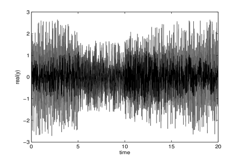
Figure 1: Temporal representation of the simulated data $\mathcal{R}\left[y(t)\right]$ defined by equation(20).

In order to test the robustness of the projection protocol we first compare the original signal $y(t)$ with a reconstructed signal $\tilde{y}(t)$ given by

$$\tilde{y}(t)=\sum_{x_{n}=-175}^{175}c_{x_{n}}^{\theta}(y)\Psi_{x_{n}}^{\theta,T}(t)$$ (22)

The quadratic error $E(y,\tilde{y})$, between the original and the reconstructed signal is less than $-27dB$. The quadratic error is defined as :

$$E(y,\tilde{y})=10\log_{10}\frac{P_{y-\tilde{y}}}{P_{y}}$$ (23)

The quadratic error grows to $-22dB$ if the reconstruction is limited to the range used for the component analysis below (i.e. $45\leq x_{n}\leq{155}$).

The value $\theta=\frac{\pi}{5}$ is chosen by direct inspection of the tomogram of the signal $y(t)$. In this case one sees three well differentiated spectral components (Fig.2). Clearly this is not the unique possible (even logical) choice. From a practical point of view, either some preliminary information is available on the structure of the signal, or we may try different choices of $\theta$ knowing that the incertitude on the time support will increase with $\theta$ whereas the quasi-local frequency incertitude will decrease.

In this example, we performed the factorization of $y(t)$ in three components $\tilde{y_{1}}(t)$, $\tilde{y_{2}}(t)$, and $\tilde{y_{3}}(t)$ defined respectively by the equations (24), (25) and (26) . Using different values of $\theta$, the quadratic errors $E(y,\tilde{y})$, $E(y_{1},\tilde{y_{1}})$, $E(y_{2},\tilde{y_{2}})$ and $E(y_{3},\tilde{y_{3}})$ are computed (Eq. 23). We summarize the corresponding data in the following table:

$\theta$	$\pi$/8	$\pi$/5	3$\pi$/10	4$\pi$/5	$\pi$/2
$E(y_{1},\tilde{y}_{1})$	-14.5dB	-17.5dB	-18.5dB	-17.5dB	-12.5dB
$E(y_{2},\tilde{y}_{2})$	-10.5dB	-12.5dB	-9dB	-7dB	-0.5dB
$E(y_{3},\tilde{y}_{3})$	-14.5dB	-14dB	-13.5dB	-7dB	-4dB
$E(y,\tilde{y})$	-26.5dB	-27dB	-30dB	-30dB	-28dB

In cases where no a priori information is available, different choices of $\theta$ may provide meaningful information about the signal structure. In this example, by looking at the data presented on the table above, the choice of $\theta=\frac{\pi}{5}$ to carry out the factorization seems to give the best performance. Then we simply apply an energy threshold $\epsilon=0.1$, which is about $15\%$ of the energy level of the signal, to decompose the signal $y$ in three components (Fig.2).

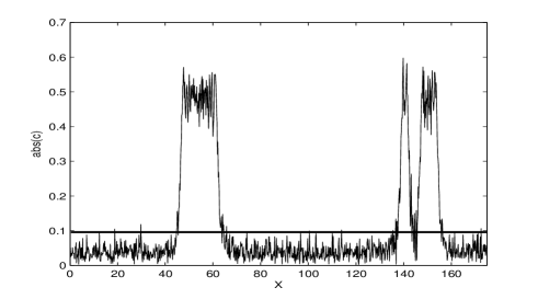
Figure 2: $c_{x_{n}}^{\theta}(y)$ spectrum of the simulated data $y(t)$ for $\theta=\frac{\pi}{5}$ and $0\leq{x_{n}}\leq 175$

The first component, $\tilde{y_{1}}(t)$ corresponds to the spectral range $45\leq x_{n}\leq 65$:

$$\tilde{y_{1}}(t)=\sum_{x_{n}=45}^{65}c_{x_{n}}^{\theta}(y)\Psi_{x_{n}}^{\theta,T}(t)$$ (24)

The second component, $\tilde{y_{2}}(t)$ corresponds to the spectral range $135\leq x_{n}\leq 145$:

$$\tilde{y_{2}}(t)=\sum_{x_{n}=135}^{145}c_{x_{n}}^{\theta_{0}}(y)\Psi_{x_{n}}^{\theta_{0},T}(t)$$ (25)

The real part of $y_{2}(t)$ and $\tilde{y_{2}}(t)$ are presented Fig.3.

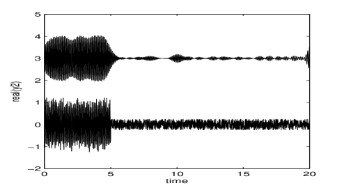
Figure 3: $\mathcal{R}\left[y_{2}(t)\right]$ and $\mathcal{R}\left[\tilde{y_{2}}(t)\right]$. For visual purposes, the mean value of $\mathcal{R}\left[\tilde{y_{2}}(t)\right]$ is shifted to 3.

The last component, $\tilde{y_{3}}(t)$ corresponds to the spectral range $145\leq x_{n}\leq 155$:

$$\tilde{y_{3}}(t)=\sum_{x_{n}=145}^{155}c_{x_{n}}^{\theta}(y)\Psi_{x_{n}}^{\theta,T}(t)$$ (26)

Fig.4 gives a representation of both $\mathcal{R}\left[y_{3}(t)\right]$ and $\mathcal{R}\left[\tilde{y_{3}}(t)\right]$.

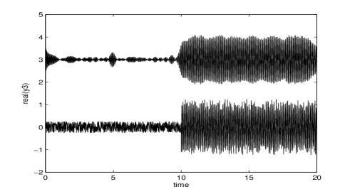
Figure 4: Representation of $\mathcal{R}\left[y_{3}(t)\right]$ and $\mathcal{R}\left[\tilde{y_{3}}(t)\right]$. For visual purposes, the mean value of $\mathcal{R}\left[\tilde{y_{3}}(t)\right]$ is shifted to 3.

The quadratic errors $E(y_{1},\tilde{y_{1}})$, $E(y_{2},\tilde{y_{2}})$ and $E(y_{3},\tilde{y_{3}})$ can be read from the table above. They are, respectively, $-17.5dB$, $-12.5dB$ and $-14dB$.

For comparison, the projection of the simulated data $y(t)$ in the frequency domain ($\theta_{0}=\frac{\pi}{2}$), presented on figure 5, show that the factorization in three components is not possible : only two components can be extract from this projection. At the frequency $x_{n}=25rd/s$, the component will be equal to $\tilde{y_{1}}(t)$. At the frequency $x_{n}=75rd/s$, it will be impossible to set apart $y_{2}(t)$ and $y_{3}(t)$ and the component will be equal to $\tilde{y_{2}}(t)+\tilde{y_{3}}(t)$.

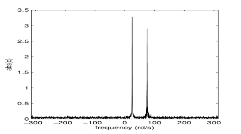
Figure 5: Projection $c^{\theta_{0}}_{x_{n}}$ of the signal for $\theta_{0}=\frac{\pi}{2}$

3.2 Second Example

Here we analyze the decomposition into elementary components of another signal which aims to mimic, in a simplified way, the case of an incident plus a reflected wave delayed in time and with an acquired time-dependent change in phase. In this case the simulated signal $y(t)$ is the sum of an “incident” chirp $y_{0}(t)$ and a “deformed reflected” chirp $y_{R}(t)$. White noise is added to the signal. The incident chirp is:

$$y_{0}(t)=e^{i\Phi_{0}(t)}$$ (27)

with $\Phi_{0}(t)=a_{0}t^{2}+b_{0}t$.

The “instantaneous frequency” of $y_{0}(t)$ sweeps linearly from $75$ $rd/s$ to $50$ $rd/s$ during $20s$. Its phase derivative is linearly dependent on time :$\frac{d}{dt}\Phi_{0}(t)=2a_{0}t+b_{0}$.

The “reflected” signal $y_{R}(t)$ is delayed by $t_{R}=3s$ from the incident one and continuously sweeps from $75rd/s$ to $50rd/s$ :

$$y_{R}(t)=e^{i\Phi_{R}(t)}$$ (28)

where $\Phi_{R}(t)=a_{R}(t-t_{R})^{2}+b_{R}(t-t_{R})+10(t-t_{R})^{\frac{3}{2}}$. In this case the phase derivative $\frac{d}{dt}\Phi_{R}(t)$ is not a linear function. This signal is zero during the first $3s$ seconds and ends up at $t=23s$.

The simulated signal is defined by :

$$y(t)=y_{0}(t)+y_{R}(t)+b(t)$$ (29)

The Signal to Noise Ratio, $SNR(y,b)$, is equal to $15dB$. The real $\mathcal{R}\left[y(t)\right]$ part of this signal is shown in Fig6.

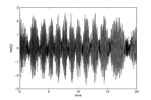
Figure 6: Temporal representation of the simulated data $\mathcal{R}\left[y(t)\right]$ defined by equation(29).

Fig.7 shows $\frac{d}{dt}\Phi_{0}(t)$ and $\frac{d}{dt}\Phi_{R}(t)$ as a function of time. Notice that, except for the three first seconds, the spectrum of the signals $y_{0}(t)$ and $y_{R}(t)$ is almost the same.

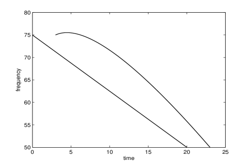
Figure 7: Representation of $\frac{d}{dt}\Phi_{0}(t)$ and $\frac{d}{dt}\Phi_{R}(t)$ as a function of time.

The tomogram of the first $20s$ of $y(t)$, $M_{y}(\theta,x)=\left|<y,\Psi_{x}^{\theta,T}>\right|^{2}$ has a maximum for $\sin(\theta)\approx 0.6$ (Fig.8) corresponding to the “incident” part of the signal that mainly projects in the unique $\Psi_{x}^{\theta,T}$ that matches $\Phi_{0}(t)$. Then, we take the value of $\theta=\pi/5$ to carry out the separation of $y(t)$ in its components.

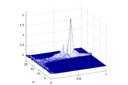
Figure 8: Tomogram of the simulated data defined by Eq.(29)

The corresponding spectrum $c_{x_{n}}^{\theta}(y)$ is shown in Fig.9. Based on this spectrum we decompose the signal in two spectral components.

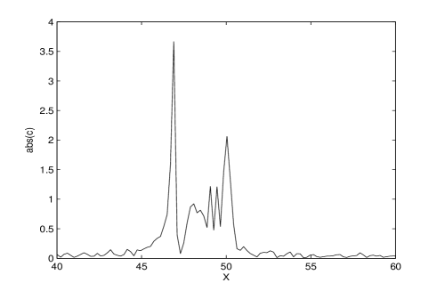
Figure 9: Spectrum of the signal for $\theta=\pi/5$

From the first component we reconstruct the “incident” chirp $y_{0}(t)$ by:

$$\tilde{y_{0}}(t)=\sum_{x_{n}=45}^{47.25}c_{x_{n}}^{\theta_{0}}(y)\Psi_{x_{n}}^{\theta_{0},T}(t)$$ (30)

The quadratic error, between $\tilde{y_{0}}(t)$ and $y_{0}(t)$, $E(y_{0},\tilde{y_{0}})$, is $-9.5dB$.

From the second spectral component we reconstruct the “reflected” chirp given by:

$$\tilde{y_{R}}(t)=\sum_{x_{n}=47.5}^{50.5}c_{x_{n}}^{\theta}(y)\Psi_{x_{n}}^{\theta,T}(t)$$ (31)

In this case the quadratic error $E(y_{R},\tilde{y_{R}})$ is $-10dB$. This may be compared with a quadratic error $E(y,\tilde{y})$ of $-29dB$ for the total signal reconstructed from the spectral projection corresponding to $45<x_{n}<50.5$.

We have tested the method with different delays that encode for the distance of the two “frequencies”. The quality of the disentanglement deteriorates when the delay decreases. But it can still be done for a delay as short as $1s$. Therefore we conclude that the method is quite robust.

4 An application to reflectometry data. Component analysis

We now use signals coming from reflectometry measurement in plasma physics, to show the ability of the tomogram methods to separate different components of the signal to which it is then possible to assign a clear physical meaning. The reflectometry diagnostic is widely used to determine the electronic density profile in a tokamak. The principle, based upon a radar technique [18], is to measure the phase of a probing wave reflected by the plasma cut–off layer at a given density, where the refractive index goes to zero. The determination of the density profile can be achieved by continuously sweeping the frequency of the probing wave.

Different techniques are used to measure the density profile on fusion plasmas [19] (phase difference, ultrashort pulses, continuous sweep, …). A broadband reflectometer operating in the frequency range 50–75 GHz (V band) [20], [21] and 75–110 GHz (W band) [22] has been developed on Tore Supra to measure the electron density profiles at the edge.

The sweep frequency reflectometry system of Tore Supra launches a probing wave on the extraordinary mode polarization (X mode) in the V band (50–75 GHz). The emitting and receiving antennas are located at about 1.20 m from the plasma edge outside the vacuum vessel. The reflectometry system operates in burst mode, i.e. the sweeps are performed repeatedly every $25\mu s$. The duration of one sweep, $E_{0}(t)=A_{0}e^{i\phi(t)}$, is $20\mu s$ and 5000 chirps are send during one measurement. During the $20\mu s$ measurement time, the frequency of the probing wave is continuously sweeping, from 50 GHz to 75 GHz (V band).

The heterodyne reflectometers, with I/Q detection, provide a good Signal to Noise Ratio, up to $40dB$. For each sweep, the reflected chirp $E_{R}(t)$ is mixed with the incident sweep $E_{0}(t)$ and only the interference term is recorded as in-phase and $90^{\circ}$ phase shifted signals sampled at $T_{e}=10^{-8}s$

$$x_{1}(t)=A_{0}A_{R}(t)\cos(\varphi(t))$$

$$x_{2}(t)=A_{0}A_{R}(t)\sin(\varphi(t))$$

For each sweep, the phase $\varphi(t)$ of the reflected signal is represented by

$$y(t)=x_{1}(t)+ix_{2}(t)=A(t)e^{i\varphi(t)}$$ (32)

The amplitude of this signal $A(t)=A_{0}A_{R}(t)$ is low frequency. The real part of one such signal $y(t)$ is shown in Fig.10.

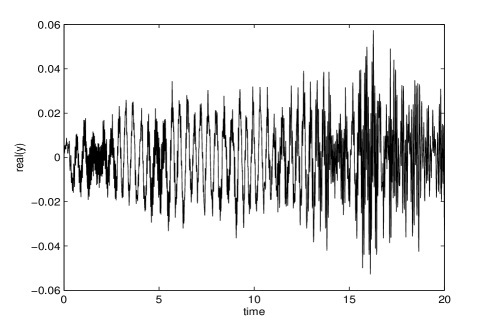
Figure 10: Time representation of the reflectometry signal.

The tomogram $M_{y}(x,\theta)$ of the signal is shown in Fig.11 where it is possible to see that it carries three main different components.

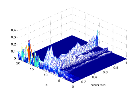
Figure 11: Tomogram of the reflectometry signal.

The choice of $\theta=\frac{3\pi}{10}$ to perform the factorization of the signal was done by simple inspection of this tomogram. The spectrum $c_{x_{n}}^{\theta}(y)$ of the reflectometry signal for $\theta=\frac{3\pi}{10}$ is shown in Fig.12.

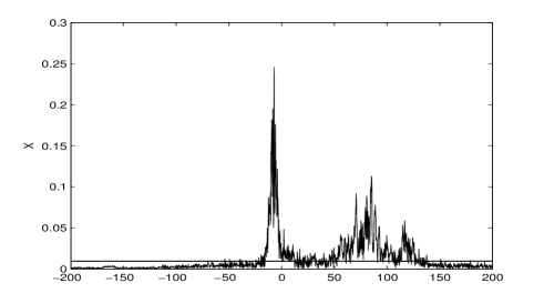
Figure 12: Spectrum $c^{\theta}_{x_{n}}$ of the reflectometry signal $y(t)$ for $\theta=\frac{3\pi}{10}$

When reconstructing $\tilde{y}(t)$ by:

$$\tilde{y}(t)=\sum_{x_{n}=-200}^{200}c_{x_{n}}^{\theta}(y)\Psi_{x_{n}}^{\theta,T}(t)$$ (33)

the quadratic error $E(y,\tilde{y})$, between the original and the reconstructed signals is $-25dB$.

Factorization of the reflectometry signal

By taking a threshold equal to $\epsilon=0.01$ we select the spectral components corresponding to $\left|c_{x_{n}}\right|\neq 0$ for $-20\leq x_{n}\leq 140$ (see Fig.13). The error between the original and the selected signal is about $-18dB$. From there the spectrum of $y(t)$ splits in three components.

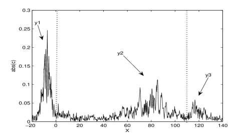
Figure 13: Part of the spectrum $c^{\theta}_{x_{n}}(y)$ of the reflectometry signal used in the factorization

First component, the reflection on the porthole

The first component, $\tilde{y_{1}}(t)$ corresponds to $-20\leq x_{n}\leq 0$ and is therefore defined as:

$$\tilde{y_{1}}(t)=\sum_{x_{n}=-20}^{0}c_{x_{n}}^{\theta}(y)\Psi_{x_{n}}^{\theta}(t)$$ (34)

It is a low frequency signal corresponding to the heterodyne product of the probe signal with the reflection on the porthole [22]. It is shown in Fig.14.

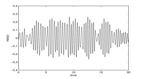
Figure 14: First component of the reflectometry signal corresponding to the reflection on the porthole

Second component, the plasma signal

The second component has a Fourier spectra that fits the expected behavior corresponding to the reflection of the wave inside the plasma of the tokamak, [22]. This component, $\tilde{y_{2}}(t)$, corresponds to $0\leq x_{n}\leq 110$ and is therefore defined as:

$$\tilde{y_{2}}(t)=\sum_{x_{n}=0}^{110}c_{x_{n}}^{\theta}(y)\Psi_{x_{n}}^{\theta}(t)$$ (35)

It is shown in Fig.15.

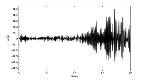
Figure 15: Second component of the reflectometry signal, corresponding to the reflection on the plasma

Third component, the multi-reflection component

The last component corresponds [22] to multi reflections of the waves on the wall of the vacuum vessel. This component, $\tilde{y_{3}}(t)$, corresponds to $110\leq x_{n}\leq 140$ and is therefore defined as:

$$\tilde{y_{3}}(t)=\sum_{x_{n}=10}^{140}c_{x_{n}}^{\theta}(y)\Psi_{x_{n}}^{\theta}(t)$$ (36)

This component is shown in Fig.16.

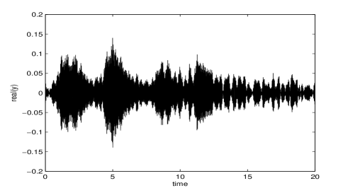
Figure 16: Third component of the reflectometry signal, corresponding to multi reflections on the vessel

We notice that by undertaking a new factorization of this third component it seems possible to separate different successive reflections of the wave but this would be out of the scope of this work.

The three components of the reflectometry signal are presented together on the same plot (Fig. 17). It is instructive to compare this factorization with the original reflectometry signal (see Fig. 10).

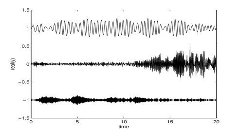
Figure 17: The three components of the reflectometry signal. For visual purposes, the average of $\tilde{y_{1}}(t)$ is shifted to 1 and the average of $\tilde{y_{3}}(t)$ to -1.

5 Remarks and conclusions

1) Based on a complete and probabilistically rigorous spectral analysis and projection on the eigenvectors of a family of unitary operators, our method seems quite robust to disentangle the relevant components of the signals. This has been demonstrated both on simulated and on experimental reflectometry data. In particular in this last case, a clear identification of the physical origin of the components and its separation is readily achieved. Such separation could not be achieved by the simple filtering techniques. After the component separation phase, the method also provides by truncation of some subsets of the projection coefficients a very flexible denoising technique.

Another important conclusion from this study is the fact that by the choice of different families of (unitary) operators and their spectral representations, different traits and components of the signals may be emphasized.

2) In the analysis of reflectometry data, component separation and denoising is a required first step to obtain reliable information on the plasma density. In particular, accuracy in these measurements is quite critical if in addition to the average local density one also wants to have information on plasma fluctuations and turbulence.

The location $x_{c}\left(\omega_{p}\right)$ of the reflecting (cut-off) layer for the frequency $\omega_{p}$ is related to the group delay[23] [24] :

$$\tau_{g}=\frac{d\phi\left(\omega\right)}{d\omega}=\frac{1}{2\pi}\frac{d\phi}{df}$$ (37)

and for a linear frequency sweep of the incident wave

$$f\left(t\right)=f_{0}+\gamma t$$ (38)

one obtains

$$\frac{d\phi}{df}=\frac{1}{\gamma}\left.\frac{d\phi}{dt}\right|_{f}$$ (39)

Therefore, measurement of the plasma density hinges on an accurate determination of the “instantaneous frequency” $\frac{d\phi}{dt}$. Accuracy in the measurement of this quantity is quite critical because, the location of the reflecting layer being obtained from an integral, errors tend to accumulate.

Several methods have been devised to obtain the group delay $\tau_{g}$ from the reflectometry data (for a review see [24]). Among them, time-frequency analysis[25] was widely explored. The Wigner-Ville (WV) distribution [26] [27], although providing a complete description of the signal in the time-frequency plane, raises difficult interpretation problems due to the presence of many interference terms that impair the readability of the distribution. For this reason the time-frequency method that, so far, has been preferred is the spectrogram[25] [28] [29], that is, the squared modulus of the short-time Fourier transform

$$SP\left(t,f\right)=\left|\int_{-\infty}^{\infty}x\left(u\right)h\left(u-t\right)e^{-i2\pi fu}du\right|^{2}$$

$h\left(u\right)$ being a peaked short-time window.

The spectrogram does not really provide the instantaneous frequency, because that notion is not well defined anyway. All it gives is the product of the spectra of $x\left(t\right)$ and $h\left(t\right)$. The way the spectrogram is used to infer the local rate of phase variation $\frac{d\phi}{dt}$ is to identify this quantity with the maximum or the with the first moment of the spectrogram. An additional problem comes about because unwanted phase contributions due to plasma turbulence may have a higher amplitude than the contributions due to the profile. Correction techniques have been developed to compensate for this errors, based for example on Floyd’s best path algorithm. The choice of the window function is also an important issue and, in particular, an adaptive spectrogram technique has been developed to maximize the time-frequency concentration[24].

Here, the tomographic method may also provide a needed improvement, namely by obtaining the phase derivative directly from the coefficients $c_{n}$ of the plasma reflection component. This, together with the selective denoising techniques after component separation, will be described in a forthcoming paper.

6 Appendix A. Gauss-Hermite decomposition of the tomograms

From the definition (10) of the tomogram transform one sees that the calculation from the data near $\nu=0$ has accuracy problems because of the fast variation of the phase in (10). Two techniques are used to deal with this problem. The first one uses a projection of the time signal $s\left(t\right)$ on an orthogonal basis and the second uses the homogeneity properties (11) and an expansion of the Fresnel tomogram near $\nu=0$. The first technique is described in this appendix and the second in the Appendix B.

Let $s\left(t\right)$ be a normalized signal

$$\int|s(t)|^{2}dt=1.$$ (40)

Decompose the signal in Gauss-Hermite polynomials

$$s(t)=\sum_{n=0}^{\infty}c_{n}(t)\psi_{n}(t),$$ (41)

with

$$\psi_{n}(t)=\frac{e^{-t^{2}/2}}{\pi^{1/4}}\,\frac{1}{\sqrt{2^{n}n!}}\,H_{n}(t).$$ (42)

and

$$c_{n}=\int s(t)\psi_{n}(t)\,dt,$$ (43)

Then, the tomogram of the signal is

$$M_{s}(X,\mu,\nu)=M_{0}(X,\mu,\nu)\left|\sum_{n=0}^{\infty}c_{n}\frac{1}{\sqrt{n!}}\left(\frac{1}{2}-\frac{1}{1-i\mu/\nu}\right)^{n/2}H_{n}\left(\frac{b}{2\sqrt{k}}\right)\right|^{2},$$ (44)

with

$$M_{0}(X,\mu,\nu)=\frac{1}{\sqrt{\pi\left(\mu^{2}+\nu^{2}\right)}}\,e^{-X^{2}/\left(\mu^{2}+\nu^{2}\right)}$$ (45)

and

$$b=\frac{i\sqrt{2}X}{i\mu-\nu},\qquad k=\left(\frac{1}{2}-\frac{1}{1-i\mu/\nu}\right).$$ (46)

7 Appendix B. The Fresnel tomogram

The symplectic tomogram $M_{s}(X,\mu,\nu)$ can be reconstructed if one knows the (Fresnel) tomogram  [30]

$$M_{\mathrm{F}}(X,\nu)=M_{s}(X,1,\nu)$$ (47)

due to the homogeneity property (11). In fact, one has

$$M_{s}(X,\mu,\nu)=\frac{1}{|\mu|}\,M_{s}\left(\frac{X}{\mu}\,,1,\frac{\nu}{\mu}\right)$$ (48)

which means that, if one knows $M_{\mathrm{F}}(\widetilde{X},\widetilde{\nu})$, the symplectic tomogram is obtained by replacement and a factor,

$$M_{s}(X,\mu,\nu)=\frac{1}{|\mu|}\,M_{\mathrm{F}}\left(\widetilde{X}\rightarrow\frac{X}{\mu}\,,\widetilde{\nu}\rightarrow\frac{\nu}{\mu}\right)$$ (49)

In terms of signal $s(t)$ it reads:

$$M_{\mathrm{F}}(X,\nu) = \frac{1}{2\pi|\nu|}\left|\int e^{i(X-y)^{2}/2\nu}s(y)\,dy\right|^{2}$$ (50)

$$= \left|\int\frac{1}{\sqrt{2\pi|\nu|}}e^{i(X-y)^{2}/2\nu}s(y)\,dy\right|^{2}$$

$$= \left|\exp\left[-i\nu\left(-\frac{1}{2}\,\frac{\partial^{2}}{\partial X^{2}}\right)\right]s(X)\right|^{2}$$

Thus for small $\nu$ one has

$$M_{s}(X,\mu,\nu)\approx\frac{1}{|\mu|}\left|s\left(\frac{X}{\mu}\right)-\frac{i\nu}{2}\,s^{\prime\prime}\left(\frac{X}{\mu}\right)\right|^{2}.$$ (51)

In the Gauss-Hermite basis it is

$$M_{\mathrm{F}}(X,\nu)=\frac{e^{-X^{2}/(1+\nu^{2})}}{\sqrt{\pi(1+\nu^{2})}}\left|\sum_{n=0}^{\infty}c_{n}\,\frac{1}{\sqrt{n!}}\left(\frac{1}{2}-\frac{1}{1-i/\nu}\right)^{n/2}H_{n}\left(\frac{\tilde{b}}{2\sqrt{\tilde{k}}}\right)\right|^{2},$$ (52)

with

$$\tilde{b}=\frac{i\sqrt{2}X}{i-\nu},\qquad\tilde{k}=\left(\frac{1}{2}-\frac{1}{1-i/\nu}\right).$$ (53)

As a series, the Fresnel tomogram is

$$M_{F}(X,\nu)\approx\left|\sum_{k=0}^{\infty}\left(\frac{i\nu}{2}\right)^{k}\,\frac{1}{k!}\,\frac{d^{2k}f(X)}{dX^{2k}}\right|^{2},$$ (54)

leading to a symplectic tomogram

$$M(X,\mu,\nu)=\frac{1}{|\mu|}\left|\sum_{k=0}^{\infty}\left(\frac{i\nu}{2\mu}\right)^{k}\,\frac{1}{k!}\frac{d^{2k}f(X/\mu)}{dX^{2k}}\right|^{2}.$$ (55)

Since

$$-\frac{1}{2}\,\frac{\partial^{2}}{\partial t^{2}}\,s_{n}(t)+\frac{t^{2}}{2}\,s_{n}(t)=\left(n+\frac{1}{2}\right)s_{n}(t),\qquad n=0,1,2,\ldots,$$ (56)

on has, for small $\nu$, the following Fresnel tomogram of $s_{n}(t)$:

$$M_{n}(X,\mu=1,\nu)\approx s_{n}^{2}(X)\left[1+\left(n+\frac{1}{2}-\frac{X^{2}}{2}\right)\nu^{2}\right]$$ (57)

Acknowledgements

V.I.Man’ko thanks ISEG - Lisbon (Instituto Superior de Economia e Gest$\tilde{a}$o) for kind hospitality.

References

- [1] L. Cohen; Time-frequency distributions - A review, Proc. IEEE 77 (1989) 941-981.
- [2] L. Cohen; What is a multi-component signal?, IEEE Proc. Int. Conf. Acoust. Speech Signal Process. ’92, vol.5, pp.113-116, 1992.
- [3] L. M. Khadra; Time-frequency distribution of multi-component signals, Int. J. of Electronics 67 (1989) 53-57.
- [4] H. I. Choi and W. J. Williams; Improved time-frequency representaion of multi-component signals using exponential kernels, IEEE Trans. Acoust. Speech Signal Process. 37 (1989) 862-871.
- [5] A. B. Fineberg and R. J. Mammone; Detection and classification of multicomponent signals, in Proceedings of 25th Asilomar Conference on Computer, Signal and Systems, pp. 1093-1097, 1991.
- [6] G. Jones and B. Boashash; Instantaneous frequency, instantaneous bandwidth and the analysis of multicomponent signals, Int. Conf. on Acoustics, Speech and Signal Process. ICASSP90, pp. 2467-2470, 1990.
- [7] A. Francos and M. Porat; Analysis and synthesis of multicomponent signals using positive time-frequency distributions, IEEE Trans. on Signal Process. 47 (1999) 493-504.
- [8] P. Flandrin; Localisation dans le Plan Temps-Fréquence, Traitement du Signal 15 (1999) 483-492.
- [9] B. Boashash; Estimating and interpreting the instantaneous frequency of a signal (parts 1 and 2), Proc. IEEE 80 (1992) 520-538 and 540-568.
- [10] H. Rong, G. Zhang and W. Jin; Application of S_method to multi-component emitter signals, Proc. 33th. Annual Conf. of the IEEE Ind. Electronics Soc. , pp. 2521-2525, 2007
- [11] Y. Wang and Y. Jiang; Generalized time-frequency distributions for multicomponent polynomial phase signals, Signal Processing 88 (2008) 984-1001.
- [12] M. A. Man’ko, V. I. Man’ko and R. Vilela Mendes; Tomograms and other transforms: a unified view, J. Phys. A: Math. Gen. 34 (2001) 8321-8332.
- [13] V. I. Man’ko and R. Vilela Mendes; Noncommutative time–frequency tomography, Phys. Lett. A 263 (1999) 53–59.
- [14] I. M. Gel’fand, M. I. Graev and N. Y. Vilenkin; Generalized Functions, Integral Geometry and Representation Theory , vol.5, Academic Press, New York, 1966.
- [15] J. Wood and D. T. Barry; Linear signal synthesis using the Radon-Wigner transform, IEEE Trans. on Signal Process. 42 (1994) 2105-2111.
- [16] J. Wood and D. T. Barry; Radon transformation of time-frequency distributions for analysis of multicomponent signals, IEEE Trans. on Signal Process. 42 (1994) 3166-3177.
- [17] S. Barbarossa; Analysis of multicomponent LFM signals by a combined Wigner-Hough transform, IEEE Trans. on Signal Process. 43 (1995) 1511-1515.
- [18] C. A. Hugenholtz and S. H. Heijnen; Pulse radar technique for reflectometry on thermonuclear plasmas, Rev. Sci. Instrum. 62 (1991) 1100-1101
- [19] C. Laviron, A. J. H. Donné, M. E. Manso and J. Sanchez; Reflectometry techniques for density profiles measurements on fusion plasmas, Plasma Phys. Control. Fusion 38 (1996) 905-936
- [20] F. Clairet, C. Bottereau, J. M. Chareau, M. Paume and R. Sabot; Edge density profile measurements by X-mode reflectometry on Tore Supra, Plasma Phys. Control. Fusion 43 (2001) 429-442
- [21] F. Clairet, R. Sabot, C. Bottereau, J. M. Chareau, M. Paume, S. Heureaux, M. Colin, S. Hacquin and G. Leclert; X-mode heterodyne reflectometer for edge density profile measurements on Tore Supra, Rev. Sci. Instrum. 72 (2001) 340-343
- [22] F. Clairet, C. Bottereau, J. M. Chareau and R. Sabot; Advances of the density profile reflectometry on TORE SUPRA, Rev. Sci. Instrum. 74 (2003) 1481-1484
- [23] F. Simonet; Measurement of electron density profile by microwave reflectometry on tokamaks, Rev. Sci. Instrum. 56 (1985) 664-669.
- [24] P. Varela, M. E. Manso and A. Silva; Review of data processing techniques for density profile evaluation from broadband FM-CW reflectometry on ASDEX Upgrade, Nuclear Fusion 46 (2006) S693-S707.
- [25] P. Varela, M. E. Manso, I. Nunes, A. Silva and F. Silva; Automatic evaluation of plasma density profiles from microwave reflectometry on ASDEX upgrade based on the time-frequency distribution of the reflected signals, Review of SCi. Instrum. 70 (1999) 1060-1063.
- [26] F. Nunes, M. E. Manso, I. Nunes, J. Santos, A. Silva and P. Varela; On the application of the Wigner-Ville distribution to broadband reflectometry, Fusion Engineering and Design 43 (1999) 441-449.
- [27] J. P. S. Bizarro and A. C. Figueiredo; The Wigner distribution as a tool for time-frequency analysis of fusion plasma signals: application to broadband reflectometry signals, Nuclear Fusion 39 (1999) 61-82.
- [28] F. Clairet, R. Sabot, Ch. Bottereau, J. M. Chareau and M. Paume; X-mode heterodyne reflectometer for edge density profile measurements on Tore Supra, Review of Sci. Instrum. 72 (2001) 340-343.
- [29] F. Silva, M. E. Manso, P. Varela and S. Hereaux; A 2d fdtd full-wave code for simulating the diagnostic of fusion plasmas with microwave reflectometry, Proc. Computational Methods in Engineering and Science (Macau, China) pp 955-961.
- [30] De Nicola, R.Fedele ,M.A.Manko and V.I.Manko ;Fresnel Tomography: A Novel Approach to Wave-Function Reconstruction Based on the Fresnel Representation of Tomograms Theor.Math.Phys.,v.144,pp.1206-1213(2005)