Time-dependent natural orbitals and occupation numbers

Abstract

We report equations of motion for the occupation numbers of natural spin orbitals and show that adiabatic extensions of common functionals employed in ground-state reduced-density-matrix-functional theory have the shortcoming of leading always to occupation numbers which are independent of time. We illustrate the exact time-dependence of the natural spin orbitals and occupation numbers for the case of electron-ion scattering and for atoms in strong laser fields. In the latter case, we observe strong variations of the occupation numbers in time.

The description of quantum many-body systems out of equilibrium has become an important research topic in nuclear, plasma and condensed-matter physics. The common interest of different fields in non-equilibrium quantum evolution is mainly driven by experimental and technological progress which raises questions such as how many-body systems evolve on transient or non-adiabatic time-scales, how they thermalize or which kind of transport phenomena are to be expected in extreme environments.

The Kadanoff-Baym equations KB62 ; D84 ; B98 provide a rigorous basis to investigate the dynamics of non-equilibrium many-body systems. Although the equations are known for some decades, so far only ab-initio solutions for very small atomic or molecular systems under special assumptions have been achieved DL07 ; TR08 . For a more comprehensive ab-initio treatment of non-equilibrium systems with many degrees of freedom they are still out of scope of present day computing facilities.

An alternative for the study of non-equilibrium processes in many-body systems is provided by time-dependent density-functional theory (TDDFT) MUN06 . TDDFT is currently the method of choice for electronic systems out of equilibrium because it generally achieves decent accuracy at affordable computational cost. All physical observables are in principle functionals of the time-dependent density RG84 ; L99 . However, in practice it is sometimes rather cumbersome to find approximate expressions for observables of interest. Prominent examples are double and above-threshold ionization of atoms and molecules in strong laser fields, where no accurate functionals for the observables are known LL98 .

Recently, there has been renewed interest in reduced-density-matrix-functional theory (RDMFT) GU98 ; BB02 . RDMFT is a promising candidate to treat long standing problems present in traditional density-functional theory (DFT). RDMFT describes very accurately the cohesion and dissociation of diatomic molecules which presents a difficult problem for DFT methods due to the importance of static correlation GPB05 . The theory has also been successfully applied to the calculation of the fundamental gap HLA05 .

In this work we consider the description of non-equilibrium many-particle systems in terms of time-dependent reduced-density matrices. These density matrices have the potential to capture the physics of strong correlations SDLG08 in the time-dependent case and, furthermore, observables can be more easily extracted from density matrices than from the density alone.

The time-evolution of the reduced density matrices is given by the Bogoliubov-Born-Green-Kirkwood-Yvon (BBGKY) hierarchy of equations of motion B61 . The first equation of the hierarchy has the form

$$\begin{split}i\partial_{t}\gamma_{1}(&11^{\prime};t)=\left(\hat{h}_{0}(1;t)-\hat{h}_{0}(1^{\prime};t)\right)\gamma_{1}(11^{\prime};t)\\ &+\int\left(v_{\rm ee}(12)-v_{\rm ee}(1^{\prime}2)\right)\gamma_{2}(121^{\prime}2^{\prime};t)|_{2^{\prime}=2}\,d2,\end{split}$$ (1)

where the bare single particle Hamiltonian is given by $\hat{h}_{0}(1;t)=-\nabla^{2}_{1}/2+v_{\rm ext}(1)$ and $v_{\rm ee}(12)$ denotes the particle-particle interaction. The coordinates are written as combined space-spin variables $1=({\bf r}_{1},\sigma_{1})$ and we use $\int d1=\sum_{\sigma_{1}}\int d{\bf r}_{1}$. In general, similar equations in the BBGKY hierarchy connect the time-evolution of the N-th order reduced density matrix $\gamma_{N}$ to the density matrix of order N+1. Since $2N$ cordinates appear in the equation of order N, the propagation of the complete hierarchy is even more involved than solving the underlying time-dependent Schrödinger equation (TDSE). Hence, truncations of the hierarchy are performed in practice. To close the system of evolution equations at a given order N it is therefore necessary to express the matrix of order N+1 in terms of matrices with order less or equal to N. This is the central point where approximations enter in a time-dependent reduced density matrix theory. Note, that in the case of two-body interactions $v_{\rm ee}(12)$ it is sufficient for the calculation of the ground-state energy to know the diagonal of the two-body reduced density matrix $\gamma_{2}(1212;t=0)$. As can be seen directly from Eq. (1), this is in contrast to the time-dependent case, where also off-diagonal matrix elements $\gamma_{2}(121^{\prime}2;t\geq 0)$ enter the equation of motion.

By diagonalizing the one-body reduced-density matrix $\gamma_{1}(11^{\prime};t)$ at each fixed point in time one obtains eigenvectors $\varphi_{j}(1;t)$ and eigenvalues $n_{j}(t)$ which we term, in analogy to static RDMFT, time-dependent natural orbitals and time-dependent occupation numbers, respectively PGB07 . The spectral representation of the one-body matrix then takes the form

$$\gamma_{1}(11^{\prime};t)=\sum_{k}n_{k}(t)\varphi_{k}(1;t)\varphi^{*}_{k}(1^{\prime};t).$$ (2)

Since the eigenvectors $\varphi_{j}(1;t)$ form a complete set at each point in time, we can also express the two-body reduced matrix in the basis of natural orbitals of the one-body matrix

$$\gamma_{2}(12,1^{\prime}2^{\prime};t) = \sum_{ijkl}\gamma_{2,ijkl}(t)\times$$

$$\varphi_{i}(1;t)\varphi_{j}(2;t)\varphi^{*}_{k}(1^{\prime};t)\varphi^{*}_{l}(2^{\prime};t).$$

With Eq. (2) the time-dependent natural orbitals and occupation numbers have been introduced by a diagonalization procedure. It is now interesting to observe that the occupation numbers obey evolution equations which have the following form

$$i\,\dot{n}_{k}(t)=\sum_{ijl}\gamma_{2,ijkl}(t){\langle\,}ij\,|\,v_{\rm ee}\,|\,kl{\,\rangle}(t)-c.c.$$ (4)

where we have used ${\langle\,}ij\,|\,v_{\rm ee}\,|\,kl{\,\rangle}(t)$ as shorthand for the coulomb integrals

$$\int\varphi_{i}(1;t)\varphi_{j}(2;t)v_{\rm ee}(12)\varphi^{*}_{k}(1;t)\varphi^{*}_{l}(2;t)\,d1d2.$$ (5)

Next, we separate the coefficients $\gamma_{2,ijkl}(t)$ into a mean-field and a cummulant part $\lambda_{2,ijkl}(t)$ KM99

$$\gamma_{2,ijkl}(t)=n_{i}(t)n_{j}(t)(\delta_{ik}\delta_{jl}-\delta_{il}\delta_{jk})+\lambda_{2,ijkl}(t).$$ (6)

Inserting (6) into the equation of motion for the occupation numbers (4) one finds, that Hartree and exchange-like contributions cancel. Consequently, we obtain that only the remaining cumulant part of the two-body reduced density matrix determines the time-evolution of the occupation numbers

$$i\,\dot{n}_{k}(t) = \sum_{ijl}\lambda_{2,ijkl}(t){\langle\,}ij\,|\,v_{\rm ee}\,|\,kl{\,\rangle}(t)-c.c.$$ (7)

For the closure of the BBGKY hierarchy up to level N=1 an approximation of the two-body reduced density matrix in terms of the one-body matrix is required. One might be tempted to extend common functionals used in static RDMFT to the time-dependent case in a spirit similar to the adiabatic local density approximation of TDDFT TGK08 , i.e. for a slowly varying time-dependence in the Hamiltonian the ground-state functional is evaluated at the time-dependent density. In the case of time-dependent reduced density matrices this corresponds to replacing the ground-state occupation numbers by their time-dependent counterparts. Although this replacement is rather ad hoc, the hope would be that such functionals perform also reasonably well in non-adiabatic situations.

The functional form of most commonly used ground-state functionals in RDMFT, written in the basis of the natural orbitals, can be summarized with the following expression

$$\gamma_{2,ijkl}=f_{ijkl}\delta_{ik}\delta_{jl}-g_{ijkl}\delta_{il}\delta_{jk},$$ (8)

which contains Hartree ($\delta_{ik}\delta_{jl}$) and exchange-like ($\delta_{il}\delta_{jk}$) terms. As example, for the Müller functional M84 we have $f_{ijkl}=1/2\,n_{i}\,n_{j}$, $g_{ijkl}=1/2\,\sqrt{n_{i}\,n_{j}}$, the self-interaction corrected functional of Goedecker and Umrigar GU98 reads $f_{ijkl}=1/2\,(n_{i}\,n_{j}-n^{2}_{i}\delta_{ij}\delta_{ik}\delta_{il})$, $g_{ijkl}=1/2\,(\sqrt{n_{i}\,n_{j}}-n_{i}\delta_{ij}\delta_{ik}\delta_{il})$ and the BBC1 functional of Baerends et al. GPB05 has the form $f_{ijkl}=1/2\,n_{i}\,n_{j}$, $g_{ijkl}=\sqrt{n_{i}\,n_{j}}(1/2\,-\delta_{il}\delta_{jk}(1-\delta_{ij})\Theta(i-N-\epsilon)\Theta(j-N-\epsilon))$, where $\Theta$ denotes the usual Heaviside step function and $0<\epsilon<1$. In a similar fashion the BBC2/BBC3 functionals can be written in the form of Eq. (8). Note, that all functionals have the symmetry $g_{ijkl}=g_{jilk}$ and all matrices $f_{ijkl}$, $g_{ijkl}$ are real valued.

Replacing the static occupation numbers which appear in Eq. (8) by their time-dependent counterparts and inserting this approximation for the two-body matrix into the equation of motion for the occupation numbers (4) we obtain

$$\begin{split}i\,\dot{n}_{k}(t)&=\sum_{j}(f_{kjjk}(t)-f^{*}_{kjjk}(t)){\langle\,}kj\,|\,v_{\rm ee}\,|\,kj{\,\rangle}(t)\\ &\>+\sum_{j}(g^{*}_{jkkj}(t)-g_{jkkj}(t)){\langle\,}jk\,|\,v_{\rm ee}\,|\,kj{\,\rangle}(t),\end{split}$$ (9)

which shows that all functionals of the form (8) with real valued matrices $f_{ijkl}$, $g_{ijkl}$ cause a zero right hand side in (9). Hence, if this class of approximations is used for the time-evolution of the one-body matrix $\gamma_{1}$, the occupation numbers stay constant in time. This is a severe shortcoming of an adiabatic extension of present functionals of static RDMFT which needs to be addressed in the development of future functionals. Possible functional forms that lead to a non-vanishing right hand side in (9) would be $\gamma_{2,ijkl}(t)=g(f_{ik}(t)\,f_{jl}(t)-f_{il}(t)\,f_{jk}(t))$ or $\gamma_{2,ijkl}(t)=g((f_{ij}(t)-f_{ji}(t))(f_{kl}(t)-f_{lk}(t)))$, where $f_{ij}$ is a non-diagonal real-valued matrix and $g$ some Taylor-expandable function. Alternatively, functionals with complex valued matrices could be employed.

Figure 1: (a) Correlation entropy of e-He⁺ scattering for different interaction strengths $\lambda$. (b), (c) Occupation numbers for the largest natural orbitals, respectively.

How do occupation numbers actually change in time? In the discussion above we have seen that present functionals of static RDMFT would lead to time-independent occupation numbers. Is this a sensible approximation? To date the time-dependence of occupation numbers and natural orbitals is totally unknown. Take as an example the He atom and consider a transition from the ground state (where the two 1s natural spin orbitals have occupation numbers close to $1$) to the first excited state (where the 1s and the 2p spin orbitals have spin-degenerate occupation numbers close to 1/2) by virtue of an optimized laser pulse. How do occupation numbers and natural orbitals evolve during the transition? At first sight two extreme scenarios are conceivable for this case: (i) the occupation numbers stay nearly constant in time and only the orbitals change as follows: 1s $\to$ 1s, 1s $\to$ 2p; or the opposite scenario: (ii) the orbitals stay close to the initial orbitals and only the occupation numbers change to achieve the (1s,2p) final state. Particularly interesting is the fact that this is a transition from a weakly correlated to a strongly correlated state (the latter being a superposition of two determinants).

To investigate the exact time-dependence of natural orbitals and occupation numbers we consider two prototypical cases: (i) e-He⁺ scattering and (ii) the above mentioned transition of the Helium atom from the ground state to the first excited state induced by an optimized short laser pulse. In both cases we limit ourselves to reduced dimensionality so that the full time-dependent many-body Schrödinger equation can be solved numerically. From the exact time-dependent many-body wave function we compute the one-body reduced density matrix and by diagonalizing the matrix at each point in time we obtain the natural orbitals and occupation numbers. We evolve both systems (i) and (ii) under a Soft-Coulomb Hamiltonian SE91 of the form

$$\hat{H}_{\lambda} = \frac{\hat{p}_{1}^{2}}{2}+\frac{\hat{p}_{2}^{2}}{2}\,-\,\frac{2}{\sqrt{\hat{x}_{1}^{2}+1}}\,-\,\frac{2}{\sqrt{\hat{x}_{2}^{2}+1}}$$

$$\,+\,\frac{\lambda}{\sqrt{(\hat{x}_{1}-\hat{x}_{2})^{2}+1}}.$$

To vary the degree of correlation in the many-body wave function we introduce a coupling constant $\lambda$ in the Hamiltonian which controls the strength of the electron-electron interaction.

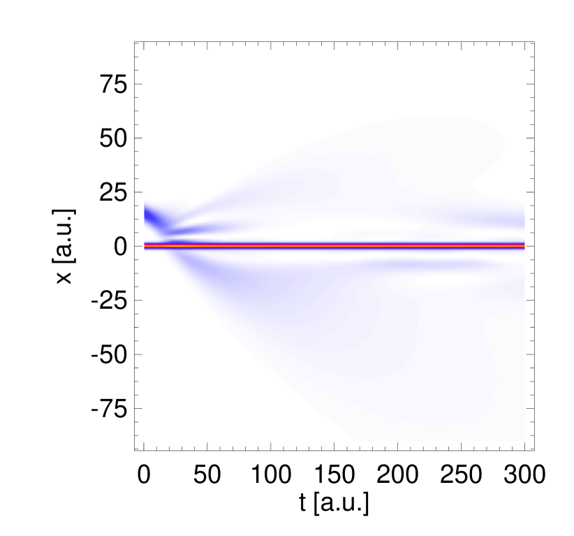
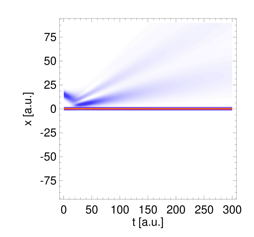
Figure 2: Space-time plot of the electron density for e^- – He⁺ scattering. (a) $\lambda=1.0$, (b) $\lambda=2.0$.

Ref. Z00 introduced the correlation entropy

$$s(\{n_{k}\}):=-\frac{1}{N}\,Tr\gamma_{1}\ln\gamma_{1}=-\frac{1}{N}\,\sum_{k}n_{k}\ln n_{k}$$ (11)

as a measure for the correlation which is contained in the one-body reduced density matrix. The correlation entropy $s$ defined in this way is identical to zero for noninteracting particles and grows with increasing correlation in the system. In our time-propagations we calculate $s(\{n_{k}(t)\})$ as function of time to monitor the degree of correlation which is present in the many-body wave function at a given instant in time.

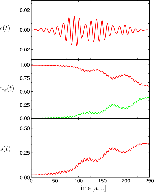
Figure 3: (a) Optimal laser pulse for the transition of the Helium atom from the ground state to the first excited singlet state. The overlap of the propagated wave-function and the target state was 98.59% after 12 OCT iterations. (b) The two largest occupation numbers and (c) the correlation entropy as function of time.

Case (i) - electron-ion scattering. For the initial state of the propagation we consider an antisymmetric spin singlet product wave function formed from a Gaussian wave packet $\psi(x)=\exp(-(x-x_{0})^{2}/\sigma^{2})\exp(-k_{0}x)$ and the ground state $\phi_{0}(x)$ of the He⁺-ion. For all calculations we place the packet initially at a distance of $x_{0}=15$ a.u. away from the ionic core and give the scattering electron a momentum of $k_{0}=0.3$ a.u. which is pointing towards the ion. In Fig. 1 we plot the occupation numbers and the correlation entropy as function of time for different values of the electron-electron interaction strength $\lambda$. After about $t=10$ a.u. the wave packet has approached the ionic core and is passing the atomic nucleus. During this time the degree of correlation in the wave function is enhanced. After the collision the transmitted and reflected waves are leaving the ionic center (cf. Fig. 2) and the correlation entropy starts to decrease. As indicated by the correlation entropy for long times after the scattering event, the many-body wave-function is again well represented by a single Slater determinant. The occupation numbers deviate most strongly from their determinantal values (0 or 1) for $\lambda=1.5$. For $\lambda=2.0$ the electron-electron repulsion is already so strong that the incident wave packet is mainly reflected back.

Case(ii) - optimal control. To study laser induced transitions in the Helium atom we add an external dipole laser field of the form $\hat{V}(x_{1},x_{2})=\left(\hat{x}_{1}+\hat{x}_{2}\right)\,{E(t)}$ to the Hamiltonian $\hat{H}_{\lambda=1}$. We use standard optimal control theory (OCT) ZBR98 to find the optimal laser pulse with amplitude $E(t)$ which drives the atom in a finite time-interval $[0,t_{\rm{end}}]$ from the ground state to the first excited state. The full solution of the time-dependent many-body Schrödinger equation shows, that the actual transition is a mixture of both anticipated scenarios: the natural orbitals as well as the occupation numbers change as function of time during the transition. The occupation numbers undergo large changes which reflects the multi-reference nature of the first excited state while the orbitals nicely reflect the quiver motion of the electrons in the laser field. This is displayed in Fig. 3 and Fig. 4, where we plot optimal laser pulse, correlation entropy, occupation numbers and the orbital density of the natural orbital with the largest occupation number.

In summary, we have presented equations of motion for the occupation numbers of the natural spin orbitals. We have shown that the adiabatic extension of present ground-state functionals of RDMFT to the time-dependent domain yields always occupation numbers which stay constant in time. The exact time-evolution of the natural orbitals and occupation numbers has been illustrated for electron-ion scattering and for the Helium 1s-2p transition. The exact analysis shows that sizable changes in the occupation numbers can occur during the time-evolution of the system. Approximations beyond the ones used for static RDMFT will therefore be neccesary to reasonably capture the time-evolution of the one-body reduced density matrix.

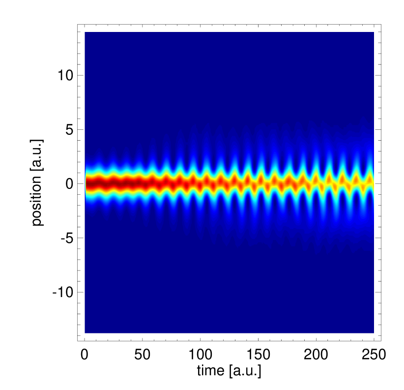
Figure 4: Time-evolution of the orbital density of the first natural orbital of Helium during the excitation from the ground state to the first excited state. The quiver motion of the electrons is nicely reflected in the density profile of the natural orbital.

We would like to thank N. Helbig, I. V. Tokatly and N. N. Lathiotakis for useful discussions. Partial financial support by the EC Nanoquanta NoE and the EXC!TING network is gratefully acknowledged.

References

- (1) Quantum Statistical Mechanics L. P. Kadanoff and G. Baym, (Benjamin, New York, 1962).
- (2) P. Danielewicz, Ann. Phys. 152, 239 (1984).
- (3) Quantum kinetic theory M. Bonitz, (Teubner, Stuttgart, 1998).
- (4) N. E. Dahlen and R. van Leeuwen, Phys. Rev. Lett. 98, 153004 (2007).
- (5) K. S. Thygesen and A. Rubio, Phys. Rev. B 77, 115333 (2008).
- (6) Time-Dependent Density Functional Theory Marques, M.A.L.; Ullrich, C.A.; Nogueira, F.; Rubio, A.; Burke, K.; Gross, E.K.U. (Eds.), (Springer-Verlag, 2006, Series: Lecture Notes in Physics, Vol. 706), 591 pages.
- (7) E. Runge and E.K.U. Gross, Phys. Rev. Lett. 52, 997 (1984).
- (8) R. van Leeuwen, Phys. Rev. Lett. 82, 3863 (1999).
- (9) D. G. Lappas and R. van Leeuwen, J. Phys. B 31, L249, (1998).
- (10) S. Goedecker and C. J. Umrigar, Phys. Rev. Lett. 81, 866 (1998).
- (11) M. A. Buijse and E. J. Baerends, Mol. Phys. 100, 401 (2002).
- (12) O. Gritsenko, K. Pernal and E. J. Baerends, J. Chem. Phys. 122, 204102 (2005).
- (13) N. Helbig, N. N. Lathiotakis, M. Albrecht, and E. K. U. Gross, Europhys. Lett. 77, 67003 (2007).
- (14) S. Sharma, J. K. Dewhurst, N. N. Lathiotakis, E. K. U. Gross, arXiv:0801.3787v2.
- (15) N. N. Bogoliubov. In G. Uhlenbeck and J. deBoer, (Ed.), Studies in Statistical Mechanics, Vol. 1, North-Holland, Amsterdam, 1961.
- (16) K. Pernal, O. Gritsenko, and E. J. Baerends, Phys. Rev. A 75, 012506 (2007).
- (17) W. Kutzelnigg and D. Mukherjee, J. Chem. Phys. 110, 2800 (1999).
- (18) M. Thiele, E.K.U. Gross and S. Kümmel, Phys. Rev. Lett. 100, 153004 (2008).
- (19) A.M.K Müller, Phys. Lett., 105A, 446 (1984).
- (20) W. Zhu, J. Botina, and H. Rabitz, J. Chem. Phys. 108, 1953 (1998); R. Kosloff, S. A. Rice, P. Gaspard, S. Tersigni and D. J. Tannor, Chem. Phys. 139, 201, (1989).
- (21) Q. Su and J. H. Eberly, Phys. Rev. A, 44, 5997 (1991).
- (22) P. Ziesche, J. Mol. Structure 527, 35 (2000).