Scaling and efficiency determine the irreversible evolution of a market

Abstract

 
Classification:
Physical Sciences/Statistics, Social Sciences/Economic Sciences

Corresponding Author:
Attilio Stella,
Dipartimento di Fisica and Sezione INFN, Università di Padova,
Via Marzolo 8, I-35131 Padova, Italy
Tel: +39 049 827 7172
Fax: +39 049 827 7102
E-mail: stella@pd.infn.it

Words and character counts:
Abstract: 130 words
Total Character Count for the manuscript: 24989

Abbreviations:
Probability density function (PDF)
Dow Jones Industrial (DJI)

Abstract:
In setting up a stochastic description of the time evolution of a financial index, the challenge consists in devising a model compatible with all stylized facts emerging from the analysis of financial time series and providing a reliable basis for simulating such series. Based on constraints imposed by market efficiency and on an inhomogeneous-time generalization of standard simple scaling, we propose an analytical model which accounts simultaneously for empirical results like the linear decorrelation of successive returns, the power law dependence on time of the volatility autocorrelation function, and the multiscaling associated to this dependence. In addition, our approach gives a justification and a quantitative assessment of the irreversible character of the index dynamics. This irreversibility enters as a key ingredient in a novel simulation strategy of index evolution which demonstrates the predictive potential of the model.

 

 

Introduction
For over a century it has been recognized bachelier_1 that the unpredictable time evolution of a financial index is inherently a stochastic process. However, in spite of many efforts mandelbrot_1 ; fama_1 ; black_1 ; engle_1 ; bollerslev_1 ; vassilicos_1 ; mandelbrot_3 ; andersen_1 ; lux_1 ; lebaron_1 , a unified framework for simultaneously understanding empirical facts mantegna_1 ; mantegna_2 ; bouchaud_2 ; cont_1 ; cont_2 ; stanley_1 ; yamasaki_1 ; lux_2 , such as the non-Gaussian form and multiscaling in time of the distribution of returns, the linear decorrelation of successive returns, and volatility clustering, has been elusive. This situation occurs in many natural phenomena, when strong correlations determine various forms of anomalous scaling kadanoff_1 ; kadanoff_2 ; sethna_1 ; bouchaud_3 ; lu_1 ; scholz_1 ; kiyono_1 ; lasinio_1 . Here, by employing novel mathematical tools at the basis of a generalization of the central limit theorem to strongly correlated variables baldovin_1 , we propose a model of index evolution and a corresponding simulation strategy which account for all robust features revealed by the empirical analysis.

Let $S(t)$ be the value of a given asset at time $t$. The logarithmic return over the interval $[t,t+T]$ is defined as $r(t,T)\equiv\ln S(t+T)-\ln S(t)$, where $t=0,1,\ldots$ and $T=1,2\ldots$, in some unit (e.g., day). From a sufficiently long historical series one can sample the empirical probability density function (PDF) of $r$ over a time $T$, $\overline{p}_{T}(r)$, and the joint PDF of two successive returns $r_{1}\equiv r(t,T)$ and $r_{2}\equiv r(t+T,T)$, denoted by $\overline{p}_{2T}^{(2)}(r_{1},r_{2})$. This joint PDF contains the information on the correlation between $r_{1}$ and $r_{2}$ in the sampling. A well established property mantegna_2 ; bouchaud_2 ; cont_1 ; cont_2 is that, if $T$ is longer than tens of minutes, the linear correlation vanishes: $\int\overline{p}_{2T}^{(2)}(r_{1},r_{2})r_{1}r_{2}dr_{1}dr_{2}\equiv\langle r_{1}r_{2}\rangle_{\overline{p}_{2T}^{(2)}}=0$. This is a consequence of the efficiency of the market fama_1 , which quickly suppresses any arbitrage opportunity. Another remarkable feature is that, within specific $T$-ranges, $\overline{p}_{T}$ approximately assumes a simple scaling form

$$\overline{p}_{T}(r)=\frac{1}{T^{\overline{D}}}\;\;\overline{g}\left(\frac{r}{T^{\overline{D}}}\right),$$ (1)

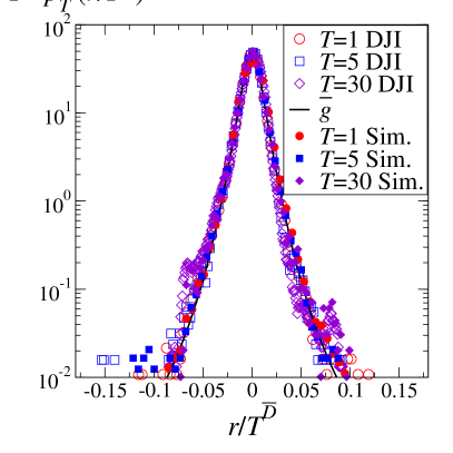
where $\overline{g}$ and $\overline{D}$ are the scaling function and exponent, respectively. Eq. (1) manifests self-similarity, a symmetry often met in natural phenomena kadanoff_1 ; kadanoff_2 ; sethna_1 ; bouchaud_3 ; lasinio_1 : plots of $T^{\overline{D}}\overline{p}_{T}$ vs $r/T^{\overline{D}}$ for different $T$’s collapse onto the same curve representing $\overline{g}$. We verify the scaling ansatz in Eq. (1) for the Dow Jones Industrial (DJI) index using a dataset of more than one century (1900-2005) of daily closures. This index is paradigmatic of market behavior and the considerable number of data reduces sampling fluctuations substantially. In Fig. 1 the collapse of the empty symbols is rather satisfactory (the explanation of the meaning of the full symbols in Fig. 1 is given below). The scaling function in Eq. (1) is non-Gaussian mandelbrot_1 ; mantegna_1 ; mantegna_2 ; bouchaud_2 ; cont_1 ; cont_2 ; stanley_1 . Although linear correlations vanish, in the $T$-range considered $\overline{g}$ is determined by the strong nonlinear correlations of the returns. Only for $T>\tau_{c}$ (with $\tau_{c}$ of the order of the year) successive index returns become independent and $\overline{p}_{T}$ turns Gaussian in force of the central limit theorem gnedenko_1 .

Results and discussion
Our first goal is to establish up to what extent the assumption of simple scaling in Eq. (1) does constrain the structure of the joint PDF $\overline{p}_{2T}^{(2)}$. One must of course have

$$\int\overline{p}_{2T}^{(2)}(r_{1},r_{2})\delta(r-r_{1}-r_{2})dr_{1}dr_{2}=\overline{p}_{2T}(r),$$

$$\int\overline{p}_{2T}^{(2)}(r_{1},r_{2})dr_{2}=\overline{p}_{T}(r_{1}),$$ (2)

$$\int\overline{p}_{2T}^{(2)}(r_{1},r_{2})dr_{1}=\overline{p}_{T}(r_{2}).$$

Indeed, the first line of Eqs. (2) follows from $r(t,2T)=r_{1}+r_{2}$. Furthermore, since the joint PDF $\overline{p}_{2T}^{(2)}$ is sampled from a sequence of time-translated intervals of duration $2T$ along the historical series, both the first and the second halves of all such intervals provide an adequate sampling basis for $\overline{p}_{T}$. This justifies the second and third lines of Eqs. (2). At this point we notice that the property $\langle r_{1}r_{2}\rangle_{\overline{p}_{2T}^{(2)}}=0$ implies that $\langle r^{2}\rangle_{\overline{p}_{2T}}=\langle(r_{1}+r_{2})^{2}\rangle_{\overline{p}_{2T}^{(2)}}=2\langle r^{2}\rangle_{\overline{p}_{T}}$. In force of Eq. (1), $\langle r^{2}\rangle_{\overline{p}_{T}}\sim T^{2\overline{D}}$. Hence, we obtain $2T^{2\overline{D}}=(2T)^{2\overline{D}}$, i.e. $\overline{D}=1/2$. Remarkably, for all developed market indices, $\langle r^{2}\rangle_{\overline{p}_{T}}$ is found to scale consistently with a $\overline{D}$ pretty close to $1/2$ di_matteo_1 .

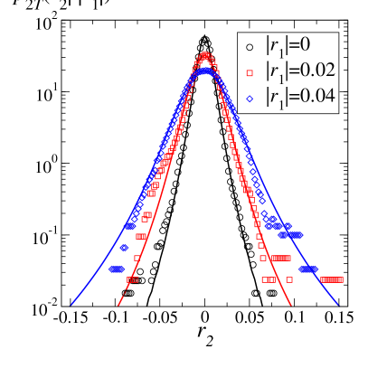
By switching to Fourier space in Eq. (2), the notion of a novel, generalized product operation allows to identify a solution for $\overline{p}_{2T}^{(2)}$ in terms of $\overline{p}_{T}$ alone. While the ordinary multiplication of characteristic functions (i.e., Fourier transforms) of Gaussian $\overline{p}_{T}$’s would yield trivially the correct $\overline{p}_{2T}^{(2)}$ in the case of independent successive returns gnedenko_1 , the generalized product is used here to take into account strong nonlinear correlations consistently with the anomalous scaling they determine (see Supporting Information) and can be seen to be at the basis of a novel central limit theorem baldovin_1 . Our solution is strongly supported by the remarkable consistency with the numerical results and by the analogy with the independent case. In Fig. 2 we compare the PDF of the return $r_{2}$ conditioned to a given absolute value of the return $r_{1}$, as obtained through our solution (continuous lines), with the empirically sampled one (symbols). The agreement does not involve fitting parameters, since $\overline{D}$ and those entering the assumed analytical form of $\overline{g}$ are already fixed in Fig. 1.

Figure 1: Data collapse for $\overline{p}_{T}(r)$ ($T$ measured in days) sampled from a record of about $2.7\times 10^{4}$ DJI daily closures (empty symbols). The average daily trend of the order of $10^{-4}$ has been subtracted. The collapse analysis furnishes the scaling function $\overline{g}$ reported as the full line and the scaling exponent $\overline{D}\simeq 1/2$ (see also Fig. 3 and Supporting Information). The full symbols report the data collapse for the results of a single simulation of the DJI history.

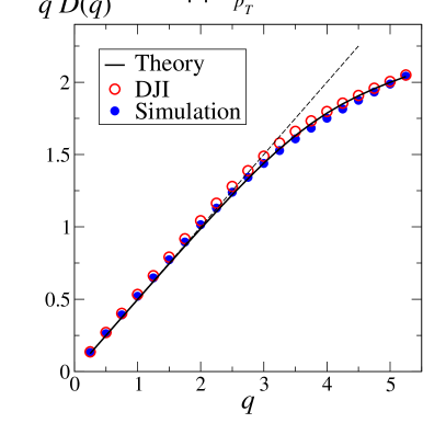
At this point we must take into account that the simple scaling ansatz in Eq. (1) is only approximately valid vassilicos_1 . Indeed, a consequence of Eq. (1) is $\langle|r|^{q}\rangle_{\overline{p}_{T}}\sim T^{q\overline{D}}$, which we exploited above for $q=2$. However, a careful analysis reveals that the $q$-th moment exponent deviates from the linear behavior $q\overline{D}\simeq q/2$ for $q\gtrsim 3$ (empty circles in Fig. 3). Like the linear behavior with slope $1/2$ observed for low-order moments, this multiscaling effect is common to most indices di_matteo_1 . To explain this feature, we have to investigate the relation between the empirical $\overline{p}_{T}$ and the stochastic process generating the time series. If PDF’s like $\overline{p}_{T}$ and $\overline{p}_{2T}^{(2)}$ were directly describing such a process, this would be with stationary increments. This assumption is legitimate only for sufficiently long times, larger than $\tau_{c}$. Below, we identify in the interplay between scaling and non-stationarity a precise mechanism accounting for the robust features of $\overline{p}_{T}$ detected for $T\ll\tau_{c}$, including its multiscaling.

Let us indicate by $p_{t,T}$ and $p_{t,2T}^{(2)}$ the ensemble PDF’s corresponding to $\overline{p}_{T}$ and $\overline{p}_{2T}^{(2)}$, respectively. The additional dependence on $t$, the initial time of the interval $[t,t+T]$, shows that we do not assume stationarity for these PDF’s. We postulate that, within specific $T$-ranges (e.g., the one in Fig. 1), $p_{0,T}$ obeys a simple scaling like that in Eq. (1), but possibly with a $D$ and a $g$ different from $\overline{D}$ and $\overline{g}$, respectively. One then realizes that this scaling and the linear decorrelation of returns impose on $p_{t,2T}^{(2)}$ constraints analogous to those for $\overline{p}_{2T}^{(2)}$ in Eq. (2), except for the third one, which now reads

$$\int p_{0,2T}^{(2)}(r_{1},r_{2})dr_{1}\equiv p_{T,T}(r_{2})=p_{0,aT}(r_{2}).$$ (3)

This last condition tells us that, as a consequence of the nonlinear correlations, the effective time span of the marginal PDF obtained by integrating $p_{0,2T}^{(2)}$ in $r_{1}$ must be renormalized by a factor $a$. This factor is determined again by consistency of the second moments scaling properties, as above. Since now $\langle|r|^{2}\rangle_{p_{0,T}}\sim T^{2D}$, one gets from Eq. (3) $a=(2^{2D}-1)^{1/2D}$. So, $D\neq 1/2$ implies $a\neq 1$ and thus non-stationarity and irreversibility of the process. Similar functional relations hold for the PDF’s of the magnetization of critical spin models upon doubling the system size and can be explained in that context by the renormalization group theory lasinio_1 . Our generalized multiplication of characteristic functions allows us to express $p_{t,2T}^{(2)}$ in terms of $p_{t,T}$ and to establish the time-inhomogeneous scaling property

$$p_{t,T}(r)=\frac{1}{\sqrt{(t+T)^{2D}-t^{2D}}}\quad g\left(\frac{r}{\sqrt{(t+T)^{2D}-t^{2D}}}\right).$$ (4)

Figure 2: Conditional probabilities of daily returns $r_{2}$ for different values of $r_{1}$. Empty symbols refer to the DJI data. The continuous curves are the predictions of our theory for $\overline{p}_{2T}^{(2)}(r_{2}||r_{1}|)\equiv[\overline{p}_{2T}^{(2)}(r_{1},r_{2})+\overline{p}_{2T}^{(2)}(-r_{1},r_{2})]/\int[\overline{p}_{2T}^{(2)}(r_{1},r_{2})+\overline{p}_{2T}^{(2)}(-r_{1},r_{2})]dr_{2}$. The absolute value of $r_{1}$ is introduced for reducing sample fluctuations.

It remains now to make explicit the link between the $p$’s and the sampled $\overline{p}$’s and to determine $D$. By construction, $\overline{p}_{T}$ is a $t$-average of $p_{t,T}$. Since the time inhomogeneity of $p_{t,T}$ must cross over into homogeneity for $t$ exceeding $\tau_{c}$, we expect the following approximation

$$\overline{p}_{T}(r)=\frac{1}{\tau_{c}}\sum_{t=0}^{\tau_{c}-1}p_{t,T}(r)$$ (5)

to hold. Indeed, the history over which $\overline{p}_{T}$ is sampled is much longer than $\tau_{c}$ and allows in principle also an indirect sampling of $p_{t,T}$ if we simply assume $p_{t+\tau_{c},T}(r)=p_{t,T}(r)$.

Figure 3: Scaling exponent of the $q$-th moment of $\overline{p}_{T}$. Empty (full) circles refer to the DJI data (simulation) of Fig. 1. The dashed line is $q/2$. Multiscaling is due to the deviation of $\overline{D}(q)$ from a constant value. The full line reports the time-averaged asymptotic ($\tau_{c}\gg 1$) theoretical prediction based on Eq. (5).

In spite of the fact that Eq. (4) implies a simple scaling exponent $D$ for $p_{0,T}$, Eq. (5) leads to the remarkable property that, independently of $D$, the low-$q$ moments of $\overline{p}_{T}$ approximately scale with exponent $q/2$ as soon as $\tau_{c}\gg 1$. Moreover, if $D<1/2$, $\overline{p}_{T}$ displays a multiscaling of the same type as that found empirically: $\overline{D}(q)<1/2$ for the high-order moments. The matching of the theoretical predictions for the multiscaling of $\overline{p}_{T}$ on the basis of Eq. (5) with the empirical results is a first way of identifying $D$. For the DJI, in Fig. 3 we show that with $D=0.24$ this matching is very satisfactory. The scaling functions of $p_{0,T}$ and $\overline{p}_{T}$ can also be shown to be simply related, once $D$ is known. We notice that the observed multiscaling features of financial indices, which inspired multiplicative cascade models mandelbrot_3 ; lux_2 in analogy with turbulence kadanoff_1 ; kadanoff_2 , are explained here in terms of an additive process possessing the time-inhomogeneous scaling (4).

Figure 4: Volatility autocorrelation at time separation $\tau$ (in days), $c(\tau)\equiv\frac{\sum_{t=0}^{t_{max}}|r(t,1)||r(t+\tau,1)|-\sum_{t=0}^{t_{max}}|r(t,1)|\sum_{t=0}^{t_{max}}|r(t+\tau,1)|/t_{max}}{\sum_{t=0}^{t_{max}}|r(t,1)|^{2}-[\sum_{t=0}^{t_{max}}|r(t,1)|]^{2}/t_{max}},$ where $t_{max}+\tau-1$ is the total length of the time series. Symbols are as in Fig. 3. The simulation here is precisely the same we refer to in Figs. 1 and 3. The full line gives the slope of the time-averaged asymptotic ($\tau_{c}\gg 1$, $\tau\lesssim\tau_{c}$) model prediction for the volatility autocorrelation, superimposed to the data (see Supporting Information).

The introduction of autoregressive schemes like ARCH engle_1 marked an advance in econometrics and financial analysis bollerslev_1 ; andersen_1 , and, more generally, in the theory of stochastic processes. In an autoregressive simulation a number of parameters weighting the influence of the past history on the PDF of the following return must be fixed through some optimization procedure. By our approach, a generalization of $p_{t,2T}^{(2)}$ to the case of $n$-consecutive intervals can be fully expressed just in terms of $p_{t,T}$ and $D$. This is obtained by taking the inverse Fourier transform of our solution for the characteristic function of the joint PDF (see Supporting Information). In this way we can precisely calculate the PDF which rules the extraction of the $i$-th return, $r_{i}$, giving as conditioning inputs the previous $m$ ones, $r_{i-m},\ldots,r_{i-1}$. Consistently with our schematization in Eq. (5), the existence of exogenous factors acting on the market can be taken into account by resetting the width of the marginal PDF’s with an (average) periodicity equal to $\tau_{c}$ (see Supporting Information). The results for a single simulation with $m=100$, $\tau_{c}=500$, and $D=0.24$ are illustrated by the full symbols in Figs. 1 and 3. The coincidence of the scaling properties observed for the DJI with those of our simulation furnish a second strong indication of the validity of our approach and of the estimation of $D$.

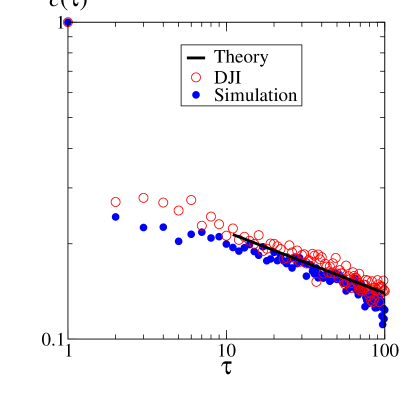
The correctness of the value of $D$ can be further checked by considering the volatility autocorrelation function at time-separation $\tau$ (Fig. 4). A well established fact mantegna_1 ; mantegna_2 ; bouchaud_2 ; cont_1 ; cont_2 ; lux_2 is its power law decay $c(\tau)\sim\tau^{-\beta}$ for $\tau<\tau_{c}$, with $\beta\simeq 0.2$ for the DJI. This behavior is not reproduced by routine simulation methods in quantitative finance like GARCH bollerslev_1 and requires the introduction of more sophisticated, fractional integration techniques andersen_1 . The full characterization of the joint PDF of $n$-consecutive returns allows us to obtain a model expression for $c(\tau)$, which again takes into account the non-stationarity of the process (see Supporting Information). Such an expression behaves asymptotically as a power of $\tau$ with an exponent depending on $D$ ($c(\tau)$ is constant for $D=1/2$ and decays for $D<1/2$). In particular, with $D=0.24$ both the model asymptotic expression and the results of our simulation procedure furnish a nice agreement with the exponent $\beta\simeq 0.2$ observed for the DJI index (Fig. 4). Thus, the algebraic volatility autocorrelation function decay is reproduced by our scheme and provides a second criterion to fix consistently the anomalous scaling exponent $D$.

Our approach is based on two postulates: inhomogeneous-time scaling and the vanishing of linear return correlations. These symmetries lead, in an unambiguous, deductive manner, to a model for the underlying stochastic process determining market evolution. Of course, the results follow only when the postulates are valid and we have shown that within specific time-ranges the consequences of these postulates are in remarkable agreement with the data. Major advances in understanding critical phenomena worked in a similar vein decades ago kadanoff_1 , when the scaling assumptions allowed to establish links between seemingly disparate phenomena and put the basis for the development of renormalization group theory lasinio_1 . So far, the coexistence of anomalous scaling with the requirement of absence of linear correlation imposed by economic principles has been regarded as an outstanding open problem in the theory of stochastic processes. We believe that our solution could be relevant for developments in this field, as well as for describing scaling behaviors of other complex systems kadanoff_1 ; kadanoff_2 ; sethna_1 ; bouchaud_3 ; lu_1 ; scholz_1 ; kiyono_1 .

Acknowledgments
We thank J.R. Banavar for useful suggestions and encouragement.

References

- (1) Bachelier, L. (1900) Ann. Sci. Ecole Norm. Sup. 17, 21-86.
- (2) Mandelbrot, B. B. (1963) J. Business 36, 394-419.
- (3) Fama, E.F. (1970) Journal of Finance 25, 383-417 .
- (4) Black F. & Scholes M. (1973) J. Polit. Econ. 81, 637-654.
- (5) Engle, R. (1983) Journal of Money, Credit and Banking 15, 286-301.
- (6) Bollerslev, T. (1986) Journal of Econometrics 31, 307-327.
- (7) Vassilicos, J. C., Demos, A. & Tata, F. (1993) in Applications of Fractals and Chaos, eds. Crilly, A. J., Earnshaw, R. A. & Jones, H. (Springer, Berlin).
- (8) Mandelbrot, B. B., Fisher, A. J. & Calvet, L. E. (1997) Cowles Foundation Discussion Paper 1164.
- (9) Andersen, T. G. & Bollerslev, T. (1997) Journal of Empirical Finance 4, 115-158.
- (10) Lux, T. & Marchesi, M. (1999) Nature 397, 498-500.
- (11) LeBaron, B. (2002) Proc. Natl. Acad. Sci. USA 99, 7201-7206.
- (12) Mantegna, R. N. & Stanley, H. E. (1995) Nature 376, 46-49.
- (13) Mantegna, R. N. & Stanley, H. E. (2000) An Introduction to Econophysics (Cambridge University Press, Cambridge, UK).
- (14) Bouchaud, J.-P. & and Potters, M., (2000) Theory of Financial Risks (Cambridge University Press, Cambridge, UK).
- (15) Cont, R. (2001) Quant. Finance 1, 223-236.
- (16) Cont, R. (2005) in Fractals in Engineering, eds. Lutton E. & Levy Véhel J. (Springer-Verlag, New York).
- (17) Stanley, H. E., Amaral, L. A. N., Buldyrev, S. V. , Gopikrishnan, P., Plerou, V., & Salinger, M. A. (2002) Proc. Natl. Acad. Sci. USA 99, 2561-2565.
- (18) Yamasaki, K., Muchnik, L., Havlin, S., Bunde, A. & Stanley H. E. (2005) Proc. Natl. Acad. Sci. USA 102, 9424-9428.
- (19) Lux, T. (in press) in Power Laws in the Social Sciences, eds. Cioffi-Revilla, C. (Cambridge University Press, Cambridge, UK).
- (20) Kadanoff, L. P. (2005) Statistical Physics, Statics, Dynamics and Renormalization, (World Scientific, Singapore).
- (21) Kadanoff, L. P. (2001) Physics Today August, 34-39.
- (22) Sethna, J. P., Dahmen, K. A. & Myers, C. R. (2001) Nature 410, 242-250.
- (23) Bouchaud, J. -P. & Georges, A. (1990) Phys. Rep. 195, 127.
- (24) Lu, E. T. , Hamilton, R. J. , McTiernan, J. M. & Bromond, K. R. (1993) Astrophys. J. 412, 841-852.
- (25) Scholz, C. H. (2002) The Mechanics of Earthquakes and Faulting (Cambridge University Press, New York).
- (26) Kiyono, K., Struzik, Z. R., Aoyagi, N., Togo, F. & Yamamoto, Y. (2005) Phys. Rev. Lett. 95, 058101.
- (27) Jona-Lasinio, G. (2001) Phys. Rep. 352, 439-458 .
- (28) Baldovin, F. & Stella, A. L. (2007) Phys. Rev. E 75, 020101(R)-1–020101(R)-4.
- (29) Gnedenko, B.V. & Kolmogorov, A.N. (1954) Limit Distributions for Sums of Independent Random Variables (Addison Wesley, Reading, MA).
- (30) Di Matteo, T, Aste, T. & Dacorogna M. M. (2005) J. Bank. & Fin. 29, 827-851.