Nonsinusoidal current-phase relation in strongly ferromagnetic and moderately disordered SFS junctions

Abstract

We study the Josephson current in a junction comprising two superconductors linked by a strong ferromagnet in presence of impurities. We focus on a regime where the electron (and hole) motion is ballistic over the exchange length and diffusive on the scale of the weak link length. The current-phase relation is obtained for both two- and three dimensional ferromagnetic weak links. In the clean limit, the possibility of temperature-induced $0$-$\pi$ transitions is demonstrated while the corresponding critical current versus temperature dependences are also studied.

I Introduction.

The Josephson effect is a striking manifestation of quantum mechanics at macroscopic scales josephson62 . When a small current $I$ is driven through a superconductor/insulator/superconductor junction, no voltage drop occurs along the junction while a finite phase difference $\chi$ appears between the two superconducting order parameters of the leads. When the applied current exceeds a maximal (critical) value $I_{c}$, a finite voltage appears across the barrier yielding a time-dependence of the phase. In many cases the stationary current phase relation (CPR) is well approximated by its first harmonic $I(\chi)=I_{1}\sin\chi$ and then the critical current is simply given by $I_{c}=I_{1}$. Nevertheless, theory gives room to higher harmonics, in particular at low temperatures. In fact, the only general requirement is that $I(\chi)$ must be a $2\pi$-periodic and odd function of the phase difference when time-reversal invariance is respected. Thus the CPR may be expressed as a Fourier sum $I(\chi)=\sum_{m}I_{m}\sin m\chi$ where the coefficients $I_{m\text{ }}$are related to processes whereby $m=1,2,..$ Cooper pairs are transferred through the weak link golubov04 .

If the junction is inserted in a superconducting loop, the supercurrent is controlled by the applied magnetic flux $\Phi$ which is directly related to the superconducting phase difference by $\chi=2\pi\Phi/\Phi_{0}$, $\Phi_{0}=h/2e$ being the superconducting flux quantum. In the absence of any bias-current or magnetic flux, the equilibrium state of a tunnel Josephson junction usually corresponds to $\chi=0$ and $I=0$. In contrast, when the tunnel barrier contains magnetic impurities, it was predicted that the phase difference may be equal to $\pi$ at equilibrium. This may enable a spontaneous persistent current to flow in a loop comprising a Josephson junction in such a $\pi$-state bulaevskii78 ; bulaevskii78ss . This $\pi$-shift is related to processes whereby electrons change their spin projection when passing through the insulating layer kulik66 ; shiba69 . Unfortunately this kind of $\pi$-state, generated by magnetic impurities in a host insulating layer, was never observed experimentally. In contrast it was further predicted buzdin82 ; buzdin82bis and observed ryazanov01 ; kontos02 that a superconductor/ferromagnetic metal/superconductor (SFS) junction also exhibits transitions between zero and $\pi$-groundstates when the exchange energy $h$ and/or the length $L$ of the ferromagnet is varied buzdin82 . The corresponding current-phase relation (CPR) $I(\chi)$ were analysed for pure buzdin82 and dirty buzdin91 ferromagnets using respectively Eilenberger and Usadel equations kopnin ; likharev79 ; buzdin05 ; lyuksyutov05 . In  both cases, the critical current of a SFS junction oscillates and decays when increasing the length or the exchange energy of the ferromagnet. The oscillations of $I_{c}(L)$ originate directly from the exchange interaction which induces a finite mismatch between the Fermi wavevectors of spin up and down electrons. Besides these oscillations, scattering by magnetic and nonmagnetic disorder strongly suppresses the critical current when $L$ is increased. In diffusive ferromagnets, this overall decay is exponential on the typical scale $\xi_{1}=\sqrt{D/h}$, $D$ being the diffusion constant. In contrast, in the pure limit, a finite Josephson current may be observed up to much larger length scales on the order of $\xi_{1}=v_{F}/T$, $v_{F\text{ }}$and $T$ being respectively the Fermi velocity in the ferromagnet and the temperature. In particular at zero temperature, the decay becomes a power law, namely $I_{c}\sim L^{-1}$ in the case of a three dimensional pure ferromagnetic weak link buzdin82 . In the absence of disorder, this critical current suppression results from the superposition of many distinct single channel CPRs associated with independent transverse channels. Accordingly this decay is expected to be less severe in low dimensional ferromagnets for it corresponds to angular averaging over quasiclassical trajectories with different angles with respect to the junction axis.

The first evidence of the $\pi$-state, in SFS junctions, came with the observation of the nonmonotonic behavior of the critical current as a function of temperature ryazanov01 and of the ferromagnet length kontos02 . The weak ferromagnetic alloys chosen for these pioneer experiments enable to observe the transitions in relatively large junctions within the ten nanometers scale. Further support was provided by magnetic diffraction patterns of DC squids comprising a SFS $\pi$-junction in one arm and a usual tunnel junction on the other arm guichard03 . Furthermore spontaneous persistent currents were reported in a loop interrupted by a $\pi$ junction bauer04 and imaged in arrays of $\pi$-Josephson junctions ryazanovNatPhys . Finally, multiple transitions between zero and $\pi$-groundstates were observed by varying the ferromagnetic layer thickness of a SFS junction oboznov06 ; robinson07 .

Experimentally obtaining the CPR is much more difficult than simply measuring the critical current. Only recently a few CPR experiments were implemented successfully in the case of SFS junctions frolov04  and SNS junctions dellarocca07 ; troeman08 ; strunk08 . In fact at sufficiently low temperature, a small second harmonic of the CPR is always present both in SNS and SFS junctions, but it is usually completely eclipsed by the large amplitude of the first harmonic. The SFS Josephson junctions are a natural playground to observe unambigously the second harmonic since the first one vanishes at the zero-$\pi$ transition. In particular, the second harmonic was detected as a tiny minimum supercurrent at the crossover between the zero and $\pi$ states, and also revealed by the related Shapiro steps sellier04 . In the highly transparent limit, the issue of the sign and magnitude of the second harmonic was adressed in presence of uniaxial buzdin05prb and isotropic houzet05 magnetic scattering in the ferromagnet. Moreover finite transparency or weak interfacial disorder may also modify the second-harmonic zareyan06 .

Zero-$\pi$ transitions were also observed in smaller junctions comprising strong ferromagnets like Fe, Co, Ni or permalloy blum02 ; robinson06 ; robinson07 . These novel experiments are performed in an interesting regime which differs both from the pure clean or dirty limits extensively studied so far. Owing to the extremelly large exchange energy, the period of the critical current oscillations $\xi_{2}=v_{F}/h$ is smaller than the mean free path $\ell=v_{F}\tau$ while the ferromagnetic bridge is still longer than the mean free path: $\xi_{2}\ll\ell\ll L$. Bergeret et al. investigated the first harmonic of the Josephson current in this particular regime $h\tau\gg 1$ bergeret01 . A theoretical analysis of this second harmonic in this particular regime is still lacking while it was already detected experimentally robinson07 .

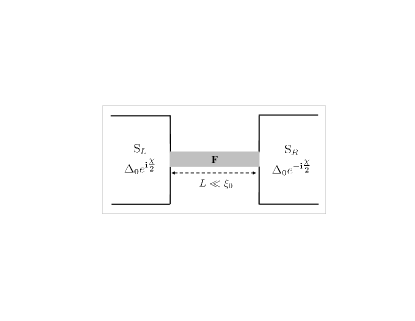
Figure 1: SFS junction. The contact area are far smaller than the typical superconducting lead ($S_{L},S_{R}$) transverse size. The metallic ferromagnet (F) in the middle part can be either two- or three- dimensional.

Up to now the physics of the $\pi$-state and second harmonic were mostly investigated in the three-dimensional case due to the lack of lower-dimensional ferromagnets. Recenlty novel systems like graphene or thin films of magnetic semiconductors became available as promising candidates for realizing two-dimensional SFS junctions. For instance coating graphene with Pd may produce itinerant magnetism uchoa08 while alcaline coating is likely to produce superconductivity uchoa07 . Hence tailoring a graphene sheet with appropriate metals on top may induce SFS heterojunctions within the carbon atoms plane. At the present time, only two experiments have been reported on SNS junctions made with graphene heersche07 ; du08 , while $0$-$\pi$ transitions were predicted in graphene based SFS junctions huertas08 . Another experiment which has triggered the interest on two-dimensional SFS junctions is the measurement of a supercurrent through a long, $L=0.3-1\mu m$, half-metallic ferromagnet chromium oxide (CrO${}_{2\text{ }}$) film keiser06 wherein singlet superconductivity should be destroyed on a much smaller length scale. The spin singlet to triplet conversion (at the interfaces) was proposed to explain the finite Josephson current. It was shown that triplet correlations penetrate a ferromagnet on much longer distances bergeret05 . Another possibility is that the surface of the film is less spin-polarized than the bulk or even antiferromagnetically ordered. In this latter scenario, a singlet supercurrent may bypass the half-metallic ferromagnet by flowing within a two-dimensional SFS surface junction.

In this paper, we study both two- and three-dimensional SFS junctions with strong exchange field and moderate disorder, namely in the limit $h\tau\gg 1$. Using Eilenberger equations and perturbative expansion in $1/h\tau$, we obtain the current phase relation and in particular its second-harmonic at the $0$-$\pi$ transition which was recently observed in the three-dimensional case robinson07 . In the pure limit, we show that the two-dimensional critical current is suppressed as $L^{-1/2}$ instead of $L^{-1}$ in the three-dimensional case. Accordingly we suggest the possibility to observe enhanced critical current in planar SFS junctions made of magnetic semiconductors or graphene with an induced ferromagnetic order.

After introducing the formalism in Sec. II, we investigate the pure limit in Sec. III with special emphasis on the two-dimensional case and on temperature-induced $0$-$\pi$ transitions. In Sec IV, the CPR of two- and three-dimensional SFS junctions are obtained in the limit $h\tau\gg 1$ in relation with experiments robinson07 .

II SFS model and formalism.

We study a superconductor-ferromagnetic-superconductor (SFS) Josephson junction in the geometry represented in Fig.1. The ferromagnet consists in a single ferromagnetic domain characterized by its exchange energy $h$, length $L=L_{x}$ and transverse dimension(s) $L_{y}$ (and $L_{z}$). We assume that the superconducting order parameter is $\Delta_{0}e^{i\chi/2}$ (resp. $\Delta_{0}e^{-i\chi/2}$) in the left (right) superconducting lead while the Fermi velocity $v_{F}$ is the same everywhere. The contacts between superconductors and the ferromagnet are completely transparent and spin inactive. Besides the geometrical parameters of the junction, three typical lengths are of primary importance for the Josephson effect. On the one hand the superconducting coherence length $\xi_{0}=v_{F}/\pi\Delta_{0}$ and the ferromagnetic exchange length $\xi_{F}=v_{F}/h$ are related to the strengh of the superconducting and ferromagnetic order parameters respectively. On the other hand disorder is characterized by the elastic mean free path $\ell=v_{F}\tau$ where $\tau$ is the average time between impurity scattering events. Henceforth, we adopt units with $\hbar=k_{B}=1$.

Previous theoretical studies were mostly performed in the diffusive limit $\ell\ll\xi_{F},L$ or in the pure limit $\ell\gg\xi_{F},L$ using respectively the Usadel and the Eilenberger equations (without self-energy terms due to disorder) kopnin . Recent experiments have opened to possibility to investigate the regime $\xi_{F}\ll\ell\ll L$ blum02 ; robinson06 ; robinson07 . This later regime cannot be described by the Usadel equation since the disorder induced self-energy is no longer the dominant energy. It is thus necessary to use the Eilenberger formalism bergeret01  and the exchange energy as the large parameter which enable perturbative expansions.

In our simple model, the quasi-classical Eilenberger Green functions $g=g_{\omega}\left(x,v_{x}\right)$, $f=f_{\omega}\left(x,v_{x}\right)$ and $f^{+}=f_{\omega}^{+}\left(x,v_{x}\right)$ depend only on the center-of-mass coordinate $x$ along the junction axis $Ox,$ and on the angle $\theta$ of the quasiclassical trajectories with respect to $Ox$.

In the ferromagnetic weak link, $\left|x\right|<L/2$, the Eilenberger equations read

$$\left\{\begin{array}[c]{l}v_{x}\partial_{x}g=\left(2\tau\right)^{-1}\left(f\left\langle f^{+}\right\rangle-f^{+}\left\langle f\right\rangle\right),\\ v_{x}\partial_{x}f=-2\left(\omega+ih\right)+\dfrac{1}{\tau}\left(g\left\langle f\right\rangle-f\left\langle g\right\rangle\right),\\ -v_{x}\partial_{x}f^{+}=-2\left(\omega+ih\right)f^{+}+\dfrac{1}{\tau}\left(g\left\langle f^{+}\right\rangle-f^{+}\left\langle g\right\rangle\right).\end{array}\right.$$ (1)

Here $\omega=\pi T\left(2n+1\right)$ are the Matsubara frequencies and $v_{x}=v_{F}\cos\theta$ is the Fermi velocity vector kopnin . The brackets denote averaging over the Fermi surface.

In the superconducting leads, which are assumed to be clean, the Eilenberger equations read :

$$\left\{\begin{array}[c]{l}v_{x}\partial_{x}g=\Delta^{\ast}f-\Delta f^{+}\\ v_{x}\partial_{x}f=-2\omega f+2\Delta g\\ v_{x}\partial_{x}f^{+}=2\omega f^{+}-2\Delta^{\ast}g\end{array}\right.$$ (2)

with $\Delta=\Delta_{0}e^{i\chi/2}$ (resp. $\Delta_{0}e^{-i\chi/2}$) for the left (resp. right) electrode respectively. In the whole paper, $\Delta_{0}=1,764T_{c}\tanh\left(1,74\sqrt{T/T_{c}-1}\right)$ is the temperature dependent superconducting gap.

In the limit $h\tau\gg 1$ studied thorough this paper, one may assumes as a starting approximation that $\left\langle f\right\rangle=\left\langle f^{+}\right\rangle=0$. Then demanding the continuity of the general solutions of Eqs. ($\ref{EQ_eilenberger_ferro},\ref{EQ_eilenberger_supra})$ at the interfaces $x=\pm L/2$ yields the quasiclassical Green functions over the whole junction. In particular, in the ferromagnet, $\left|x\right|<L/2$, one finds that the normal Green function

$$g\left(x,v_{x}\right)=\frac{\omega}{\Omega}+\frac{\Delta_{0}^{2}}{\Omega}\frac{\sinh\Phi}{\omega\sinh\Phi\pm\Omega\cosh\Phi}$$ (3)

is independent of the position $x$. The upper (lower) sign of the denominator corresponds to the positive (negative) sign in the velocity projection. We have defined $\Omega^{2}=\omega^{2}+\Delta_{0}^{2}$ and the effective phase

$$\Phi=\dfrac{\omega L}{v_{x}}+\frac{\left\langle g\right\rangle L}{2v_{x}\tau}+i\left(\dfrac{hL}{v_{x}}+\dfrac{\chi}{2}\right)$$ (4)

which contains all the relevant parameters of the junction. In experiments, the exchange field $h$ is always larger than the temperature, and thus the contribution $\omega L/v_{x}$ may be safely neglected in the above expression for $\Phi$.

The supercurrent density is given by the following quasiclassical expression kopnin

$$j\left(\chi\right)=2\pi e\nu_{0}^{\left(d\right)}T\sum_{\omega}\left\langle v_{x}\operatorname{Im}g_{\omega}\left(v_{x}\right)\right\rangle$$ (5)

where the temperature $T$ is expressed in energy units and $\nu_{0}^{\left(d\right)}$ is the density of state at the Fermi level per spin and per unit volume (resp. surface) for $d=3$ (resp. $d=2$). The corresponding current $\ I\left(\chi\right)$ is obtained as the flux of $j\left(\chi\right)$ through a section of the weak link.

Finally the groundstate energy $E_{\chi}$ of the junction can be deduced by integrating the CPR according to the general formula

$$I\left(\chi\right)=\frac{2\pi}{\Phi_{0}}\frac{\partial E_{\chi}}{\partial\chi},$$ (6)

where $\Phi_{0}=h/2e$ is the superconducting flux quantum. The $0-\pi$ phase transition occurs when the $\chi=0$ and $\chi=\pi$ groundstates are degenerate, namely when $E_{0}=E_{\pi}$.

III SFS junction in the pure limit.

In this section, we consider the pure limit $L\ll\ell$ with special emphasis on the two-dimensional case. Indeed, the three-dimensional and the one-dimensional cases are well known for both small buzdin82 and large cayssol04 ; cayssol05 exchange energies. After briefly recalling the single channel results, we obtain that the low temperature critical current of a two-dimensional Josephson junction decays as $L^{-1/2}$, namely more slowly than the $L^{-1}$ dependence characterizing three-dimensional ballistic weak links. We obtain the CPR and study the second harmonic at the $0$-$\pi$ transition, where the first harmonic cancels. We also study the possibility of $\ 0$-$\pi$ transitions induced by varying the temperature at a given length. Finally, the $I_{c}(T)$ curves are obtained and compared to recent experiments oboznov06 ; robinson07 .

III.1 Single channel case.

State of the art ferromagnetic wires typically still contain a large number of transverse channels. Nevertheless, the analysis of the single channel case is both necessary and instructive since, in the ballistic limit, it is the building block for evaluating the multichannel supercurrent in higher dimensions. When considering a single transverse channel, the angular averaging $\left\langle..\right\rangle$ in Eq.$\left(\ref{EQ_current_definition}\right)$ reduces to a discrete sum over $\theta=0$ and $\theta=\pi$ which yields the following current-phase relation:

$$I\left(\chi\right)=I_{0}^{\left(1\right)}\sum_{\sigma=\pm 1}\tanh\left(\dfrac{\Delta_{0}}{2T}\cos\dfrac{\chi+\sigma\alpha}{2}\right)\sin\dfrac{\chi+\sigma\alpha}{2},$$ (7)

where $\alpha=2hL/v_{F}$ and $I_{0}^{\left(1\right)}=e\nu_{0}^{\left(1\right)}\pi v_{F}\Delta_{0}$. Using Eq.$\left(\ref{EQ_def_energy}\right)$, one obtains the energy of the junction

$$\frac{E_{\chi}\left(\alpha,T\right)}{E_{0}^{\left(1\right)}}=-\sum_{\sigma=\pm 1}\ln\left[\cosh\left(\dfrac{\Delta_{0}}{2T}\cos\dfrac{\chi+\sigma\alpha}{2}\right)\right]$$ (8)

as a function of the phase difference $\chi$. The typical energy scale is given by $E_{0}^{\left(1\right)}=2T\pi\nu_{0}^{\left(1\right)}\hslash v_{F}$. The $\chi=0$ and $\pi$ groundstates are degenerate for regularly spaced values of the accumulated phase $\alpha$, namely at $\alpha_{n}=\pi/2+n\pi$. These critical values of the parameter $\alpha$ can be reached by varying either the length $L$ or the exchange energy $h,$ whereas they are insensitive to temperature variation. Hence in an hypothetical single channel SFS junction, it would be impossible to drive the $0$-$\pi$ transition by varying the temperature only.

Close to the critical temperature, $T\approx T_{c}$, the linearization of Eq.$\left(\ref{EQ_monocanal_current}\right)$ yields a nearly sinusoidal current-phase relation $I\left(\chi\right)=I_{c}(\alpha)\sin\chi$ whose critical current, $I_{c}(\alpha)=I_{0}^{\left(1\right)}(\Delta_{0}/2T_{c})\cos\alpha$, cancels for $\alpha=\pi/2+n\pi$, namely at the $0$-$\pi$ transitions. Moreover the oscillatory behavior of $I_{c}(\alpha)$ is not damped when $\alpha,$ or equivalently $L$ and/or $h$, are increased. This behaviour is due to the absence of angular averaging in the single channel situation.

At lower temperatures, $T\ll T_{c}$, the CPR becomes nonsinusoidal. The corresponding critical current $I_{c}\left(\alpha\right)$ is obtained numerically by maximazing the current density $I\left(\chi\right)$ given by Eq.$\left(\ref{EQ_monocanal_current}\right)$. This critical current $I_{c}(\alpha)$ also exhibits periodic oscillations as a function of $\alpha=2hL/v_{F}$. In contrast to the situation for $T\approx T_{c}$, the current $I_{c}\left(\alpha\right)$ is finite at the cusps owing to the presence of a sizeable second harmonic. Finally, it is very instructive to check the sign of this second harmonic $I_{2}(\alpha_{n})$ at the zero-$\pi$ transitions where first harmonic cancels $I_{1}(\alpha_{n})=0,$ since this sign is related to the order of the transition. It turns out that $I_{2}(\alpha_{n})>0$ which yields a discontinuous (first-order) phase transition between the $0$ to the $\pi$ phases. Otherwise, namely for $I_{2}(\alpha_{n})<0$, the transition would have been continuous (second-order) with a groundstate corresponding to an arbitrary value of the phase difference, distinct from $0$ or $\pi$ buzdin05 .

III.2 Two-dimensional case.

In a two-dimensional SFS junction, the supercurrent is the sum of the currents carried by independent transverse modes. Using the angular averaging $\left\langle..\right\rangle=\int d\theta/2\pi(..)$ appropriate for planar junctions, one obtains the following CPR:

$$I\left(\chi\right)=I_{0}^{\left(2\right)}\sum_{\sigma=\pm 1}\int_{\alpha}^{\infty}\frac{\alpha^{2}dy}{y^{2}\sqrt{y^{2}-\alpha^{2}}}\times\\ \times\tanh\left(\frac{\Delta_{0}}{2T}\cos\frac{\chi+\sigma y}{2}\right)\sin\frac{\chi+\sigma y}{2}$$ (9)

where $\alpha=2hL/v_{F}$ and $I_{0}^{\left(2\right)}=e\nu_{0}^{\left(2\right)}\pi v_{F}\Delta_{0}$. The corresponding critical current $I_{c}\left(\alpha\right)$ is shown in Fig.2 for several temperatures. In contrast to the single channel case, the oscillations of $I_{c}(\alpha)$ are damped due to the angular averaging over many transverse channels having each a distinct CPR. For $T<T_{c}$, the curves $I_{c}(\alpha)$ exhibit cusps where the critical current remains finite instead of the cancellations observed for $T\approx T_{c}$.

The zero- and $\pi$-groundstate energies $E_{0}(\alpha)$ and $E_{\pi}(\alpha)$ depend both of $\alpha$ and temperature according to:

$$\frac{E_{0}\left(\alpha\right)}{E_{0}^{\left(3\right)}} =-2\int_{\alpha}^{\infty}\ln\left[\cosh\left(\frac{\Delta_{0}}{2T}\cos\frac{y}{2}\right)\right]\frac{\alpha^{2}dy}{y^{2}\sqrt{y^{2}-\alpha^{2}}},$$ (10)

$$\frac{E_{\pi}\left(\alpha\right)}{E_{0}^{\left(3\right)}} =-2\int_{\alpha}^{\infty}\ln\left[\cosh\left(\frac{\Delta_{0}}{2T}\sin\frac{y}{2}\right)\right]\frac{\alpha^{2}dy}{y^{2}\sqrt{y^{2}-\alpha^{2}}}.$$ (11)

The values of the parameter $\alpha=2hL/v_{F}$ where the $\left(0\text{-}\pi\right)$ transitions occur are obtained by solving $E_{0}(\alpha)=E_{\pi}(\alpha)$ which may be rewritten as

$$\int_{\alpha_{c}}^{\infty}\ln\frac{\cosh\left(\dfrac{\Delta_{0}}{2T}\cos\dfrac{y}{2}\right)}{\cosh\left(\dfrac{\Delta_{0}}{2T}\sin\dfrac{y}{2}\right)}\frac{dy}{y^{2}\sqrt{y^{2}-\alpha_{c}^{2}}}=0.$$ (12)

At low temperature $T<T_{c},$ we have checked that the solutions $\alpha_{c}(T)$ for Eq.(12) coincide with the location of the cusps in the $I_{c}\left(\alpha\right)$ curves. Moreover, $\alpha_{c}(T)$ decreases when the temperature is lowered, see Fig. 2. The phase diagram in the $\alpha$-$T$ plane is similar than the three dimensional phase diagram shown in Fig.4. It should be also emphasized that this transition is not accompanied by a non-monotonic behavior of the $I_{c}\left(T\right)$ curves in contrast to the dirty case oboznov06 .

Figure 2: Critical current as a function of $\alpha=2hL/v_{F}$ in a two-dimensional SFS junction. The temperature is increased from the upper curve ($T\approx 0$) to the lower one ($T\approx T_{c}$).  The $0-\pi$ phase transitions occur at the kinks of the $I_{c}(\alpha)$ curve. For a given $0-\pi$ transition, the positions of $\alpha_{n}(T)$ of these kinks exhibit weak temperature dependence.

Near the critical temperature $T_{c},$ the current-phase relation is nearly sinusoidal with a first harmonic given by

$$I_{1}(\alpha)=I_{0}^{\left(2\right)}\dfrac{\Delta_{0}}{2T_{c}}\int_{\alpha}^{\infty}dy\frac{\alpha^{2}\cos y}{y^{2}\sqrt{y^{2}-\alpha^{2}}},$$ (13)

and a second harmonic given by:

$$I_{2}(\alpha)\approx-\frac{I_{0}^{\left(2\right)}}{12}\left(\dfrac{\Delta_{0}}{2T}\right)^{3}\int_{\alpha}^{\infty}dy\frac{\alpha^{2}\cos 2y}{y^{2}\sqrt{y^{2}-\alpha^{2}}}.$$ (14)

Both $I_{1}(\alpha)$ and $I_{1}(\alpha)$ exhibit an oscillatory dependence on $\alpha$, see Fig.3. In the limit $\alpha\gg 1$, the asympotic behaviors are given respectively by

$$\frac{I_{1}(\alpha,T\rightarrow T_{c})}{I_{0}^{\left(2\right)}}\approx\dfrac{\Delta_{0}}{2T_{c}}\frac{\sqrt{\pi}}{2}\frac{\cos\alpha-\sin\alpha}{\sqrt{\alpha}}$$ (15)

and by:

$$\frac{I_{2}(\alpha,T\rightarrow T_{c})}{I_{0}^{\left(2\right)}}\approx-\left(\dfrac{\Delta_{0}}{2T_{c}}\right)^{3}\frac{\sqrt{\pi}}{24}\frac{\cos 2\alpha-\sin 2\alpha}{\sqrt{2\alpha}}$$ (16)

Thus in the regime $\alpha\gg 1$, the $0$-$\pi$ transitions occur for the values $\alpha=\pi/4+n\pi$ where the first harmonic of the CPR cancels. Moreover the second harmonic is positive at these transitions.

Figure 3: Critical current $I_{c}\left(\alpha\right)$ versus $\alpha=2hL/v_{F}$ for $T\approx T_{c}$ , from Eq.$\left(\ref{EQ_critical_current_near_Tc_2D}\right)$ in the two-dimensional case (solid curve) and from Eq.$\left(\ref{EQ_critical_current_near_Tc_3D}\right)$ in the three-dimensional case (dashed curve). In the two-dimensional case, the period of $I_{c}$ is larger than in the three-dimensional case. The overall decay of $I_{c}$ is also much slower in the two dimensional case.

III.3 Three-dimensional case.

Finally we consider the well-known CPR for three-dimensional SFS junctions buzdin82 :

$$I\left(\chi\right)=I_{0}^{\left(3\right)}\sum_{\sigma=\pm 1}\int_{\alpha}^{\infty}\frac{\alpha^{2}dy}{y^{3}}\times\\ \times\tanh\left(\frac{\Delta_{0}}{2T}\cos\frac{\chi+\sigma y}{2}\right)\sin\frac{\chi+\sigma y}{2}$$ (17)

in order to compare with the two-dimensional results described in the previous paragraph. Here $I_{0}^{\left(3\right)}=e\nu_{0}^{\left(3\right)}L_{y}L_{z}\pi v_{F}\Delta_{0}$ and $E_{0}^{\left(3\right)}=2T\pi\nu_{0}^{\left(3\right)}\hslash v_{F}$. The zero- and $\pi-$groundstate energies $E_{0}(\alpha)$ and $E_{\pi}(\alpha)$ depend both of $\alpha$ and temperature according to:

$$\frac{E_{0}\left(\alpha\right)}{E_{0}^{\left(3\right)}} =-2\int_{\alpha}^{\infty}\ln\left[\cosh\left(\frac{\Delta_{0}}{2T}\cos\frac{y}{2}\right)\right]\frac{\alpha^{2}dy}{y^{3}},$$ (18)

$$\frac{E_{\pi}\left(\alpha\right)}{E_{0}^{\left(3\right)}} =-2\int_{\alpha}^{\infty}\ln\left[\cosh\left(\frac{\Delta_{0}}{2T}\sin\frac{y}{2}\right)\right]\frac{\alpha^{2}dy}{y^{3}}.$$ (19)

By solving numerically $E_{0}\left(\alpha\right)=E_{0}\left(\alpha\right)$ at arbitrary temperature, we obtain the curves $\alpha_{c}(T)$ shown in Fig.4. In principle, the system can experience $0-\pi$ phase transition by lowering the temperature at some given $\alpha$, provided this value of $\alpha$ is close to a critical value. It is important to note that the range wherein the $\left(0-\pi\right)$ phase transition can take place by tuning the temperature is smaller for the three-dimensional case than in the two-dimensional one.

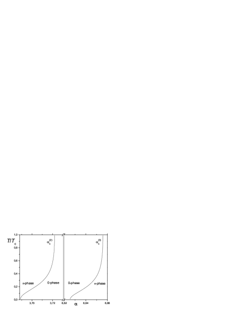
Figure 4: Phase diagram in the $\alpha$-$T$ plane showing the transition lines between the $0$ and the $\pi$ phases for a three dimensional SFS junction. We have used $\Delta_{0}\left(T\right)=1,764T_{c}\tanh\left(1,74\sqrt{T/T_{c}-1}\right)$.

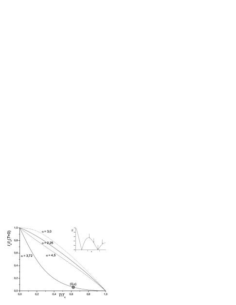
Figure 5: Critical current $I_{c}\left(T\right)$ versus temperature for a three-dimensional junction. Four different values of $\alpha=2hL/v_{F}$ are shown: $\alpha=2.25$ (solid line), $\alpha=3.0$ (dotted line), $\alpha=3.72$ (solid line) and $\alpha=4,5$ (dashed line). The critical current decreases monotonically when the temperature is increased. The dot on the $\alpha=3.72$ curve indicates the $\left(0\text{-}\pi\right)$ transition, which is not associated with any singular behavior in the $I_{c}\left(T\right)$ curve. In the inset, the above values of $\alpha$ are indicated on the $I_{c}\left(\alpha,T\rightarrow T_{c}\right)$ curve.

Near the critical temperature $T_{c},$ the first harmonic is given by

$$I_{c}(\alpha)=I_{0}^{\left(3\right)}\dfrac{\Delta_{0}}{2T_{c}}\int_{\alpha}^{\infty}\cos y\frac{\alpha^{2}dy}{y^{3}}$$ (20)

which is plotted on Fig.3. The asympotic behaviors are given by

$$I_{1}(\alpha,T\rightarrow T_{c})\approx-I_{0}^{\left(3\right)}\dfrac{\Delta_{0}}{2T_{c}}\frac{\sin\alpha}{\alpha}$$ (21)

in the limit $\alpha\gg 1$.The second harmonic

$$I_{2}(\alpha,T\rightarrow T_{c})\approx\frac{I_{0}^{\left(3\right)}}{12}\left(\dfrac{\Delta_{0}}{2T_{c}}\right)^{3}\frac{\sin 2\alpha}{2\alpha}\text{ \ \ }$$ (22)

also exhibits an oscillatory dependence with respect to $\alpha$. Thus in the regime $\alpha\gg 1$ and close to $T_{c}$, the $0$-$\pi$ transitions occur for the values $\alpha_{n}=n\pi$ where the first harmonic of the CPR cancels. The second harmonic is positive at those points, $I_{2}(n\pi)>0$, indicating first order transitions.

III.4 Temperature dependence $I_{c}(T)$

For appropriate values of the ferromagnetic layer length and exchange energy (corresponding to $\alpha=\alpha_{n}$), it is possible to pass through the $0-\pi$  transition point by changing the temperature, as shown in Figs.4 and 5 for $\alpha=3.72.$ This kind of temperature induced $0-\pi$ transition was actually achieved in experiments using dirty weakly ferromagnetic alloys oboznov06 . It was observed that the critical current exhibits a nonmonotonic $T$-dependence with a cancellation at the $0-\pi$ transition. Moreover the $\pi$ state can be either the low (e.g. at the first node) or the high temperature phase (at second node) oboznov06 . In contrast, only monotonic variations of $I_{c}(T)$ were reported in experiments with strong ferromagnets in the clean (or moderately dirty) limit robinson07 ; blum02 .

Here we have obtained that, in the pure limit, the critical current does decrease monotonously when the temperature is increased, as shown in Fig.5. Nevertheless the temperature dependence of the critical current $I_{c}(T)$ exhibits very distinct shapes (e.g. in Fig.5 for $\alpha=3$ and $\alpha=3.72$) being either convexe, concave or almost linear depending on the value of $\alpha=2Lh/v_{F}$. Although we have shown extreme cases (in Fig.5 for $\alpha=3$ and $\alpha=3.72$), most of our $I_{c}(T)$ curves are almost linear in agreement with the experimental curves reported in robinson07 ; blum02 . For future experiments, we suggest the observation of the concave curves (e.g. $\alpha=3.72$ in Fig.5) as a signature of the $0$-$\pi$ transition. The corresponding measure is quite challenging since it corresponds to the temperature dependence of a minimum of the critical current which is given only by the contributions of higher harmonics ($m\geqslant 2$). Similar features were predicted in the limit of large exchange fields using Bogoliubov-de Gennes formalism cayssol05 . Here we confirm that this change in the concavity of the $I_{c}(T)$ curve near a $0$-$\pi$ transition is still predicted in the limit of moderate exchange fields in comparison to the Fermi energy. In contrast, the $I_{c}(T)$ curves are non monotonic in the dirty limit when the junction passes the $0$-$\pi$ transition. We explain this discrepancy by the fact that the critical current at the $0$-$\pi$ transition vanishes in the dirty limit whereas it is still finite in the pure limit (due to the important contribution of high harmonics).

IV SFS junction with impurities.

Experiments on SFS junctions comprising dilute magnetic alloys are correctly described within the Usadel equation framework oboznov06 ; buzdin05prb ; houzet05 ; zareyan06 ; cottet05 , because the exchange energy is smaller than the disorder level broadening, namely $\tau h\ll 1$, and far smaller than the Fermi energy. In this regime the electron (and hole) motion is diffusive with a mean free path smaller than both $\xi_{F}$ and $L$. Recently experiments were performed in the opposite regime, $\tau h\gtrsim 1$, using strong ferromagnets, like Fe, Co, Ni or Permalloy. Then the electron (and hole) motion is ballistic over the ferromagnetic length scale $\xi_{F}$, while being still diffusive on the scale of the weak link length $L$. In particular this situation implies that the parameter $\alpha=2L/\xi_{F}$ is very large. The first harmonic of the CPR for three dimensional weak links has been already found buzdin82bis ; bergeret01 by solving the Eilenberger equations for large $\tau h$. In this section, we calculate the amplitudes of the first and second harmonic both in two- and three- dimensional SFS junctions. The analytical expressions obtained here can be used as a starting point to interpret the three-dimensional experiments by Robinson et al. robinson07 and future investigations on graphene-based SFS junctions huertas08 .

IV.1 Three dimensional case.

Here we investigate the CPR $\ I(\chi)=I_{1}\sin\chi+I_{2}\sin 2\chi+...$ of a three dimensional junction. We have obtained the first harmonic

$$I_{1}=8\text{ }I_{0}^{\left(3\right)}T\sum_{\omega>0}\frac{\Delta_{0}}{(\omega+\Omega)^{2}}\operatorname{Re}E_{3}(z),$$ (23)

and the second harmonic

$$I_{2}=8I_{0}^{\left(3\right)}T\sum_{\omega>0}\frac{\Delta_{0}^{3}}{(\omega+\Omega)^{4}}\operatorname{Re}\left(\frac{L}{l}E_{2}^{2}(z)-E_{3}(2z)\right),$$ (24)

where $I_{0}^{\left(3\right)}=e\nu_{0}^{\left(3\right)}L_{y}L_{z}\pi v_{F}\Delta_{0}$, $L_{y}L_{z}$ being the junction area, and $z=L/l+i\alpha=L/l+2iL/\xi_{F}$. The functions $E_{i}(z)$ are defined in the appendix. The first harmonic corresponds to the result previously obtained in buzdin82bis ; bergeret01 . The second harmonic is usually smaller than the first one, except when $I_{1}$ cancels. Then we obtain that the magnitude of $I_{2}$ is perfectly measurable though small. Moreover, the sign of $I_{2}$ when $I_{1}=0$ is very instructive since it determines the order of the transition. When the first harmonic cancels, the second harmonic is finite and positive. This is the usual case where one observes a discontinuous jump of the junction between the zero and $\pi$ states. For negative $I_{2}$ when $I_{1}=0$, one would expect a continuous transition and the realisation of a $\varphi$ junction buzdin05 . For the experimentally relevant regime of moderate $L/l$, we always obtain that the second harmonic is positive at the transition (see Fig. 6). For larger values of $L/l$, we have also observed negative $I_{2}$ although numerical artefact cannot be excluded.

We now study how the supercurrent is suppressed when the weak link length or the exchange field is increased. The asymptotic behaviors of the harmonics at $\alpha\gg 1$ are given by

$$\frac{I_{1}}{I_{0}^{\left(3\right)}}=\text{ }T\sum_{\omega>0}\frac{8\Delta_{0}e^{-L/l}}{(\omega+\Omega)^{2}}\operatorname{Re}\left(\frac{e^{-2iL/\xi_{F}}}{L/l+2iL/\xi_{F}}\right),$$ (25)

and

$$\frac{I_{2}}{I_{0}^{\left(3\right)}}=T\sum_{\omega>0}\frac{8\Delta_{0}^{3}e^{-2L/l}}{(\omega+\Omega)^{4}}\operatorname{Re}\left(\frac{(L/l-2iL/\xi_{F})e^{-4iL/\xi_{F}}}{(L/l+2iL/\xi_{F})^{2}}\right),$$ (26)

Besides the exponential suppression $I_{1}\sim e^{-L/l}$ (and $e^{-2L/l}$ for $I_{2}$), the real parts in Eq.(25,26) provide damped oscillations as a function of $\alpha$, as shown in Fig. 7.

The sum over Matsubara frequencies yields the temperature dependence of the harmonics. At low temperature $T\rightarrow 0$, the sum over Matsubara frequencies becomes an integral that can be done analytically yielding:

$$\frac{I_{1}}{I_{0}^{\left(3\right)}}=\frac{8}{3}\operatorname{Re}\left(\frac{e^{-2iL/\xi_{F}}}{L/l+2iL/\xi_{F}}\right)e^{-L/l},$$ (27)

and

$$\frac{I_{2}}{I_{0}^{\left(3\right)}}=\frac{8}{15}\operatorname{Re}\left(\frac{(L/l-2iL/\xi_{F})e^{-4iL/\xi_{F}}}{(L/l+2iL/\xi_{F})^{2}}\right)e^{-2L/l},$$ (28)

at large $\alpha$.

IV.2
Two dimensional case.

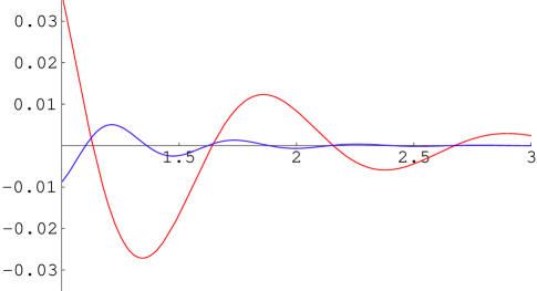
Figure 6: First (red curve) and second (blue curve) harmonic as functions of $L/l$ for a three-dimensional junction. We have chosen $l/\xi_{F}=5$. The corresponding analytical expressions Eqs.(23,24) are derived in the regime $\xi_{F}\lesssim l\lesssim L$. Hence the lower limit for $L/l$ is one.

For planar junctions, both the first and second harmonics were unknown in the strong ferromagnet regime $\xi_{F}\ll l\ll L$. Using the procedure described in appendix, we have evaluted these harmonics as

$$I_{1}=16\text{ }I_{0}^{\left(2\right)}T\sum_{\omega>0}\frac{\Delta_{0}}{(\omega+\Omega)^{2}}\operatorname{Re}F_{2}(z),$$ (29)

and

$$I_{2}=16\text{ }I_{0}^{\left(2\right)}T\sum_{\omega>0}\frac{\Delta_{0}^{3}}{(\omega+\Omega)^{4}}\operatorname{Re}\left(\frac{L}{l}F_{1}^{2}(z)-F_{2}\left(2z\right)\right).$$ (30)

Here $I_{0}^{\left(2\right)}=e\nu_{0}^{\left(2\right)}\pi v_{F}\Delta_{0}L_{y}$, $L_{y}$ being the width of the planar weak link, and $z=L/l+2iL/\xi_{F}$. The functions $F_{i}(z)$ are defined in the appendix. From Fig.7, one obseves that the second harmonic is finite and positive when the first harmonic cancels.

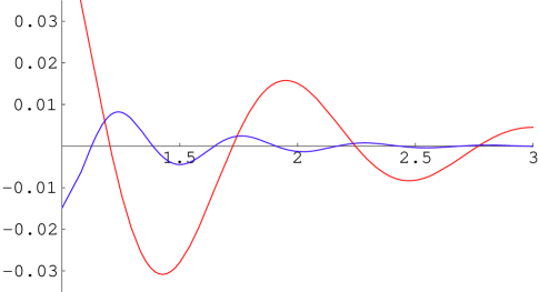
Figure 7: First (red curve) and second (blue curve) harmonic as functions of $L/l$ for a two-dimensional junction. We have chosen $l/\xi_{F}=5$. The corresponding analytical expressions Eqs.(29,30) are derived in the regime $\xi_{F}\lesssim l\lesssim L$. Hence the lower limit for $L/l$ is one.

IV.3 Comparison with experiments

In the experiments robinson07 , the values of the parameter $h\tau$ are respectively $h\tau=3$ for Ni₈₀Fe₂₀, $2.8$ for Co, $1.62$ for Fe and $0.5$ for Ni, using the parameters ($h,v_{F},l$) provided in robinson07 . The experiments blum02 performed on Nb-Ni-Nb junctions correspond to $h\tau\simeq 1$. Hence these experiments cover the onset of the regime $h\tau\geq 1$, or equivalently $\xi_{F}\lesssim l$. The oscillations of the critical current are reported for weak link lengths $L$ not exceeding few mean free paths $l$, othewise the signal would be too small (due to the exponential suppression by the factor $e^{-L/l}$). The period of the oscillations is approximatively $0.5$ in units of $L/l$ in agreement with our results for $h\tau=3$, see Fig. 7. Quantitative comparison between our theory and these experiments are hindered by the fact that band structure effects and interface quality may strongly influence the magnitude of the Josephson current.

V Conclusion.

In the absence of impurities, we have demonstated that temperature-induced $0$-$\pi$ transitions are possible both in two and three dimensional SFS junctions though it requires weak exchange fields in practice. The overall decay or damping of the critical current as a function of the length/exchange field of the ferromagnet is much slower ($L^{-1/2}$) in the two-dimensional case than in the three dimensional case ($L^{-1}$). Moreover, the shape of the critical current versus temperature curves changes when one closely approaches a $0$-$\pi$ transition. Hence for future experiments, we suggest the challenging measure of the temperature dependence of a minimum of the critical current, which is essentially given by the contributions of higher harmonics ($m\geqslant 2$). The corresponding $I_{c}(T)$ should differ markedly form the usual almost linear curves obtained so far away from those minima robinson07 ; blum02 .

We have obtained the current phase relation for SFS junctions comprising strong ferromagnets in the presence of moderate disorder, namely in the limit $\tau h\gtrsim 1$. We have calculated the second harmonic, in particular at the $0$-$\pi$ transition, for both two- and three- dimensional SFS junctions. In the three dimensional case, we have compared our result with recent experiments performed in the regime $\tau h\gtrsim 1$ robinson07 .

VI Appendix.

In this appendix, we derive the current-phase relation in the regime $L\gg\ell\gg\xi_{F},$ or equivalently $\alpha\gg\tau h\gg 1$. We start with the normal quasiclassical Green function which is uniform in the ferromagnet:

$$g_{\omega}\left(\theta\right)=\frac{\omega}{\Omega}+\frac{\Delta_{0}^{2}}{\Omega}\frac{\sinh\Phi(\theta)}{\omega\sinh\Phi(\theta)\pm\Omega\cosh\Phi(\theta)},$$ (31)

where $+/-$ corresponds to the sign of $\cos\theta$ and

$$2\Phi(\theta)=i\chi+\frac{\left\langle g\right\rangle L/l+i\alpha}{\cos\theta}$$ (32)

with $\alpha=2hL/v_{F}$. We first consider the case of positive Matsubara frequency $\omega>0$. Then, one expands $g_{\omega}\left(\theta\right)$ in powers of $X_{\lambda}=\exp\left[-2\lambda\Phi(\theta)\right]$ as

$$g_{\omega}\left(\theta\right)=1-\frac{2\Delta_{0}^{2}}{(\omega+\Omega)^{2}}X_{\lambda}+\frac{2\Delta_{0}^{4}}{(\omega+\Omega)^{4}}X_{\lambda}^{2}+...$$ (33)

where $\lambda$ is the sign of $\cos\theta$. The modulus of $X_{\lambda}$ is a small parameter because $\left|X_{\lambda}\right|=\exp(-2\lambda\left\langle g\right\rangle L/(l\cos\theta))$ with $\left\langle g\right\rangle>0$ (In first approximation $\left\langle g\right\rangle=sgn(\omega)$) and $L\gg l$. This expansion defines a self-consistent problem since $X_{\lambda}$ contains $\left\langle g\right\rangle$ which in turn is evaluated using $X_{\lambda}$. As a first iteration, we evaluate $g_{\omega}\left(\theta\right)$ using $\left\langle g\right\rangle=1$ in the expression of $X_{\lambda}$. Then we perform the angular averaging to obtain the first order correction to $\left\langle g\right\rangle$. Denoting $\left\langle g\right\rangle=1+g_{1}$ ( $\left|g_{1}\right|\ll 1$) one obtains, in the three dimensional case:

$$g_{1} =-\frac{2\Delta_{0}^{2}\cos\chi}{(\omega+\Omega)^{2}}{\displaystyle\int\limits_{0}^{\pi/2}}d\theta\sin\theta\exp\left(-\frac{z}{\cos\theta}\right)$$ (34)

$$=-\frac{2\Delta_{0}^{2}\cos\chi}{(\omega+\Omega)^{2}}E_{2}(z)$$ (35)

with $z=L/l+i\alpha$ and $E_{n}(z)={\displaystyle\int\limits_{1}^{\infty}}dy$ $y^{-n}e^{-zy}$.

The current is related to the quantity:

$$\left\langle v_{x}g_{\omega}\left(\theta\right)\right\rangle =-\frac{v_{F}\Delta_{0}^{2}}{(\omega+\Omega)^{2}}{\displaystyle\int\limits_{0}^{\pi/2}}d\theta\sin\theta\cos\theta(X_{\oplus}-X_{\ominus})$$ (36)

$$+\frac{v_{F}\Delta_{0}^{4}}{(\omega+\Omega)^{4}}{\displaystyle\int\limits_{0}^{\pi/2}}d\theta\sin\theta\cos\theta(X_{\oplus}^{2}-X_{\ominus}^{2})$$

In this expression, the first integral (proportional to $\Delta_{0}^{2}$) must be evaluated within the approximation:

$$X_{\oplus}-X_{\ominus}=-2i\sin\chi\exp\left(-\frac{z}{\cos\theta}\right)\left(1-g_{1}\frac{L/l}{\cos\theta}\right),$$ (37)

whereas the zero-order approximation $\left\langle g\right\rangle=1:$

$$X_{\oplus}^{2}-X_{\ominus}^{2}=-2i\sin 2\chi\exp\left(-\frac{2z}{\cos\theta}\right)$$ (38)

is sufficient for the second integral (proportional to $\Delta_{0}^{4}$). Substituing Eq.(37,38) in Eq.(36) yields:

$$\left\langle v_{x}g_{\omega}\left(\theta\right)\right\rangle =\frac{2iv_{F}\Delta_{0}^{2}}{(\omega+\Omega)^{2}}E_{3}(z)\sin\chi$$

$$+\frac{2iv_{F}\Delta_{0}^{4}}{(\omega+\Omega)^{4}}\left(\frac{L}{l}E_{2}^{2}(z)-E_{3}(2z)\right)\sin 2\chi\text{ }$$

and finally Eq.(23,24).

In the two dimensional case, the first order correction to $\left\langle g\right\rangle$ reads:

$$g_{1} =-\frac{2\Delta_{0}^{2}\cos\chi}{\pi(\omega+\Omega)^{2}}{\displaystyle\int\limits_{0}^{\pi/2}}d\theta\exp\left(-\frac{L/l+i\alpha}{\cos\theta}\right)$$ (39)

$$=-\frac{2\Delta_{0}^{2}\cos\chi}{(\omega+\Omega)^{2}}F_{1}(z)\text{,}$$ (40)

where:

$$F_{n}(z)={\displaystyle\int\limits_{1}^{\infty}}\frac{dye^{-zy}}{\pi y^{n}\sqrt{y^{2}-1}}.$$ (41)

The current is related to the average:

$$\left\langle v_{x}g_{\omega}\left(\theta\right)\right\rangle =v_{F}{\displaystyle\int\limits_{0}^{\pi/2}}\frac{d\theta}{\pi}\cos\theta\left[g(\theta)-g(\pi-\theta)\right]$$

$$=-\frac{2v_{F}\Delta_{0}^{2}}{(\omega+\Omega)^{2}}{\displaystyle\int\limits_{0}^{\pi/2}}\frac{d\theta}{\pi}\cos\theta(X_{\oplus}-X_{\ominus})$$

$$+\frac{2v_{F}\Delta_{0}^{4}}{(\omega+\Omega)^{4}}{\displaystyle\int\limits_{0}^{\pi/2}}\frac{d\theta}{\pi}\cos\theta(X_{\oplus}^{2}-X_{\ominus}^{2}).$$

Proceeding to the same approximations as for the three-dimensional case, one obtains:

$$\left\langle v_{x}g_{\omega}\left(\theta\right)\right\rangle =\frac{4i\sin\chi v_{F}\Delta_{0}^{2}}{(\omega+\Omega)^{2}}F_{2}(z)\mathbf{+}$$

$$+\frac{4i\sin 2\chi v_{F}\Delta_{0}^{4}}{(\omega+\Omega)^{4}}\left(\frac{L}{l}F_{1}^{2}(z)-F_{2}\left(2z\right)\right)\text{ }$$

and finally Eqs.(29,30).

- (1) B. Josephson, Phys. Lett. 1, 251 253 ( 1962).
- (2) A. Golubov, M. Kupriyanov, and E. Il’ichev, Rev. Mod. Phys. 76, 411 (2004).
- (3) L. N. Bulaevskii, V. V. Kuzii, and A. A. Sobyanin, Pis’ma Zh. ksp. Teor. Fiz. 25, 314 (1977) [JETP Lett. 25, 290 (1977)].
- (4) L.N. Bulaevskii, V.V. Kuzii, and A.A. Sobyanin, Solid State Commun. 25, 1053 (1978).
- (5) I.O. Kulik, JETP 22, 841 (1966).
- (6) H. Shiba and T. Soda, Prog. Theor. Phys., 41, 25, (1969).
- (7) A.I. Buzdin, L.N. Bulaevskii, and S.V. Panyukov, JETP Lett. 35, 178 (1982).
- (8) A.I. Buzdin, L.N. Bulaevskii, and S.V. Panyukov, Solid State Commun. 44, 539 (1982).
- (9) V. V. Ryazanov, V. A. Oboznov, A. Yu. Rusanov, A. V. Veretennikov, A. A. Golubov, and J. Aarts, Phys. Rev. Lett. 86, 2427 (2001).
- (10) T. Kontos, M. Aprili, J. Lesueur, F. Genet, B. Stephanidis, and R. Boursier, Phys. Rev. Lett. 89, 137007 (2002).
- (11) A.I. Buzdin and M.Y. Kuprianov, JETP Lett. 53, 308 (1991).
- (12) N.B. Kopnin, in Theory of Nonequilibrium Superconductivity. The International Series of Monographs on Physics, Vol. 110 (Clarendon Oxford, 2001).
- (13) K.K. Likharev, Rev. Mod. Phys. 51, 101 (1979).
- (14) A. I. Buzdin, Rev. Mod. Phys. 77, 935 (2005).
- (15) I. F. Lyuksyutov and V. L. Pokrovsky, Adv. Phys. 54, 67 (2005).
- (16) W. Guichard, M. Aprili, O. Bourgeois, T. Kontos, J. Lesueur, and P. Gandit, Phys. Rev. Lett. 90, 167001 (2003).
- (17) A. Bauer, J. Bentner, M. Aprili, M.L. Della Rocca, M. Reinwald, W. Wegscheider, and C. Strunk, Phys. Rev. Lett. 92, 217001 (2004).
- (18) S.M. Frolov, M.J.A. Stoutimore, T.A. Crane, D.J. Van Harlingen, V.A. Oboznov, V.V. Ryazanov, A. Ruosi, C. Granata, and M. Russo, Nature Physics 4, 32 (2008).
- (19) V. A. Oboznov, V. V. Bolginov, A. K. Feofanov, V. V. Ryazanov, and A. I. Buzdin, Phys. Rev. Lett 96, 197003 (2006).
- (20) J. W.A. Robinson, S. Piano, G. Burnell, C. Bell, and M. G. Blamire, Phys. Rev. B 76, 094522 (2007).
- (21) S.M. Frolov, D.J. Van Harlingen, V.A. Oboznov, V.V. Bolginov, and V.V. Ryazanov, Phys. Rev. B 70, 144505 (2004).
- (22) M.L. Della-Rocca, M. Chauvin, B. Huard, H. Pothier, D. Esteve and C. Urbina, Phys. Rev. Lett. 99, 127005 (2007).
- (23) A. G.P. Troeman, S. H. van der Ploeg, E. Il Ichev, H.-G. Meyer, A. A. Golubov, M. Yu. Kupriyanov, and H. Hilgenkamp, Phys. Rev. B 77, 024509 (2008).
- (24) M. Fuechsle, J. Bentner, D.A. Ryndyk, M. Reinwald, W. Wegscheider, and C. Strunk, arXiv0707.4512
- (25) Hermann Sellier, Claire Baraduc, Fran ois Lefloch, and Roberto Calemczuk , Phys. Rev. Lett. 92, 257005 (2004).
- (26) A. Buzdin, Phys. Rev. B 72, 100501(R) (2005).
- (27) M. Houzet, V. Vinokur, and F. Pistolesi, Phys. Rev. B 72, 220506(R) (2005).
- (28) G. Mohammadkhani and M. Zareyan, Phys. Rev. B 73, 134503 (2006).
- (29) Y. Blum, A. Tsukernik, M. Karpovski, and A. Palevski, Phys. Rev. Lett. 89, 187004 (2002).
- (30) J. W.A. Robinson, S. Piano, G. Burnell, C. Bell, and M. G. Blamire, Phys. Rev. Lett. 97, 177003 (2006).
- (31) F. S. Bergeret, A. F. Volkov, and K. B. Efetov, Phys. Rev. B 64, 134506 (2001).
- (32) B. Uchoa, C-Y. Lin, and A.H. Castro Neto, Phys. Rev. B 77, 035420 (2008).
- (33) B. Uchoa and A.H. Castro Neto, Phys. Rev. Lett. 98, 146801 (2007).
- (34) H.B. Heersche, P. Jarillo-Herrero, J.B. Oostinga, L.M.K. Vandersypen and A.F. Morpurgo, Nature 446 , 56 (2007).
- (35) Xu Du, Ivan Skachko, and Eva Y. Andrei , Phys. Rev. B 77, 184507 (2008).
- (36) J. Linder, T. Yokoyama, D. Huertas-Hernando, and A. Sudbo, Phys. Rev. Lett. 100, 187004 (2008).
- (37) R.S. Keiser, S.T.B Goennenwein, T.M. Klapwijk, G. Miao, G. Xiao, and A. Gupta, Nature 439, 825 (2006).
- (38) F. S. Bergeret, A. F. Volkov, and K. B. Efetov, Rev. Mod. Phys. 77, 1321 (2005).
- (39) J. Cayssol and G. Montambaux, Phys. Rev. B 70, 224520 (2004).
- (40) J. Cayssol and G. Montambaux, Phys. Rev. B 71, 012507 (2005).
- (41) A. Cottet and W. Belzig, Phys. Rev. B 72, 180503(R) (2005).