An ESPRIT-based Approach for Initial Ranging in OFDMA Systems

Abstract

This work presents a novel Initial Ranging scheme for orthogonal frequency-division multiple-access networks. Users that intend to establish a communication link with the base station (BS) are normally misaligned both in time and frequency and the goal is to jointly estimate their timing errors and carrier frequency offsets with respect to the BS local references. This is accomplished with affordable complexity by resorting to the ESPRIT algorithm. Computer simulations are used to assess the effectiveness of the proposed solution and to make comparisons with existing alternatives.

1 Introduction

A major impairment in orthogonal frequency-division multiple-access (OFDMA) networks is the remarkable sensitivity to timing errors and carrier frequency offsets (CFOs) between the uplink signals and the base station (BS) local references. For this reason, the IEEE 802.16e-2005 standard for OFDMA-based wireless metropolitan area networks (WMANs) specifies a synchronization procedure called Initial Ranging (IR) in which subscriber stations that intend to establish a link with the BS transmit pilot symbols on dedicated subcarriers using specific ranging codes. Once the BS has detected the presence of these pilots, it has to estimate some fundamental parameters of ranging subscriber stations (RSSs) such as timing errors, CFOs and power levels.

Initial synchronization and power control in OFDMA was originally discussed in [1] and [2] while similar solutions can be found in [3]-[4]. A different IR approach has recently been proposed in [5]. Here, each RSS transmits pilot streams over adjacent OFDMA blocks using orthogonal spreading codes. As long as channel variations are negligible over the ranging period, signals of different RSSs can be easily separated at the BS as they remain orthogonal after propagating through the channel. Timing information is eventually acquired in an iterative fashion by exploiting the autocorrelation properties of the received samples induced by the use of the cyclic prefix (CP).

All the aforementioned schemes are derived under the assumption of perfect frequency alignment between the received signals and the BS local reference. However, the occurrence of residual CFOs results into a loss of orthogonality among ranging codes and may compromise the estimation accuracy and detection capability of the IR process. Motivated by the above problem, in the present work we propose a novel ranging scheme for OFDMA networks with increased robustness against frequency errors and lower computational complexity than the method in [5]. To cope with the large number of parameters to be recovered, we adopt a three-step procedure. In the first step the number of active codes is estimated by resorting to the minimum description length (MDL) principle [6]. Then, the ESPRIT (Estimation of Signal Parameters by Rotational Invariance Techniques) [7] algorithm is employed in the second and third steps to detect which codes are actually active and determine their corresponding timing errors and CFOs.

2 System description and signal model

2.1 System description

We consider an OFDMA system employing $N$ subcarriers with index set $\{0,1,\ldots,N-1\}$. As in [5], we assume that a ranging time-slot is composed by $M$ consecutive OFDMA blocks where the $N$ available subcarriers are grouped into ranging subchannels and data subchannels. The former are used by the active RSSs to complete their ranging processes, while the latter are assigned to data subscriber stations (DSSs) for data transmission. We denote by $R$ the number of ranging subchannels and assume that each of them is divided into $Q$ subbands. A given subband is composed of a set of $V$ adjacent subcarriers which is called a tile. The subcarrier indices of the $q$th tile $(q=0,1,\ldots,Q-1)$ in the $r$th subchannel $(r=0,1,\ldots,R-1)$ are collected into a set $\mathcal{J}_{q}^{(r)}=\{i_{q}^{(r)}+v\}_{v=0}^{V-1}$, where the tile index $i_{q}^{(r)}$ can be chosen adaptively according to the actual channel conditions. The only constraint in the selection of $i_{q}^{(r)}$ is that different tiles must be disjoint, i.e., $\mathcal{J}_{q_{1}}^{(r_{1})}\cap\mathcal{J}_{q_{2}}^{(r_{2})}=\varnothing$ for $q_{1}\neq q_{2}$ or $r_{1}\neq r_{2}$. The $r$th ranging subchannel is thus composed of $QV$ subcarriers with indices in the set $\mathcal{J}^{(r)}=\cup_{q=0}^{Q-1}{\mathcal{J}_{q}^{(r)}}$, while a total of $N_{R}=QVR$ ranging subcarriers is available in each OFDMA block.

We assume that each subchannel can be accessed by a maximum number of $K_{\max}=\min\{V,M\}-1$ RSSs, which are separated by means of orthogonal codes in both the time and frequency domains. The codes are selected in a pseudo-random fashion from a predefined set $\{\mathbf{C}_{0},\mathbf{C}_{1},\ldots,\mathbf{C}_{K_{\max}-1}\}$ with

$$\mathbf{[C}_{k}\mathbf{]}_{v,m}=e^{j2\pi k(\frac{v}{V-1}+\frac{m}{M-1})}$$ (1)

where $v=0,1,\ldots,V-1$ counts the subcarriers within a tile and is used to perform spreading in the frequency domain, while $m=0,1,\ldots,M-1$ is the block index by which spreading is done in the time domain across the ranging time-slot. As in [5], we assume that different RSSs select different codes. Also, we assume that a selected code is employed by the corresponding RSS over all tiles in the considered subchannel. Without loss of generality, we concentrate on the $r$th subchannel and denote by $K\leq K_{\max}$ the number of simultaneously active RSSs. To simplify the notation, the subchannel index ^(r) is dropped henceforth.

The signal transmitted by the $k$th RSS propagates through a multipath channel characterized by a channel impulse response (CIR) $\mathbf{h}^{\prime}_{k}=[h^{\prime}_{k}(0),h^{\prime}_{k}(1),\ldots,h^{\prime}_{k}(L-1)]^{T}$ of length $L$ (in sampling periods). We denote by $\theta_{k}$ the timing error of the kth RSS expressed in sampling intervals $T_{s}$, while $\varepsilon_{k}$ is the frequency offset normalized to the subcarrier spacing. As discussed in [8], during IR the CFOs are only due to Doppler shifts and/or to estimation errors and, in consequence, they are assumed to lie within a small fraction of the subcarrier spacing. Timing offsets depend on the distance of the RSSs from the BS and their maximum value is thus limited to the round trip delay from the cell boundary. In order to eliminate interblock interference (IBI), we assume that during the ranging process the CP length comprises $N_{G}\geq\theta_{\max}+L$ sampling periods, where $\theta_{\max}$ is the maximum expected timing error. This assumption is not restrictive as initialization blocks are usually preceded by long CPs in many standardized OFDMA systems.

2.2 System model

We denote by $\mathbf{X}_{m}(q)=[X_{m}(i_{q}),X_{m}(i_{q}+1),\ldots,X_{m}(i_{q}+V-1)]^{T}$ the discrete Fourier transform (DFT) outputs corresponding to the $q$th tile in the $m$th OFDMA block. Since DSSs have successfully completed their IR processes, they are perfectly aligned to the BS references and their signals do not contribute to $\mathbf{X}_{m}(q)$. In contrast, the presence of uncompensated CFOs destroys orthogonality among ranging signals and gives rise to interchannel interference (ICI). The latter results in a disturbance term plus an attenuation of the useful signal component. To simplify the analysis, in the ensuing discussion the disturbance term is treated as a zero-mean Gaussian random variable while the signal attenuation is considered as part of the channel impulse response. Under the above assumptions, we may write

$$X_{m}(i_{q}+v)=\sum\limits_{k=1}^{K}\mathbf{[C}_{\ell_{k}}\mathbf{]}_{v,m}{e^{j{m\omega_{k}N_{T}}}}H_{k}(\theta_{k},{\varepsilon_{k},}i_{q}+v)+w_{m}(i_{q}+v)$$ (2)

where $\omega_{k}=2\pi\varepsilon_{k}/N$, $N_{T}=N+N_{G}$ denotes the duration of the cyclically extended block and $\mathbf{C}_{\ell_{k}}$ is the code matrix selected by the kth RSS. The quantity $H_{k}(\theta_{k},{\varepsilon_{k},}n)$ is the $k$th equivalent channel frequency response over the $n$th subcarrier and is given by

$$H_{k}(\theta_{k},{\varepsilon_{k},}n)=\gamma_{N}({\varepsilon_{k})}H_{k}^{\prime}(n)e^{-j{2\pi n\theta_{k}}/N}$$ (3)

where $H_{k}^{\prime}(n)=\sum_{\ell=0}^{L-1}h_{k}^{\prime}(\ell)e^{-j{2\pi n\ell}/N}$ is the true channel frequency response, while

$$\gamma_{N}({\varepsilon})=\frac{\sin(\pi{\varepsilon})}{N\sin(\pi{\varepsilon}/N)}e^{j\pi{\varepsilon}(N-1)/N}$$ (4)

is the attenuation factor induced by the CFO. The last term in (2) accounts for background noise plus interference and is modeled as a circularly symmetric complex Gaussian random variable with zero-mean and variance $\sigma_{w}^{2}=\sigma_{n}^{2}+\sigma_{ICI}^{2}$, where $\sigma_{n}^{2}$ and $\sigma_{ICI}^{2}$ are the average noise and ICI powers, respectively. From (3) we see that $\theta_{k}$ appears only as a phase shift across the DFT outputs. The reason is that the CP duration is longer than the maximum expected propagation delay.

To proceed further, we assume that the tile width is much smaller than the channel coherence bandwidth. In this case, the channel response is nearly flat over each tile and we may reasonably replace the quantities $\{H_{k}^{\prime}(i_{q}+v)\}_{v=0}^{V-1}$ with an average frequency response

$$\overline{H}_{k}^{\prime}(q)=\frac{1}{V}\sum_{v=0}^{V-1}H_{k}^{\prime}(i_{q}+v).$$ (5)

Substituting (1) and (3) into (2) and bearing in mind (5), yields

$$X_{m}(i_{q}+v)=\sum\limits_{k=1}^{K}{e^{j2\pi({m\xi_{k}+v\eta}_{k}{)}}}S_{k}(q)+w_{m}(i_{q}+v)$$ (6)

where $S_{k}(q)=\gamma_{N}({\varepsilon_{k})}\overline{H}_{k}^{\prime}(q)e^{-j{2\pi i}_{q}{\theta_{k}}/N}$ and we have defined the quantities

$$\xi_{k}=\frac{\ell_{k}}{M-1}+\frac{\varepsilon_{k}N_{T}}{N}$$ (7)

and

$$\eta_{k}=\frac{\ell_{k}}{V-1}-\frac{\theta_{k}}{N}$$ (8)

which are referred to as the effective CFOs and timing errors, respectively.

In the following sections we show how the DFT outputs $\{X_{m}(i_{q}+v)\}$ can be exploited to identify the active codes and to estimate the corresponding timing errors and CFOs.

3 ESPRIT-based estimation

3.1 Determination of the number of active codes

The first problem to solve is to determine the number $K$ of active codes over the considered ranging subchannel. For this purpose, we collect the $(i_{q}+v)$th DFT outputs across all ranging blocks into an M-dimensional vector $\mathbf{Y}(i_{q,v})=[X_{0}(i_{q}+v),X_{1}(i_{q}+v),\ldots,X_{M-1}(i_{q}+v)]^{T}$ given by

$$\mathbf{Y}(i_{q,v})=\sum_{k=1}^{K}e^{j2\pi v\eta_{k}}S_{k}(q)\mathbf{e}_{M}(\xi_{k})+\mathbf{w}(i_{q,v})$$ (9)

where $\mathbf{w}(i_{q,v})=[w_{0}(i_{q}+v),w_{1}(i_{q}+v),\ldots,w_{M-1}(i_{q}+v)]^{T}$ is Gaussian distributed with zero mean and covariance matrix $\sigma_{w}^{2}\mathbf{I}_{M}$ while $\mathbf{e}_{M}(\xi)=[1,e^{j2\pi\xi},e^{j4\pi\xi},\ldots,e^{j2\pi(M-1)\xi}]^{T}$.

From the above equation, we observe that $\mathbf{Y}(i_{q,v})$ has the same structure as measurements of multiple uncorrelated sources from an array of sensors. Hence, an estimate of $K$ can be obtained by performing an eigendecomposition (EVD) of the correlation matrix $\mathbf{R}_{Y}=\mathrm{E}\{\mathbf{Y}(i_{q,v})\mathbf{Y}^{H}(i_{q,v})\}$. In practice, however, $\mathbf{R}_{Y}$ is not available at the receiver and must be replaced by some suitable estimate. One popular strategy to get an estimate of $\mathbf{R}_{Y}$ is based on the forward-backward (FB) principle. Following this approach, $\mathbf{R}_{Y}$ is replaced by $\hat{\mathbf{R}}_{Y}=\frac{1}{2}(\tilde{\mathbf{R}}_{Y}+\mathbf{J}\tilde{\mathbf{R}}_{Y}^{T}\mathbf{J})$, where $\tilde{\mathbf{R}}_{Y}$ is the sample correlation matrix

$$\tilde{\mathbf{R}}_{Y}=\frac{1}{QV}\sum_{v=0}^{V-1}\sum_{q=0}^{Q-1}\mathbf{Y}(i_{q,v})\mathbf{Y}^{H}(i_{q,v})$$ (10)

while $\mathbf{J}$ is the exchange matrix with 1’s on the anti-diagonal and 0’s elsewhere. Arranging the eigenvalues $\hat{\lambda}_{1}\geq\hat{\lambda}_{2}\geq\cdots\geq\hat{\lambda}_{M}$ of $\hat{\mathbf{R}}_{Y}$ in non-increasing order, we can find an estimate $\hat{K}$ of the number of active codes by applying the MDL information-theoretic criterion. This amounts to looking for the minimum of the following objective function [6]

$$\mathcal{F(}\tilde{K})=\frac{1}{2}\tilde{K}(2V-\tilde{K})\ln(MQ)-MQ(V-\tilde{K})\ln\rho(\tilde{K})$$ (11)

where $\rho(\tilde{K})$ is the ratio between the geometric and arithmetic means of $\{\hat{\lambda}_{\tilde{K}+1},\hat{\lambda}_{\tilde{K}+2},\ldots,\hat{\lambda}_{M}\}$.

3.2 Frequency estimation

For simplicity, we assume that the number of active codes has been perfectly estimated. An estimate of ${\boldsymbol{\xi}}{=[}\xi_{1},\xi_{2},\ldots,\xi_{K}\mathbf{]}^{T}$ can be found by applying the ESPRIT algorithm to the model (9). To elaborate on this, we arrange the eigenvectors of $\hat{\mathbf{R}}_{Y}$ associated to the $K$ largest eigenvalues $\hat{\lambda}_{1}\geq\hat{\lambda}_{2}\geq\cdots\geq\hat{\lambda}_{K}$ into an $M\times K$ matrix $\mathbf{Z}=[\mathbf{z}_{1}~{}\mathbf{z}_{2}~{}\cdots\mathbf{z}_{K}]$. Next, we consider the matrices $\mathbf{Z}_{1}$ and $\mathbf{Z}_{2}$ that are obtained by collecting the first $M-1$ rows and the last $M-1$ rows of $\mathbf{Z}$, respectively. The entries of ${\boldsymbol{\xi}}$ are finally estimated in a decoupled fashion as

$$\hat{\xi}_{k}=\frac{1}{2\pi}\arg\{\rho_{y}(k)\}\text{ \ \ \ \ }k=1,2,\ldots,K$$ (12)

where $\{\rho_{y}(1),\rho_{y}(2),\ldots,\rho_{y}(K)\}$ are the eigenvalues of

$$\mathbf{Z}_{Y}=(\mathbf{Z}_{1}^{H}\mathbf{Z}_{1})^{-1}\mathbf{Z}_{1}^{H}\mathbf{Z}_{2}$$ (13)

and $\arg\{\rho_{y}(k)\}$ denotes the phase angle of $\rho_{y}(k)$ taking values in the interval $[-\pi,\pi)$.

After computing estimates of the effective CFOs through (12), the problem arises of matching each $\hat{\xi}_{k}$ to the corresponding code $\mathbf{C}_{\ell_{k}}$. This amounts to finding an estimate of $\ell_{k}$ starting from $\hat{\xi}_{k}$. For this purpose, we denote by $\left|\varepsilon_{\max}\right|$ the magnitude of the maximum expected CFO and observe from (7) that $(M-1)\xi_{k}$ belongs to the interval $I_{\ell_{k}}=[\ell_{k}-\beta;\ell_{k}+\beta]$, with $\beta=\left|\varepsilon_{\max}\right|N_{T}(M-1)/N$. It follows that the effective CFOs can be univocally mapped to their corresponding codes as long as $\beta<1/2$ since only in that case intervals $\{I_{\ell_{k}}\}_{k=1}^{K}$ are disjoint. The acquisition range of the frequency estimator is thus limited to $\left|\varepsilon_{\max}\right|<N/(2N_{T}(M-1))$ and an estimate of the pair $(\ell_{k},\varepsilon_{k})$ is computed as

$$\hat{\ell}_{k}=\text{round}\left((M-1)\hat{\xi}_{k}\right)$$ (14)

and

$$\hat{\varepsilon}_{k}=\frac{N}{N_{T}}\left(\hat{\xi}_{k}-\frac{\hat{\ell}_{k}}{M-1}\right).$$ (15)

It is worth noting that the $\arg\{\cdot\}$ function in (12) has an inherent ambiguity of multiples of $2\pi$, which translates into a corresponding ambiguity of the quantity $\hat{\ell}_{k}$ by multiples of $M-1$. Hence, recalling that $\ell_{k}\in\{0,1,\ldots,K_{\max}-1\}$ with $K_{\max}<M$, a refined estimate of $\ell_{k}$ can be found as

$$\hat{\ell}_{k}^{(F)}=[\hat{\ell}_{k}]_{M-1}$$ (16)

where $[x]_{M-1}$ is the value of $x$ reduced to the interval $[0,M-2]$. In the sequel, we refer to (15) as the ESPRIT-based frequency estimator (EFE).

3.3 Timing estimation

We call $\mathbf{X}_{m}(q)=[X_{m}(i_{q}),X_{m}(i_{q}+1),\ldots,X_{m}(i_{q}+V-1)]^{T}$ the $V$-dimensional vector of the DFT outputs corresponding to the qth tile in the mth OFDMA block. Then, from (6) we have

$$\mathbf{X}_{m}(q)=\sum\limits_{k=1}^{K}{e^{j2\pi{m\xi_{k}}}}S_{k}(q)\mathbf{e}_{V}(\eta_{k})+\mathbf{w}_{m}(q)$$ (17)

where $\mathbf{w}_{m}(q)=[w_{m}(i_{q}),w_{m}(i_{q}+1),\ldots,w_{m}(i_{q}+V-1)]^{T}$ is Gaussian distributed with zero mean and covariance matrix $\sigma_{w}^{2}\mathbf{I}_{V}$ while $\mathbf{e}_{V}(\eta)=[1,e^{j2\pi\eta},e^{j4\pi\eta},\ldots,e^{j2\pi(V-1)\eta}]^{T}$. Since $\mathbf{X}_{m}(q)$ is a superposition of complex sinusoidal signals with random amplitudes embedded in white Gaussian noise, an estimate of ${\boldsymbol{\eta}}{=[}\eta_{1},\eta_{2},\ldots,\eta_{K}\mathbf{]}^{T}$ can still be obtained by resorting to the ESPRIT algorithm. Following the previous steps, we first compute $\hat{\mathbf{R}}_{X}=\frac{1}{2}(\tilde{\mathbf{R}}_{X}+\mathbf{J}\tilde{\mathbf{R}}_{X}^{T}\mathbf{J})$ with

$$\tilde{\mathbf{R}}_{X}=\frac{1}{MQ}\sum_{m=0}^{M-1}\sum_{q=0}^{Q-1}\mathbf{X}_{m}(q)\mathbf{X}_{m}^{H}(q).$$ (18)

Then, we define a $V\times K$ matrix $\mathbf{U}=[\mathbf{u}_{1}~{}\mathbf{u}_{2}~{}\cdots\mathbf{u}_{K}]$ whose columns are the eigenvectors of $\hat{\mathbf{R}}_{X}$ associated to the $K$ largest eigenvalues. The effective timing errors are eventually estimated as

$$\hat{\eta}_{k}=\frac{1}{2\pi}\arg\{\rho_{x}(k)\},\text{ \ \ \ \ }k=1,2,\ldots,K$$ (19)

where $\{\rho_{x}(1),\rho_{x}(2),\ldots,\rho_{x}(K)\}$ are the eigenvalues of

$$\mathbf{U}_{X}=(\mathbf{U}_{1}^{H}\mathbf{U}_{1})^{-1}\mathbf{U}_{1}^{H}\mathbf{U}_{2}$$ (20)

while the matrices $\mathbf{U}_{1}$ and $\mathbf{U}_{2}$ are obtained by collecting the first $V-1$ rows and the last $V-1$ rows of $\mathbf{U}$, respectively.

The quantities $\{\hat{\eta}_{k}\}_{k=1}^{K}$ are eventually used to find estimates $(\hat{\ell}_{k},\hat{\theta}_{k})$ of the associated ranging code and timing error. To accomplish this task, we let $\alpha=\theta_{\max}(V-1)/(2N)$. Then, recalling that $0\leq\theta_{k}\leq\theta_{\max}$, from (8) we see that $(V-1)\eta_{k}+\alpha$ falls into the range $I_{\ell_{k}}=[\ell_{k}-\alpha;\ell_{k}+\alpha]$. If $\theta_{\max}<N/(V-1)$, the quantity $\alpha$ is smaller than 1/2 and, in consequence, intervals $\{I_{\ell_{k}}\}_{k=1}^{K}$ are disjoint. In this case, there is only one pair $(\ell_{k},\theta_{k})$ that results into a given $\eta_{k}$ and an estimate of $(\ell_{k},\theta_{k})$ is found as

$$\hat{\ell}_{k}=\text{round}\left((V-1)\hat{\eta}_{k}+\alpha\right)$$ (21)

and

$$\hat{\theta}_{k}=N\left(\frac{\hat{\ell}_{k}}{V-1}-\hat{\eta}_{k}\right).$$ (22)

As done in Sect. 3.2, a refined estimate of $\ell_{k}$ is obtained in the form

$$\hat{\ell}_{k}^{(f)}=[\hat{\ell}_{k}]_{V-1}.$$ (23)

In the sequel, we refer to (22) as the ESPRIT-based timing estimator (ETE).

3.4 Code detection

From (16) and (23) we see that two distinct estimates $\hat{\ell}_{k}^{(F)}$ and $\hat{\ell}_{k}^{(f)}$ are available at the receiver for each code index $\ell_{k}$. These estimates are now used to decide which codes are actually active in the considered ranging subchannel. For this purpose, we define two sets $I^{(f)}=\{\hat{\ell}_{k}^{(f)}\}_{k=1}^{K}$ and $I^{(F)}=\{\hat{\ell}_{k}^{(F)}\}_{k=1}^{K}$ and observe that, in the absence of any detection error, it should be $I^{(f)}=I^{(F)}=\{\ell_{k}\}_{k=1}^{K}$. Hence, for any code matrix $\mathbf{C}_{m}$ we suggest the following detection strategy

$$\begin{array}[]{c}\text{if }m\in I^{(f)}\cap I^{(F)}\Longrightarrow\mathbf{C}_{m}\text{ is declared {detected }}\\ \text{if }m\notin I^{(f)}\cap I^{(F)}\Longrightarrow\mathbf{C}_{m}\text{ is declared {undetected}}.\end{array}$$ (24)

In the downlink response message, the BS will indicate only the detected codes while undetected RSSs must restart their ranging process. In the sequel, we refer to (24) as the ESPRIT-based code detector (ECD).

4 Numerical results

The investigated system has a total of $N=1024$ subcarriers over an uplink bandwidth of 3 MHz. The sampling period is $T_{s}=0.33$ $\mu s$, corresponding to a subcarrier distance of $1/(NT_{s})=2960$ Hz. We assume that $R=4$ subchannels are available for IR. Each subchannel is divided into $Q=16$ tiles uniformly spaced over the signal spectrum at a distance of $N/Q=64$ subcarriers. The number of subcarriers in any tile is $V=4$ while $M=4$. The discrete-time CIRs have $L=12$ taps which are modeled as independent and circularly symmetric Gaussian random variables with zero means and an exponential power delay profile, i.e., $E\{\left|h_{k}(\ell)\right|^{2}\}=\sigma_{h}^{2}\cdot\exp(-\ell/12)$ for $\ell=0,1,\ldots,11$, where $\sigma_{h}^{2}$ is chosen such that $E\{\left\|\mathbf{h}_{k}\right\|^{2}\}=1$. Channels of different users are statistically independent of each other and are kept fixed over an entire time-slot. We consider a maximum propagation delay of $\theta_{\max}=204$ sampling periods. Ranging blocks are preceded by a CP of length $N_{G}=256$. The normalized CFOs are uniformly distributed over the interval $[-\Omega,\Omega]$ and vary at each run. Recalling that the estimation range of EFE is $\left|\varepsilon_{k}\right|<N/(2N_{T}(M-1))$, we set $\Omega\leq 0.1$.

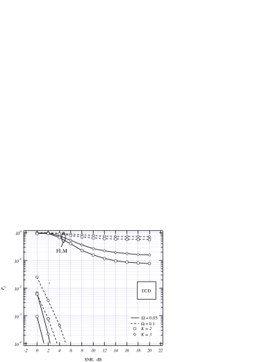
Fig. 1: $P_{f}$ vs. SNR for $K$ = 3 when $\Omega$ is 0.05 or 0.1.

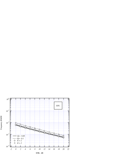
Fig. 2: RMSE vs. SNR for $K$ = 2 or 3 when $\Omega$ is 0.05 or 0.1.

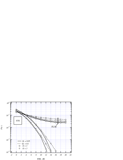
Fig. 3: $P(\epsilon)$ vs. SNR for $K$ = 2 or 3 when $\Omega$ is 0.05 or 0.1.

We begin by investigating the performance of ECD in terms of probability of making an incorrect detection, say $P_{f}$. Fig. 1 illustrates $P_{f}$ as a function of $\mathrm{SNR}=1/\sigma_{n}^{2}$. The number of active RSSs is 3 while the maximum CFO is either $\Omega=0.05$ or 0.1. Comparisons are made with the ranging scheme proposed by Fu, Li and Minn (FLM) in [5]. The results of Fig. 1 indicate that ECD performs remarkably better than FLM.

Fig. 2 illustrates the root mean-square error (RMSE) of the frequency estimates obtained with EFE vs. SNR for $K=2$ or 3 and $\Omega=0.05$ or 0.1. We see that the accuracy of EFE is satisfactory at SNR values of practical interest. Moreover, EFE has virtually the same performance as $K$ or $\Omega$ increase.

The performance of the timing estimators is measured in terms of probability of making a timing error, say $P(\epsilon)$, as defined in [8]. An error event is declared to occur whenever the estimate $\hat{\theta}_{k}$ gives rise to IBI during the data section of the frame. This is tantamount to saying that the timing error $\hat{\theta}_{k}-\theta_{k}+(-N_{G,D}+L)/2$ is larger than zero or smaller than $-N_{G,D}+L-1$, where $N_{G,D}$ is the CP length during the data transmission phase. In the sequel, we set $N_{G,D}=32$. Fig. 3 illustrates $P(\epsilon)$ vs. SNR as obtained with ETE and FLM. The number of active codes is $K=2$ or 3 while $\Omega=0.05$ or 0.1. We see that ETE provides much better results than FLM.

5 Conclusions

We have presented a new ranging method for OFDMA systems in which uplink signals arriving at the BS are impaired by frequency errors in addition to timing misalignments. The synchronization parameters of all ranging users are estimated with affordable complexity through an ESPRIT-based approach. Compared to previous works, the proposed scheme exhibits increased robustness against residual frequency errors and can cope with situations where the CFOs are as large as 10% of the subcarrier spacing.

References

- [1] J. Krinock, M. Singh, M. Paff, A. Lonkar, L. Fung, and C.-C. Lee, “Comments on OFDMA ranging scheme described in IEEE 802.16ab-01/01r1,” Tech. Rep., IEEE 802.16 Broadband Wireless Access Working Group, July 2001.
- [2] X. Fu and H. Minn, “Initial uplink synchronization and power control (ranging process) for OFDMA systems,” in Proceedings of the IEEE Global Communications Conference (GLOBECOM), Dallas, Texas, USA, Nov. 29 - Dec. 3, 2004, pp. 3999 – 4003.
- [3] H. A. Mahmoud, H. Arslan, and M. K. Ozdemir, “Initial ranging for WiMAX (802.16e) OFDMA,” in Proceedings of the IEEE Military Communications Conference, Washington, D.C., October 23-25, 2006, pp. 1 – 7.
- [4] Y. Zhou, Z. Zhang, and X. Zhou, “OFDMA initial ranging for IEEE 802.16e based on time-domain and frequency-domain approaches,” in Proceedings of the International Conference on Communication Technology (ICCT), Guilin, China, November 27-30, 2006, pp. 1 – 5.
- [5] X. Fu, Y. Li, and Hlaing Minn, “A new ranging method for OFDMA systems,” IEEE Transactions on Wireless Communications, vol. 6, no. 2, pp. 659 – 669, February 2007.
- [6] M. Wax and T. Kailath, “Detection of signals by information theoretic criteria,” IEEE Trans.actions on acoustic, Speech and Signal Processing, vol. ASSP-33, pp. 387 – 392, April 1985.
- [7] R. Roy, A. Paulraj, and T. Kailath, “ESPRIT - direction-of-arrival estimation by subspace rotation methods,” IEEE Transactions on Acoustic, Speech and Signal Processing, vol. 37, no. 7, pp. 984 – 995, July 1989.
- [8] M. Morelli, “Timing and frequency synchronization for the uplink of an OFDMA system,” IEEE Transactions on Communications, vol. 52, no. 2, pp. 296 – 306, Feb. 2004.