QCD radiative correction to pair-annihilation of spin-1 bosonic Dark Matter

Abstract

The next-to-leading order (NLO) QCD corrections are calculated for the pair-annihilation of spin-1 dark matter (DM) by dimensionally regularizing both ultraviolet and infrared singularities in non-relativistic limit ($v\ll 1$). The complete $O(\alpha_{s})$ correction is about $8\%$ due to the massless gluon contribution. An extra $5\%$ will be added if there is a new interaction from a massive gluon of approximately same mass as the DM particle. The NLO QCD correction could give the sizable shift to the DM mass constrained by relic density measurements.

I Introduction

The spin-1 dark matter candidate $B^{\prime}$, which is the $Z_{2}$-odd partner of the hypercharge gauge boson $B$, appears in interesting models like universal extra dimensions (UED) tappel and Little Higgs (LH) narkani , motivated by solving the gauge hierarchy problem. The phenomenology of spin-1 DM ($B^{\prime}$) has been well studied at the tree level. With advances in precision measurements in cosmology and astrophysics as well as the advent of LHC era, the NLO calculation of the $B^{\prime}B^{\prime}$ annihilation becomes timely for accurate analysis. We present the next-to-leading order (NLO) QCD corrections for the pair-annihilation of spin-1 bosonic dark matter by dimensionally regularizing both ultraviolet (UV) and infrared (IR) singularities in the non-relativistic limit ($v\ll 1$). Our analysis of the process ($B^{\prime}B^{\prime}\rightarrow q\overline{q}$) is applicable to general spin-1 DM, as in UED, LH, etc. We assume that the quark field $q$ interacts with its $Z_{2}$-odd partner $\widetilde{q}$ in the form.

$$\mathcal{L}\supset-g_{Y}\overline{\widetilde{q}}\gamma^{\mu}(\widetilde{Y}_{L}P_{L}+\widetilde{Y}_{R}P_{R})qB_{\mu}^{\prime}+h.c.$$ (1)

The coupling $g_{Y}$ and the number $\widetilde{Y}_{L}$ in the UED would be the usual hypercharge coupling and the corresponding quantum number,

$$g_{Y}=\frac{e}{\cos\theta_{W}},\text{ \ }\widetilde{Y}_{L}(u,d)=\frac{1}{6},\text{ \ }\widetilde{Y}_{R}(u)=\frac{2}{3},\text{ \ }\widetilde{Y}_{R}(d)=-\frac{1}{3}$$

However in the Littlest Higgs model (L²H) narkani , $\widetilde{Y}_{L}(u,d)=\frac{1}{10}$ and otherwise $\widetilde{Y}_{R}=0$.

We also assume that the mass $\widetilde{M}$ of $\widetilde{q}$ is not too far above the mass $M$ of the spin-1 DM particle $B^{\prime}$. The approximate relation $\widetilde{M}\approx M$ is valid in UED, but a choice of parameters in other models is required. However, such a choice allows us to carry through analytical calculation and give simple results.

Fig.1 shows the Born diagrams for $B^{\prime}(p_{1})B^{\prime}(p_{1}^{\prime})\rightarrow q(p_{2})\overline{q}(p_{2}^{\prime})$. The exchange of the $Z_{2}$-odd quark line is bold-faced. The amplitude for the Born diagrams is given by

$$\mathcal{M}_{B}=-g_{Y}^{2}\widetilde{Y}_{L}^{2}\overline{u}(p_{2})\left(\gamma^{\mu}\frac{{\not p}_{2}-{\not p}_{1}+\widetilde{M}}{t-\widetilde{M}^{2}}\gamma^{\nu}+\gamma^{\nu}\frac{{\not p}_{2}-{\not p}_{1}^{\prime}+\widetilde{M}}{u-\widetilde{M}^{2}}\gamma^{\mu}\right)P_{L}v(p_{2}^{\prime})\epsilon_{\mu}(p_{1})\epsilon_{\nu}(p_{1}^{\prime})\text{\ }+\text{RH}$$ (2)

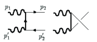
Figure 1: The Born diagrams for $B^{\prime}B^{\prime}\rightarrow q\overline{q}$. The bold wavy lines represent the DM candidate gauge bosons ($B^{\prime}$), the bold solid lines represent the heavy quarks (the $Z_{2}$-odd partners of the outgoing quarks) and the light solid lines correspond to the quarks.

In the extremely non-relativistic limit ($v\simeq 0$), $p_{1}\simeq p_{1}^{\prime}\simeq(p_{2}+p_{2}^{\prime})/2\simeq(M,\mathbf{0})$.  The invariant Mandelstam parameters are

$$s =(p_{1}+p_{1}^{\prime})^{2}=(p_{2}+p_{2}^{\prime})^{2}\simeq 4M^{2}$$ (3a)

$$t =(-p_{1}+p_{2})^{2}=(p_{1}^{\prime}-p_{2}^{\prime})^{2}\simeq-M^{2}$$ (3b)

$$u =(-p_{1}^{\prime}+p_{2})^{2}=(p_{1}-p_{2}^{\prime})^{2}\simeq-M^{2}$$ (3c)

The formula reduces to

$$\mathcal{M}_{B}=g_{Y}^{2}\widetilde{Y}_{L}^{2}\overline{u}(p_{2})\frac{({p}_{2}-{p}_{2}^{\prime})^{\mu}\gamma^{\nu}+({p}_{2}-{p}_{2}^{\prime})^{\nu}\gamma^{\mu}}{M^{2}+\widetilde{M}^{2}}P_{L}v(p_{2}^{\prime})\epsilon_{\mu}(p_{1})\epsilon_{\nu}(p_{1}^{\prime})\ +\text{RH}$$ (4)

The consistent annihilation rate in $d=4-2\epsilon$ dimensions is

$$\sigma_{B}v=\frac{(1-\epsilon)\Gamma(1-\epsilon)}{\Gamma(2-2\epsilon)}\left(\frac{4\pi\mu^{2}}{4M^{2}}\right)^{\epsilon}\frac{2g_{Y}^{4}(\widetilde{Y}_{L}^{4}+\widetilde{Y}_{R}^{4})N_{c}}{9\pi}\frac{M^{2}}{\left(M^{2}+\widetilde{M}^{2}\right)^{2}}$$ (5)

where $N_{c}$ is number of colors, $v$ denotes the relative velocity between spin-1 dark matter candidate pair, $\mu$ is an arbitrary mass scale and $\sigma_{B}$ is the Born cross section.

II Next-to-leading order calculation

The one-loop amplitudes consist of the virtual corrections from the diagrams (a),(b),(c),(d) of Fig.2. Adding up those contributions must be ultraviolet finite. The amplitudes contain infrared divergences due to massless gluon virtual exchange. The infrared should cancel exactly against the one present in the gluon final state radiation, Fig.3(a),(b),(c). The method is to use dimensional regularization in $d=4-2\epsilon$ dimensions with massless on-shell quarks to regularize both types of divergences, UV and IR divergences. The individual diagrams are calculated in the renormalizable Feynman gauge (the gauge parameter, $\xi=1$), which provides the gluon propagator.  All new particles involved in the calculation are set up to have the same mass as $B^{\prime}$.

II.1 Virtual corrections

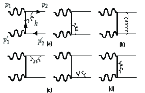
Figure 2: The Feynman diagrams which contribute to the next-to-leading order (NLO) QCD virtual radiative correction($B^{\prime}B^{\prime}\rightarrow q\overline{q}$). The crossed ($u-$channel) diagrams are not displayed. The bold wavy lines represent the DM candidate gauge bosons ($B^{\prime}$), the bold solid lines represent the heavy quarks (the $Z_{2}$-odd partners of the outgoing quarks), curly lines represent the gluons and the light solid lines correspond to the quarks.

All the virtual corrections could be expressed by two form factors related to tensors, $({p}_{2}-{p}_{2}^{\prime})^{\mu}\gamma^{\nu}+({p}_{2}-{p}_{2}^{\prime})^{\nu}\gamma^{\mu}$ and $({p}_{2}+{p}_{2}^{\prime})^{\mu}\gamma^{\nu}+({p}_{2}+{p}_{2}^{\prime})^{\nu}\gamma^{\mu}$, for the massless outgoing particles in static limit. However $({p}_{2}-{p}_{2}^{\prime})^{\mu}\gamma^{\nu}+({p}_{2}-{p}_{2}^{\prime})^{\nu}\gamma^{\mu}$ only survives. ${p}_{2}+{p}_{2}^{\prime}$ is a timelike vector and $B^{\prime}$ polarization vectors, $\epsilon_{\mu}(p_{1})$ and $\epsilon_{\nu}(p_{1}^{\prime})$, are spacelike. The tensor $({p}_{2}+{p}_{2}^{\prime})^{\mu}\gamma^{\nu}+({p}_{2}+{p}_{2}^{\prime})^{\nu}\gamma^{\mu}$ disappears as contracting the $B^{\prime}$ polarization vectors. So the virtual corrections are expressed with only one form factor, which is the coefficient of the Born amplitude.

$$\mathcal{M}_{1}=F_{B^{\prime}}\mathcal{M}_{B}$$ (6)

We use the conventional approach of Feynman parameters to calculate the corrections. The virtual corrections are simplified in the common integral with the shifted momentum and Feynman parameters. The infrared divergences appear in the Feynman parameter integrations.

$$\int\frac{d^{d}\ell dx_{i}}{(2\pi)^{d}}\delta({\textstyle\sum}x_{i}-1)\frac{(\ell^{2})^{r}}{(\ell^{2}-C)^{m}}=\frac{i(-1)^{r-m}}{(4\pi)^{d/2}}\frac{\Gamma(r+d/2)\Gamma(m-r-d/2)}{\Gamma(d/2)\Gamma(m)}\int dx_{i}\delta\left({\textstyle\sum}x_{i}-1\right)C^{r-m+d/2}$$ (7)

The amplitude of the diagrams in Fig.2(a) is

$$\mathcal{M}_{1,L}^{(a)}=-g_{Y}^{2}\widetilde{Y}_{L}^{2}\overline{u}(p_{2})\left[\Gamma_{(a)}^{\mu}\left(\frac{{\not p}_{2}-{\not p}_{1}+M}{t-M^{2}}\right)\gamma^{\nu}+\gamma^{\mu}\left(\frac{{\not p}_{2}-{\not p}_{1}+M}{t-M^{2}}\right)\widetilde{\Gamma}_{(a)}^{\nu}+\mu\leftrightarrow\nu\right]P_{L}v(p_{2}^{\prime})\epsilon_{\mu}(p_{1})\epsilon_{\nu}(p_{1}^{\prime})$$ (8)

$\Gamma_{(a)}^{\mu}$ and $\widetilde{\Gamma}_{(a)}^{\nu}$ are the vertex corrections in $d-$dimensions, which are given by

$$\Gamma_{(a)}^{\mu} =-ig_{s}^{2}C_{F}{\displaystyle\int}\frac{d^{d}k}{(2\pi)^{d}}\frac{\gamma^{\rho}({\not p_{2}}+{\not k})\gamma^{\mu}({\not p_{2}-\not p_{1}}+{\not k}+M)\gamma_{\rho}}{k^{2}(p_{2}+k)^{2}\left((p_{2}-p_{1}+k)^{2}-M^{2}\right)}$$ (9a)

$$\widetilde{\Gamma}_{(a)}^{\nu} =-ig_{s}^{2}C_{F}{\displaystyle\int}\frac{d^{d}k}{(2\pi)^{d}}\frac{\gamma^{\rho}({\not p}^{\prime}{{}_{1}-\not p_{2}}+{\not k}+M)\gamma^{\nu}(-{\not p}^{\prime}{{}_{2}}+{\not k})\gamma_{\rho}}{k^{2}(-p_{2}^{\prime}+k)^{2}\left((p_{1}^{\prime}-p_{2}^{\prime}+k)^{2}-M^{2}\right)}$$ (9b)

where $$g_{s} C_{F} \mu \nu u- t u p_{1} p_{1}^{\prime}, v\simeq 0$$ is the strong coupling and is the Casmir operator of the fundamental representation in the color group. The Lorentz indices and are just switched for the channel, since the invariant Mandelstam parameters and are identical and the momenta, and are timelike in the extremely non-relativistic case().

The form factor of Fig.2(a) results in

$$F_{B^{\prime}}^{(a)}=\frac{\alpha_{s}C_{F}}{2\pi}\left(\frac{4\pi\mu^{2}}{4M^{2}}\right)^{\epsilon}\Gamma(1+\epsilon)\left(\frac{1}{\epsilon_{UV}}+1+\log 2\right)$$ (10)

where the subscript UV implies the $1/\epsilon$ pole coming from UV divergence and $\alpha_{s}(=g_{s}^{2}/4\pi)$ is QCD fine structure constant.

Calculation of Fig.2(b) requires careful and tedious effort because of four propagators in the loop and a three folded integral over Feynman parameters. The scattering amplitude is

$$\mathcal{M}_{1,L}^{(b)}=-g_{Y}^{2}\widetilde{Y}_{L}^{2}\overline{u}(p_{2})\Gamma_{(b)}^{\mu\nu}P_{L}v(p_{2}^{\prime})\epsilon_{\mu}(p_{1})\epsilon_{\nu}(p_{1}^{\prime})$$ (11)

$\Gamma_{(b)}^{\mu\nu}$ is the combined vertex correction of the $t-$ and $u-$channel diagrams. It is given by

$$\Gamma_{(b)}^{\mu\nu}=-ig_{s}^{2}C_{F}\int\frac{d^{d}k}{(2\pi)^{d}}\frac{\gamma^{\rho}({\not p}_{2}+{\not k)}\gamma^{\mu}({\not p_{2}-\not p_{1}}+{\not k+M)}\gamma^{\nu}(-{\not p}_{2}^{\prime}+{\not k)}\gamma_{\rho}+\mu\longleftrightarrow\nu}{k^{2}(p_{2}+k)^{2}(-p_{2}^{\prime}+k)^{2}((p_{2}-p_{1}+k)^{2}-M^{2})}$$ (12)

This integration could also be manipulated into the common form, Eq.(7), however the integral has singularity in the euclidean region. The imaginary parts are included to continue this integral in the euclidean region for the positive $s$ and it results in a complex form factor.

$$F_{B^{\prime}}^{(b)}=\frac{\alpha_{s}C_{F}}{2\pi}\left(\frac{4\pi\mu^{2}}{4M^{2}}\right)^{\epsilon}\Gamma(1+\epsilon)\left(-\frac{1}{\epsilon_{IR}^{2}}-\frac{2}{\epsilon_{IR}}-\frac{14}{3}+\frac{2}{3}\log 2+\frac{2\pi^{2}}{3}+i\pi\left(\frac{1}{\epsilon_{IR}}+3+\frac{\pi}{6}\right)\right)$$ (13)

The imaginary parts are not relevant for real radiative meseurements as a consequence of the unitarity of the $S$-matrix:$S^{{\dagger}}S=1$.

The contribution of Fig.2(c) comes from propagator corrections to on-shell quark lines. For the massless quark lines, there is no contribution using dimensional regularization since the same regulator is used. In the leading order of $\epsilon$, it can be written as

$$F_{B^{\prime}}^{(c)}=\frac{\alpha_{s}C_{F}}{2\pi}\left(\frac{4\pi\mu^{2}}{4M^{2}}\right)^{\epsilon}\Gamma(1+\epsilon)\left(-\frac{1}{2\epsilon_{UV}}+\frac{1}{2\epsilon_{IR}}\right)$$ (14)

However the contribution of Fig.2(d) comes from off-shell heavy quark lines. It produces a contribution without IR divergence.

$$F_{B^{\prime}}^{(d)}=2\frac{d\Sigma_{2}}{d{\not p}}|_{p^{2}=-M^{2}}=\frac{\alpha_{s}C_{F}}{2\pi}\left(\frac{4\pi\mu^{2}}{4M^{2}}\right)^{\epsilon}\Gamma(1+\epsilon)\left(-\frac{1}{2\epsilon_{UV}}-1+\log 2\right)$$ (15)

where the factor of 2 comes from the two vertices and those give identical contributions. The results show that UV divergences are exactly canceled.

Adding up all the virtual corrections, the QCD corrections are

$$\delta_{QCD}^{(\operatorname*{virutal})}=2\operatorname{Re}(F_{B^{\prime}})=\frac{\alpha_{s}C_{F}}{\pi}\left(\frac{4\pi\mu^{2}}{4M^{2}}\right)^{\epsilon}\Gamma(1+\epsilon)\left(-\frac{1}{\epsilon_{IR}^{2}}-\frac{3}{2\epsilon_{IR}}+\frac{2\pi^{2}}{3}-\frac{14}{3}+\frac{8}{3}\log 2\right)$$ (16)

II.2
Real corrections

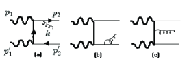
Figure 3: The Feynman diagrams which contribute to the next-to-leading order (NLO) QCD real radiative correction($B^{\prime}B^{\prime}\rightarrow gq\overline{q}$). The crossed ($u-$channel) diagrams are not displayed. The bold wavy lines represent the DM candidate gauge bosons ($B^{\prime}$), the bold solid lines represent the heavy quarks (the $Z_{2}$-odd partners of the outgoing quarks), curly lines represent the gluons and the light solid lines correspond to the quarks.

The real QCD correction appears in the ratio of annihilation rates for two and three body final states. In an average over the polarization of the incoming vector bosons and a sum over the spin and color of outgoing quarks and gluon, the annihilation rate for three body final states is

$$\sigma v=\frac{1}{4M^{2}}\cdot\frac{N_{C}}{9}{\textstyle\int}d\Phi_{3}|\mathcal{M}_{a}+\mathcal{M}_{b}+\mathcal{M}_{c}|^{2}$$ (17)

$\mathcal{M}_{a},\mathcal{M}_{b}$ and $\mathcal{M}_{c}$ are the scattering amplitudes corresponded to the diagrams (a),(b),(c) of Fig.3, and are given by

$$\mathcal{M}_{a,L} =-ig_{Y}^{2}g_{s}\widetilde{Y}_{L}^{2}T^{a}\frac{\overline{u}(p_{2})\gamma^{\rho}({\not p}_{2}+{\not k})\left(\gamma^{\mu}{\not p}_{a}\gamma^{\nu}+\gamma^{\nu}{\not p}_{a}\gamma^{\mu}\right)P_{L}v(p_{2}^{\prime})\epsilon_{\mu}(p_{1})\epsilon_{\nu}(p_{1}^{\prime})\epsilon_{\rho}^{\ast a}(k)}{(p_{2}+k)^{2}(p_{a}^{2}-M^{2})}$$ (18a)

$$\text{\ }\mathcal{M}_{b,L} =-ig_{Y}^{2}g_{s}\widetilde{Y}_{L}^{2}T^{a}\frac{\overline{u}(p_{2})\left(\gamma^{\mu}{\not p}_{b}\gamma^{\nu}+\gamma^{\nu}{\not p}_{b}\gamma^{\mu}\right)(-{\not p}_{2}^{\prime}-{\not k})\gamma^{\rho}P_{L}v(p_{2}^{\prime})\epsilon_{\mu}(p_{1})\epsilon_{\nu}(p_{1}^{\prime})\epsilon_{\rho}^{\ast a}(k)}{(-p_{2}^{\prime}-k)^{2}(p_{b}^{2}-M^{2})}$$ (18b)

$$\mathcal{M}_{c,L} =-ig_{Y}^{2}g_{s}\widetilde{Y}_{L}^{2}T^{a}\frac{\overline{u}(p_{2})\left[\gamma^{\mu}{\not p}_{b}\gamma^{\rho}{\not p}_{a}\gamma^{\nu}+M^{2}\gamma^{\mu}\gamma^{\rho}\gamma^{\nu}+\mu\leftrightarrow\nu\right]P_{L}v(p_{2}^{\prime})\epsilon_{\mu}(p_{1})\epsilon_{\nu}(p_{1}^{\prime})\epsilon_{\rho}^{\ast a}(k)}{(p_{a}^{2}-M^{2})(p_{b}^{2}-M^{2})}$$ (18c)

where $$T^{a} p_{a}=p_{1}^{\prime}-p_{2}^{\prime}=-p_{1}+p_{2}+k,p_{b}=-p_{1}+p_{2}=p_{1}^{\prime}-p_{2}^{\prime}-k p_{1} p_{1}^{\prime} p_{2} p_{2}^{\prime} k$$ is the QCD generator and in shorthand where and are momenta of the incoming vector bosons, and for the outgoing quarks and for the radiated gluon.

$p_{1}\simeq p_{1}^{\prime}\simeq(p_{2}+p_{2}^{\prime}+k)/2\simeq(M,\mathbf{0})$ in the non-relativistic limit and the numerator of $\mathcal{M}_{c}$ is allowed to express by the momenta, $p=p_{2}-p_{2}^{\prime}$ and $k$ on the diagrammetic symmetry.

$$\mathcal{N}_{c}\sim p^{\rho}(p^{\mu}\gamma^{\nu}+p^{\nu}\gamma^{\mu})+ip_{\sigma}k_{\delta}\gamma^{5}\epsilon^{\sigma\rho\delta\lambda}(g_{\lambda}^{\mu}\gamma^{\nu}+g_{\lambda}^{\nu}\gamma^{\mu}-g^{\mu\nu}\gamma_{\lambda})+(p_{2}\cdot p_{2}^{\prime}+2M^{2})(g^{\mu\rho}\gamma^{\nu}+g^{\nu\rho}\gamma^{\mu}-g^{\mu\nu}\gamma^{\rho})$$ (19)

The relation, $\epsilon_{\rho}(p)\epsilon_{\sigma}^{\ast}(p^{\prime})=-g_{\rho\sigma}$, is adopted to calculate the squared amplitude for both incoming massive spin-1 dark matter candidates in Feynman gauge, since the polarization vectors $\epsilon_{\mu}(p_{1}),\epsilon_{\nu}(p_{1}^{\prime})$ are spacelike. The soft and collinear singularities appear in the squared amplitudes, $|$$\mathcal{M}_{a}|^{2},$$|$$\mathcal{M}_{b}|^{2}$ and $2\operatorname{Re}(\mathcal{M}_{a}^{\ast}\mathcal{M}_{b})$. $1/\epsilon$ poles are canceled out in 2$\operatorname{Re}(\mathcal{M}_{a}^{\ast}\mathcal{M}_{c})$ and 2$\operatorname{Re}(\mathcal{M}_{b}^{\ast}\mathcal{M}_{c})$ as combining the numerator and denominator, and $\left|\mathcal{M}_{c}\right|^{2}$ is totally free of IR divergences.

The new dimensionless parameters are introduced for the phase space integration by energy-momentum conservation.

$$x_{1}=\frac{p_{2}\cdot k}{2M^{2}},\qquad x_{2}=\frac{p_{2}^{\prime}\cdot k}{2M^{2}},\qquad x_{3}=\frac{p_{2}\cdot p_{2}^{\prime}}{2M^{2}}$$ (20)

$1/\epsilon$ poles appear at $x_{1}=0$ and $x_{2}=0.$ The Lorentz-invariant three body phase space takes the form with the new parameters.

$${\textstyle\int}d\Phi_{3}=\frac{4M^{2}}{(4\pi)^{3}\Gamma(2-2\epsilon)}\left(\frac{4\pi\mu^{2}}{4M^{2}}\right)^{2\epsilon}{\textstyle\int}dx_{1}dx_{2}dx_{3}(x_{1}x_{2}x_{3})^{-\epsilon}\delta({\textstyle\sum}x_{i}-1)$$ (21)

The overall real correction gives

$$\delta_{QCD}^{(\operatorname{real})}=\frac{\alpha_{s}C_{F}}{\pi}\left(\frac{4\pi\mu^{2}}{4M^{2}}\right)^{\epsilon}\Gamma(1+\epsilon)\left(\frac{1}{\epsilon_{IR}^{2}}+\frac{3}{2\epsilon_{IR}}+\frac{39}{4}-\frac{7}{6}\pi^{2}\right)$$ (22)

When all the contributions are added, the infrared are exactly canceled and the finite result is

$$\delta_{QCD}=\frac{\alpha_{s}C_{F}}{\pi}\left(\frac{61}{12}+\frac{8}{3}\log 2-\frac{\pi^{2}}{2}\right)\text{ }$$ (23)

The correction is about 8$\%$ enhancement for $C_{F}=4/3$ and $\alpha_{s}($1TeV$)=0.09$, and the finiteness of this correction implies that there is no divergence by degeneracy.

II.3 The corrections by the heavy gluon

If the heavy $Z_{2}$-odd of the usual gluon is not far above $M$, its contribution to the $B^{\prime}$ pair annihilation could be important. The relevant Lagrangian of this heavy gluon field $G_{\mu}^{\prime a}$ is

$$\mathcal{L}\supset-g_{s}\overline{\widetilde{q}}\gamma^{\mu}T^{a}G_{\mu}^{{}^{\prime}a}q+h.c.$$ (24)

For being able to carry through analytical calculation, we set the mass of this heavy gluon field $G_{\mu}^{\prime a}$ equal to the $B^{\prime}$ mass $M$ in our calculation. Such a simplification is valid at least in UED. The corresponding Feynman diagrams are similarly given in Fig. 2, except that we need to interchange the bold quark line and the light quark line in the loop as well as the usual gluon is replaced by the heavy gluon. Note that there is no IR divergence for a massive gluon, and the UV divergence cancels among diagrams. As a single heavy gluon cannot be produced by $Z_{2}$-symmetry, the diagrams in Fig. 3 are all absent and it results in the improved QCD correction. The QCD corrections by the heavy gluon can also be calculated fully analytically and the overall correction is

$$\delta_{QCD}^{(\operatorname*{gluon})}=\frac{\alpha_{s}C_{F}}{\pi}\left(-5+\frac{9\pi^{2}}{8}-10\log 2+\frac{7\pi}{6\sqrt{3}}\right)\text{ }$$ (25)

The correction is about $5\%$ enhancement and is comparable to massless gluon correction.

III Application to relic abundance

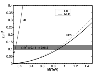
Figure 4: Prediction for relic abundance as a function of the WIMP mass. NLO QCD radiative corrections are considered on the solid lines. The horizonal band denotes $\Omega$h²=0.111$\pm$0.012 and defines the WIMP mass window. The WIMP mass in the window is shifted about 50 GeV for UED with NLO QCD correction.

The spin-1 dark matter candidate $B^{\prime}$, which is the $Z_{2}$-odd partner of the hypercharge gauge boson $B$, has been an attractive dark matter candidate in UED and LH, but both models were extended in different ways. The spatial dimensions are enlarged for UED, otherwise the symmetry groups are enlarged for LH in 4-dimensions. So the masses of the new particles are scaled by the extra dimension of size $R$ compactified on an $S^{1}/Z_{2}$ orbifold for UED and the enlarged global symmetry breaking scale $f$  for LH. Since the new particles are in the different symmetry group structure, the different gauge charges are assigned to the fermions ($q\widetilde{q}B^{\prime}$ coupling) and it causes them to induce the different phenomenological analyses. We consider relic abundance with our QCD correction, but the detailed analyses are not mentioned since those were well studied in the leading order in the other articlesgeraldine ; andreas .

Assuming that the spin-1 $B^{\prime}$ accounts for all DM relic abundance, one can constrain its mass $M$ based on the pair annihilation rate in the early universe. In UED models, the annihilation channel into a fermion pair $B^{\prime}B^{\prime}\rightarrow f\overline{f}$ dominates because of sizable couplings of the gauge charges $\widetilde{Y}_{L/R}$. The measured relic abundance prefers $M$ to be about TeV. On the contrary, the L²H model has rather small couplings of the gauge charges $\widetilde{Y}_{L}=\frac{1}{10}$,$\widetilde{Y}_{R}=0$, and the relic abundance only requires $M$ of order of 100 GeV. The detailed quantitative analyses for relic abundance by this type of WIMP annihilations can be found in Ref.geraldine for UED and Ref.andreas for LH. Fig.4 shows the prediction for relic abundance as a function of WIMP mass with the present WMAP precision dnspergel . The WIMP mass in the window is shifted about 50 GeV compared to the leading order for UED, but it shows no difference from the leading order by the negligible annihilation fractions into quarks for LH .

IV Conclusion

The next-to-leading order (NLO) QCD corrections are calculated for pair-annihilation of spin-1 bosonic dark matter by dimensionally regularizing both ultraviolet and infrared singularities in the non-relativistic limit. The order $\alpha_{s}$ correction amounts to about $8\%$ and can enhance to $13\%,$ when including heavy gluon. The NLO QCD correction could give the sizable shift to the DM mass constrained by relic density measurements.

*

Appendix A Useful formulas and identities

The Dirac algebra in $d=4-2\epsilon$ dimensions are listed in Ref.wjmar and they could be induced by the anticommutator $\left\{\gamma^{\mu},\gamma^{\nu}\right\}=2g^{\mu\nu}$ and the identity $\gamma^{\mu}\gamma_{\mu}=d$. The regulator $\epsilon$ is omitted on trace algebra Tr$\left[\text{I}\right]=2^{d/2}$ for two and three body cross section calculations.

$1/\epsilon_{IR}$ poles are extracted by the partial integrations on the loop calculations in case of a need to extract the poles and the remnants are expanded in ordinary Taylor series with respect to $\epsilon$. The three folded parametric integrals for the box diagram are calculated by Feynman parameter properties, since one of them is not symmetric with the others.

$$\int_{0}^{1}dx\int_{0}^{1-x}dyf(x,y)=\int_{0}^{1}dy\int_{0}^{1-y}dxf(x,y)$$ (26)

The complicated integrations are avoided and number of integrations is reduced with this property.

The useful identity to split the singular and non-singular parts for the real corrections is

$$\frac{1}{x(1-x)}=\frac{1}{x}+\frac{1}{1-x}$$ (27)

This identity can be extended to the higher powers of the variables and will simplify the calculations since the regulator $\epsilon$ can be dropped for non-singular parts.

Some of the parametric integrals contain the dilogarithm (or spence) function.

$$\text{Li}_{2}(x)\equiv-\int_{0}^{1}dt\frac{\log(1-xt)}{t}$$ (28)

The values which appear in our calculations are

$$\text{Li}_{2}(1) =\frac{\pi^{2}}{6}\text{ }$$ (29a)

$$\text{\ Li}_{2}(-1) =-\frac{\pi^{2}}{12}\text{ }$$ (29b)

$$\text{\ Li}_{2}\left(\frac{1}{2}\right) =\frac{\pi^{2}}{12}-\frac{\log^{2}2}{2}$$ (29c)

The parametric integrals which appeared in the box diagrams reduce to the incomplete beta function.

$$B_{1/2}(m,n)\equiv\int_{0}^{1/2}dxx^{m-1}\left(1-x\right)^{n-1}$$ (30)

$$B_{1/2}(m,n)+B_{1/2}(n,m) =B(m,n)$$ (31a)

$$B_{1/2}(m,m) =\frac{1}{2}B(m,m)$$ (31b)

$$B_{1/2}(m,m+1) =\frac{1}{2}\left[B(m,m+1)+\frac{2^{-2m}}{m}\right]$$ (31c)

$$B_{1/2}(m,m+2) =\frac{1}{2}\left[B(m,m+2)+\frac{2^{-2m}}{m}\right]$$ (31d)

where

$$B(m,n)=\frac{\Gamma(m)\Gamma(n)}{\Gamma(m+n)}$$ (32)

For integer $n$, the Taylor expansion is adopted with respect to $\epsilon$.

$$B_{z}(-\epsilon,0) =1+\epsilon\log(1-z)-\epsilon^{2}\text{Li}_{2}(z)$$ (33a)

$$B_{z}(-\epsilon,1) =1+\epsilon\left(-\frac{z}{1-z}+\log(1-z)\right)+\epsilon^{2}\left(\log(1-z)-\text{Li}_{2}(z)\right)$$ (33b)

with $z=1/2.$

The parametric integrations involved the heavy gluon loops are

$$\int_{0}^{1}dx\log(x^{2}-x+1) =2\left(\frac{\sqrt{3}}{6}\pi-1\right)$$

$$\int_{0}^{1}dx(x^{2}-x)\log(x^{2}-x+1) =\frac{17}{18}-\frac{\sqrt{3}}{6}\pi$$

$$\int_{0}^{1}dx\frac{x^{2}-x}{x^{2}-x+1} =-1+\frac{2}{3\sqrt{3}}\pi$$

References

• (1) T. Appelquist, H. C. Cheng and B. A. Dobrescu, Phys. Rev. D 64, 035002 (2001) [arXiv:hep-ph/0012100]
• (2) N. Arkani-Hamed, A. G. Cohen, E. Katz, and A. E. Nelson, JHEP 07, 034 (2002); H. C. Cheng and I. Low, JHEP 0309, 051 (2003)[arXiv:hep-ph/0308199] ; JHEP 0408, 061 (2004) [arXiv:hep-ph/0405243]; I. Low, JHEP 0410, 067 (2004) [arXiv:hep-ph/0409025]
• (3) K. Hagiwara, C.B. Kim and T. Yoshino, Nuclear Physics B 177, 461 (1981); B. Mele, P. Nason and G. Ridolfi. Nuclear Physics B 357, 409 (1991)
• (4) G. Servant, T. M. P. Tait, Nucl. Phys. B 650, 391 (2003) [arXiv:hep-ph/0206071]; K. Kong and K.T. Matchev, JHEP 0601, 038 [arXiv:hep-ph/0509119]
• (5) Andreas Birkedal, Andrew Noble, Maxim Perelstein, and Andrew Spray, Phys. Rev D 74, 035002 (2006) [arXiv:hep-ph/0603077]
• (6) D. N. Spergel $et$ $al$., [WMAP Collaboration], Astrophys. J Suppl. 170, 377 (2007) [arXiv:astro-ph/0603449]
• (7) W. J. Marciano, Phys. Rev. D 12, 3861 (1975), ”Dimensional regularization is well explained in this letter”