A gradient-directed Monte Carlo approach to molecular design

Abstract

The recently developed linear combination of atomic potentials (LCAP) approach [M. Wang et al., J. Am. Chem. Soc., 128, 3228 (2006)] allows continuous optimization in discrete chemical space and thus is quite useful in the design of molecules for targeted properties. To address further challenges arising from the rugged, continuous property surfaces in the LCAP approach, we develop a gradient-directed Monte Carlo (GDMC) strategy as an augmentation to the original LCAP optimization method. The GDMC method retains the power of exploring molecular space by utilizing local gradient information computed from the LCAP approach to jump between discrete molecular structures. It also allows random Monte Carlo moves to overcome barriers between local optima on property surfaces. The combined GDMC and LCAP approach is demonstrated here for optimizing nonlinear optical (NLO) properties in a class of donor-acceptor substituted benzene and porphyrin frameworks. Specifically, one molecule with four nitrogen atoms in the porphyrin ring was found to have a larger first hyperpolarizability than structures with the conventional porphyrin motif.

I Introduction

Molecular and material design presents an extremely challenging problem because the number of accessible stable candidate molecules in the sampling space is immense(Lipinski and Hopkins, 2004; Ertl, 2003; Dobson, 2004). In such a vast molecular space, direct enumeration and evaluation of molecules are expensive and inefficient. Furthermore, since each molecular structure in the space is unique and discrete, traditional methods are usually based on combinatorial chemistry. Each molecule is generated from building blocks and its specific chemical properties are analyzed for selection in the design process. Thus, a number of discrete optimization approaches, such as branch-and-bound methods(Ostrovsky et al., 2002), Monte Carlo, and genetic algorithms(Wales and Scheraga, 1999; Kuntz et al., 1994; Jorgensen, 2004), have been utilized to explore the rich molecular space for the desired chemical properties. All of these approaches require extensive molecular property computations to obtain some optimal structures. To overcome the difficulties associated with discrete optimization, several approaches(Franceschetti and Zunger, 1999; Kuhn and Beratan, 1996) have been proposed to transform the discrete optimization into a continuous optimization. However, none of these methods can be generalized to optimize the desired properties for molecular design. Recently, we introduced a linear combination of atomic potentials (LCAP) scheme (Wang et al., 2006). The LCAP method provides a smooth chemical property surface interpolating those of the discrete target molecules, thus facilitates property optimization for molecular design. A related approach has also been suggested but was based on atom type variation in a fixed chemical skeleton(von Lilienfeld et al., 2005).

A molecule or solid is characterized by its electron-nuclear potential

$$v(\mathbf{r})=-\sum_{\mathbf{R}}\frac{Z_{\mathbf{R}}}{|\mathbf{r}-\mathbf{R}|}$$ (1)

where $Z_{\mathbf{R}}$ is the atomic number at position $\mathbf{R}$. This electrostatic potential and the number of electrons $N$, enter the Schrödinger equation and determine the properties of the molecules. As such, molecular or material properties are functionals of $v(\mathbf{r})$ and $N$ .

In the LCAP approach, we thus formulate the design of optimized molecules or materials as the optimization of properties in the functional space of $v(\mathbf{r})$ and $N$ (Wang et al., 2006). The advantages of optimization based on the potential arise from both the potential’s “smoothness” and the favorable scaling of the computational cost with system size. The complexity of the potential function grows linearly with the molecular size. This is in stark contrast to the combinatorial explosion of possible molecular structures that would fill a growing molecular volume. The challenge at hand is how best to carry out the potential-function optimization; it is essential that the optimized potential be linked to real molecules. While all molecules lie within the space of all $v(\mathbf{r})$, not all potentials map back to chemical structures. A full optimization in potential space most likely will lead to a potential that does not map to a molecule, which has a limited form of the potential given by eq. (1).

The LCAP method is an effective way to limit the scope of the optimization in potential space. Specifically, the potential is expanded as a linear combination of atomic potentials,

$$v(\mathbf{r})=\sum_{\mathbf{R},A}b_{A}^{\mathbf{R}}v_{A}^{\mathbf{R}}(\mathbf{r})$$ (2)

where $v_{A}^{\mathbf{R}}(\mathbf{r})$ is the potential of an atom (or chemical group) $A$ at position $\mathbf{R}$, $v_{A}^{\mathbf{R}}(\mathbf{r})=\sum_{B}v_{B}(\mathbf{r})$, $v_{B}(\mathbf{r})=-\tfrac{Z_{\mathbf{R}}}{|\mathbf{r}-\mathbf{R}|}$. The coefficient $b_{A}^{\mathbf{R}}$ defines the admixture of a particular atom or group in the molecular potential. The constraints on $b_{A}^{\mathbf{R}}$ are $\sum_{A}b_{A}^{\mathbf{R}}=1$ and $0\leq b_{A}^{\mathbf{R}}\leq 1$. When $b_{A}^{\mathbf{R}}=0$ or $b_{A}^{\mathbf{R}}=1$ for each $\mathbf{R}$, $v(\mathbf{r})$ corresponds to a “real” molecule. Therefore, within the LCAP framework, the design of molecules with an optimized targeted property becomes the optimization of the coefficients $\{b_{A}^{\mathbf{R}}\}$ for given sets of $\mathbf{R}$ (geometry) and $v_{A}^{\mathbf{R}}$ (atom or group types). The LCAP scheme has been used to find the potential function that produces structures with optimal properties, such as electronic polarizabilities and first hyperpolarizabilities for the simple case with two substitution sites. We showed that the optimal structures can be determined without directly enumerating all of the possible structures. We further implemented the LCAP scheme in the tight-binding and semi-empirical frameworks(Xiao et al., 2008; Keinan et al., 2007). Our studies showed that the linear combination of atomic/group coefficients in LCAP indeed smooths out the discreteness of the molecular space and facilitates continuous optimization.

However, when molecular diversity grows (e.g., as chemical groups of varying structure, number of electrons, etc. enter), the ruggedness of the property surfaces grows as well. The rugged surface makes the property optimizations inefficient, since the optimization becomes easily trapped in local minima. In addition, a fractional number of electrons may appear during the continuous optimization process, which can lead to convergence difficulty for the property calculations when using quantum mechanical approaches.

In this paper, we develop an optimization approach, the gradient-directed Monte Carlo (GDMC) approach, which retains the convenience of continuous optimization while circumventing some of the difficulties associated with the ruggedness of property surfaces. The method utilizes local gradient information with respect to the LCAP coefficients $\{b_{A}^{\mathbf{R}}\}$, but preserves the simplicity of exploring molecular space by jumping between discrete molecular structures. It also allows random Monte Carlo jumps to overcome barriers between local property minima. As such, the GDMC method avoids the surface ruggedness that arises from chemical structures of “intermediate” composition (i.e., structures with non-integer LCAP coefficients; see Ref. (Wang et al., 2006) for further information). Note that the application GDMC in conjunction with using finite difference approximation to the gradients was reported in Ref. Keinan et al. (2007), without a description of algorithmic details. The related LCAP application to locate the deepest minimum energy configuration of face centered cubic Au - Pd alloys has also been reported.(d’Avezac and Zunger, 2007) In a related manner, the trial wave function in a fixed-node quantum Monte Carlo method(Reynolds et al., 1982) “serves as a guiding function for a random walk of the electrons through configuration space”, which is indeed a biased MC approach for the continuous electron coordinate space. This is similar with our proposed GDMC approach for the discrete molecular space.

We apply the combined GDMC and LCAP approaches to optimize the static first electronic hyperpolarizability $\beta$ for molecular libraries. In Section II, the LCAP approach for the first hyperpolarizability is explained briefly. In Section III, the general GDMC algorithm is introduced for molecular property optimization. Section IV describes how to combine GDMC with the LCAP method to optimize the first electronic hyperpolarizability. Three examples of hyperpolarizability optimization are presented in Section V. Finally, Section VI summarizes the combined GDMC and LCAP approaches.

II The LCAP approach for the first hyperpolarizability

Traditional molecular design is carried out by examining families of discrete structures, which may be generated using combinatorial libraries, intuition, or qualitative structure-activity relationships. But for any molecule, the Schrödinger equation is determined by the nuclear-electron attraction potential $v(\mathbf{r})$ and the number of electrons $N$. Optimization of $v(\mathbf{r})$, as developed in our recent studies(Wang et al., 2006), is appealing because continuous search algorithms based on gradient calculations can be much more efficient than traditional molecular design methods. The discrete molecular optimization problem becomes a continuous one when $v(\mathbf{r})$ is expanded as a linear combination of atomic potentials (LCAP), as in Eq.( 2).

In this paper, we are interested in the linear and nonlinear response properties to an external electric field. In an electric field $\mathbf{F}$, the molecular energy is

$$E(\mathbf{F}) = E(0)-\sum_{i}\mu_{i}F_{i}-\frac{1}{2!}\sum_{ij}\alpha_{ij}F_{i}F_{j}$$ (3)

$$- \frac{1}{3!}\sum_{ijk}\beta_{ijk}F_{i}F_{j}F_{k}-\frac{1}{4!}\sum_{ijkl}\gamma_{ijkl}F_{i}F_{j}F_{k}F_{l}-\cdots$$

where $E(0)$ is the energy in the absence of the applied electric field, the indices $i$, $j$, $k$, and $l$ span the molecular ($x$, $y$, and $z$) axes, $\mu_{i}$ is the permanent dipole moment and $\alpha_{ij}$ is the (linear) polarizability. The first hyperpolarizability is $\beta_{ijk}$ and the second hyperpolarizability is $\gamma_{ijkl}$. We focus on the static first hyperpolarizability in this paper. Specifically, the first hyperpolarizability tensor element $\beta_{zzz}$ along the z-axis can be calculated using the finite-field approach (Kurtz and Dudis, 1998; Kurtz et al., 1990):

$$\beta_{zzz}=\left[-\frac{1}{2}\left\{E(2F_{z})-E(-2F_{z})\right\}+\left\{E(F_{z})-E(-F_{z})\right\}\right]/F_{z}^{3}$$ (4)

where $F_{z}$ is the applied electric field along the z-axis and $E(F_{z})$ is the corresponding energy.

In the LCAP approach, the $\beta_{zzz}$ gradients with respect to the LCAP coefficients $\{b_{A}^{\mathbf{R}}\}$ are,

$$\frac{\partial\beta_{zzz}}{\partial b_{A}^{\mathbf{R}}} = \left\{-\frac{1}{2}\left[\frac{\partial E(2F_{z})}{\partial b_{A}^{\mathbf{R}}}-\frac{\partial E(-2F_{z})}{\partial b_{A}^{\mathbf{R}}}\right]+\left[\frac{\partial E(F_{z})}{\partial b_{A}^{\mathbf{R}}}-\frac{\partial E(-F_{z})}{\partial b_{A}^{\mathbf{R}}}\right]\right\}/F_{z}^{3}$$ (5)

$$= \left\{-\frac{1}{2}\left[\left.\frac{\partial E(2F_{z})}{\partial b_{A}^{\mathbf{R}}}\right|_{N}-\left.\frac{\partial E(-2F_{z})}{\partial b_{A}^{\mathbf{R}}}\right|_{N}\right]+\left[\left.\frac{\partial E(F_{z})}{\partial b_{A}^{\mathbf{R}}}\right|_{N}-\left.\frac{\partial E(-F_{z})}{\partial b_{A}^{\mathbf{R}}}\right|_{N}\right]\right\}/F_{z}^{3}+$$

$$\left\{-\frac{1}{2}\left[\left.\frac{\partial E(2F_{z})}{\partial b_{A}^{\mathbf{R}}}\right|_{v}-\left.\frac{\partial E(-2F_{z})}{\partial b_{A}^{\mathbf{R}}}\right|_{v}\right]+\left[\left.\frac{\partial E(F_{z})}{\partial b_{A}^{\mathbf{R}}}\right|_{v}-\left.\frac{\partial E(-F_{z})}{\partial b_{A}^{\mathbf{R}}}\right|_{v}\right]\right\}/F_{z}^{3}$$

as implemented(Wang et al., 2006) in the PWSCF(Baroni et al., 2002) program based on plane waves with ultra-soft pseudopotentials (USPP)(Vanderbilt, 1990). In PWSCF, for atom $A$, $v_{A}^{\mathbf{R}}(\mathbf{r})$ is replaced by the USPP,

$$v_{A}(\mathbf{r},\mathbf{r}^{\prime}) = v_{A}^{loc}(\mathbf{r},\mathbf{r}^{\prime})+v_{A}^{nl}(\mathbf{r},\mathbf{r}^{\prime})$$ (6)

$$= v_{A}^{loc}(r)\delta(\mathbf{r}-\mathbf{r}^{\prime})+\sum_{nm}D_{nm}^{0}|\beta_{n}^{A}\left>\right<\beta_{m}^{A}|$$

where $D_{nm}^{0}$, $\beta_{n}^{A}$ and $v_{A}^{loc}(r)$ characterize the USPP for atom $A$. The electrostatic potential $v(\mathbf{r})$ can be expanded as a linear combination of atomic potentials in the USPP framework,

$$v(\mathbf{r},\mathbf{r}^{\prime}) = \sum_{\mathbf{R},A}b_{A}^{\mathbf{R}}v_{A}^{\mathbf{R},loc}(r)\delta(\mathbf{r}-\mathbf{r}^{\prime})+\sum_{\mathbf{R},A}b_{A}^{\mathbf{R}}v_{A}^{\mathbf{R},nl}(\mathbf{r},\mathbf{r}^{\prime})$$ (7)

$$= v^{loc}(\mathbf{r},\mathbf{r}^{\prime})+v^{nl}(\mathbf{r},\mathbf{r}^{\prime})$$

where the first term is the total local potential and the second term is the total nonlocal potential of $v(\mathbf{r})$ for the system. The total energy of the system in an external electric field can then be written

$$E(F_{z}) = \sum_{i}\left<\phi_{i}\left|-\frac{\hbar}{2m}\nabla^{2}+v^{nl}(\mathbf{r},\mathbf{r}^{\prime})\right|\phi_{i}\right>+E_{H}\left[n(\mathbf{r})\right]$$ (8)

$$+ E_{xc}\left[n(\mathbf{r})\right]+\int d\mathbf{r}\left(v^{loc}(\mathbf{r})-zF_{z}\right)n({\mathbf{r}})$$

where

$$n(\mathbf{r}) = \sum_{i}\left[|\phi_{i}|^{2}+\sum_{\mathbf{R},A}b_{A}^{\mathbf{R}}\sum_{nm}Q_{nm}^{A}\left<\phi_{i}|\beta_{n}^{A}\right>\left<\beta_{m}^{A}|\phi_{i}\right>\right]$$ (9)

$$\left<\phi_{i}|S|\phi_{j}\right> = \delta_{ij},S=1+\sum_{\mathbf{R},A}\sum_{nm}b_{A}^{\mathbf{R}}q_{nm}^{A}|\beta_{n}^{A}\left>\right<\beta_{m}^{A}|.$$ (10)

Here, $q_{nm}^{A}=\int d\mathbf{r}Q_{nm}^{A}(\mathbf{r})$. From eqs. 8, 9, 10, the derivative of the total energy with respect to the coefficients $b_{A}^{\mathbf{R}}$ with $N$ electrons is:

$$\frac{\partial E(F)}{\partial b_{A}^{\mathbf{R}}}=\left.\frac{\partial E(F)}{\partial b_{A}^{\mathbf{R}}}\right|_{N}+\left.\frac{\partial E(F)}{\partial b_{A}^{\mathbf{R}}}\right|_{v(\mathbf{r},\mathbf{r}^{\prime})}$$ (11)

where

$$\left.\frac{\partial E(F)}{\partial b_{A}^{\mathbf{R}}}\right|_{N} = \sum_{i}\sum_{nm}D_{nm}^{A}\left<\phi_{i}|\beta_{n}^{A}\right>\left<\beta_{m}^{A}|\phi_{i}\right>+\int v_{A}^{\mathbf{R},loc}(\mathbf{r})n(\mathbf{r})d\mathbf{r}$$ (12)

$$- \sum_{i}\epsilon_{i}\sum_{nm}q_{nm}^{A}\left<\phi_{i}|\beta_{n}^{A}\right>\left<\beta_{m}^{A}|\phi_{i}\right>$$

$$\left.\frac{\partial E(F)}{\partial b_{A}^{\mathbf{R}}}\right|_{v=v(\mathbf{r},\mathbf{r}^{\prime})} = \frac{\partial E(F)}{\partial N}\frac{\partial N}{\partial b_{A}^{\mathbf{R}}}=\mu Z_{A}^{\mathbf{R}}$$ (13)

Here, $D_{nm}^{A}=D_{nm}^{0}+\int V_{eff}(\mathbf{r})Q_{nm}^{A}(\mathbf{r})d\mathbf{r}$, $V_{eff}(\mathbf{r})=V_{H}(\mathbf{r})+V_{xc}(\mathbf{r})+v^{loc}(\mathbf{r})-zF$, and $\sum_{\mathbf{R},A}Z_{A}^{\mathbf{R}}=N$. The chemical potential of the system is $\mu$ , and $Z_{A}^{\mathbf{R}}$ is the atomic number of atom $A$, or the electron number of functional group $A$ at position $\mathbf{R}$. After obtaining the gradients $\{\frac{\partial E}{\partial b_{A}^{\mathbf{R}}}\}$, the $\beta_{zzz}$ gradients with respect to LCAP coefficients can be computed using eq. 5. As described in Ref. (Wang et al., 2006), with the availability of gradients, continuous optimization can be carried out effectively.

Our studies with expanded molecular fragment libraries showed that the property surfaces can become too complicated to permit efficient hyperpolarizability optimization in the continuous space. Indeed, for the specific NLO properties, potentials associated with non-integer LCAP coefficients can have large and rapidly varying hyperpolarizabilities as electron numbers are varied and as electronic states move in and out of degeneracy. This challenge presented by adding richness to the LCAP library suggests that we could modify the optimization method in a way that retains the power and appeal of the LCAP approach while side-stepping the ruggedness associated with the non-integer (not realizable, or “intermediate”) molecular structures. In the following section, we present the development in which the GDMC and LCAP methods are combined to overcome the difficulties associated with the ruggedness of the property surface.

III The general GDMC approach

For a given discrete space, the discrete optimization problem may be transformed into be a continuous one by interpolation (Wang et al., 2006; Koh et al., 2005; Koh and Ananthasuresh, 2005). Then, the interpolated continuous surface can be used for the specific optimization problem of interest. For example, in molecular design, when one fragment $A$ is replaced by another fragment $B$ to form a new molecule, this transformation is indeed discrete. Additionally, the weighting of each fragment at each site is defined by one coefficient. When the molecule contains $A$, the coefficient of $A$ is set to 1; otherwise it is set to 0. The set of coefficients (either 0 or 1) corresponds to one real molecule. Thus, normal integer programming algorithms such as Monte Carlo and genetic algorithms can be applied to search in the discrete space. However, we can also allow $A$ to change continuously to $B$, which means the $A$ coefficient is decreased from 1 to 0 continuously and the $B$ coefficient is increased from 1 to 0. It is then possible to use gradients with respect to the coefficients to aid the molecular property optimization. Mathematically, the LCAP coefficients discussed in Section II play the same roles in the potential optimization to transform a discrete problem into a continuous one. The possible transformations are not unique. Some approaches may simplify the optimization problem while others may worsen the problem, depending on the property and the specific molecular fragment libraries. In the LCAP approach, when the coefficients are between 0 and 1, the system becomes an “intermediate” or alchemical species. It may lead to non-smooth behavior of the molecular property in the unphysical intermediate states. Such a scenario was encountered in the LCAP continuous optimization due to the fractional number of electrons when the NLO properties were targeted for optimization. We have found that the system with one fractional electron is more likely to have a much higher nonlinear polarizability than the corresponding systems with an integer number of electrons because the NLO property is quite sensitive to the electronic states. Thus, it may be particularly ineffective to optimize NLO properties for diverse libraries on an interpolated continuous surface.

Although the interpolated continuous surface may be rugged, the local gradient information for each set of coefficients represents approximately how the property varies when the coefficients change. For example, as demonstrated in our previous studies(Keinan et al., 2007), calculated gradients for the real molecule were used to build the next molecule and to guide the search efficiently. But the search can be easily trapped in local optima. Therefore, we develop a new strategy, the gradient-directed Monte Carlo (GDMC) approach, to deal with the global optimization of discrete variables. GDMC utilizes the local gradients to enhance the search for local optima, while the stochastic jumps overcome the barriers between local optima. The details of a GDMC calculation for the minimization of a general property $P$ consist of the following steps :

1. Set the iteration number $i=0$ and begin with an initial set of coefficients $\{b_{A}^{1}\}$ (either 0 or 1) at each site.

2. Set $i=i+1$. Calculate the property $P_{i}$ and its gradients $\frac{\partial P_{i}}{\partial b_{A}^{i}}$ with respect to all coefficients $\{b_{A}^{i}\}$ at each site. Exit if the optimization goal or the maximum number of iteration is reached.

3. Make a trial move to generate a new set of $\{b_{A}^{i}\}$ following the computed gradients $\{\frac{\partial P_{i}}{\partial b_{A}^{i}}\}$. Accept the trial move with the probability $p=min\{1,\>e^{-\beta(P_{i}-P_{i-1})}\}$ using the Metropolis rule. If the trial move is accepted, go to step 2; If the trial move is rejected, go to step 3 .

Here, $\beta=1/(kT)$. On the energy surface, $k$ is Boltzmann’s constant and $T$ is the temperature. However, on the property surface, $k$ and $T$ are two parameters: the value of $k$ is constant; $T$ is an empirical temperature that controls the probability of accepting a set of coefficients. The rules for generating new trial molecules following the LCAP gradients are described in the next section.

Compared to the classical MC method, GDMC does not randomly vary the coefficients. All of the coefficients (either 0 or 1) that describe the discrete space are generated from the property gradients that can be defined in many ways. As shown in Section IV, we redefined the LCAP gradients associated with GDMC to optimize the NLO properties in three different examples. It is also worth noting that the GDMC approach is suitable for any discrete optimization that possesses a smoothed-out virtual continuous surface.

IV Combining GDMC and LCAP

We use the absolute value of the first hyperpolarizability as the object function in the GDMC optimization. For the LCAP approach, the gradients $\{\frac{\partial\beta_{zzz}}{\partial b_{A}^{\mathbf{R}}}\}$ (eq. 5) include the chemical potential $\mu=\left(\frac{\partial E}{\partial N}\right)_{v}$ (see eq. 13), which has two values for each of the directions of change in the number of electrons and can be calculated based on the formula recently derived for any DFT calculations.(Cohen et al., 2008) Here, we found it possible to bypass the need to calculate $\mu$. We redefine the LCAP gradients by a normalization,

$$\frac{\partial\beta_{zzz}}{\partial b_{A}^{\mathbf{R}}}^{\prime} = \frac{\partial\beta_{zzz}}{\partial b_{A}^{\mathbf{R}}}/Z_{A}^{\mathbf{R}}$$ (14)

$$= (\left.\frac{\partial\beta_{zzz}}{\partial b_{A}^{\mathbf{R}}}\right|_{N})/Z_{A}^{\mathbf{R}}$$

$$+ \left\{-\frac{1}{2}\left[\mu_{chem}(2F_{z})-\mu_{chem}(-2F_{z})\right]+\left[\mu_{chem}(F_{z})-\mu_{chem}(-F_{z})\right]\right\}/F_{z}^{3}.$$

where $Z_{A}^{\mathbf{R}}$ is the total number of electrons for atom or functional group $A$ at position $\mathbf{R}$. Thus, all gradients are simply shifted by a constant value, defined in the last term of eq. 14, that comes from the chemical potential. Because this term does not change the ordering of the gradient values, it is set to zero. During the GDMC optimization, one molecule is generated at a time and the gradients $\{\frac{\partial\beta_{zzz}}{\partial b_{A}^{\mathbf{R}}}^{\prime}\}$ are calculated for that structure using eq. 11, 12, 13, 5 and 14. These gradients are then used to generate the next molecule.

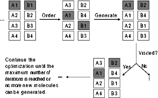
How the calculated gradients are used to obtain the next molecule within the LCAP framework is critical. The main idea is to use the LCAP gradients to choose the most promising fragment at each site. This scheme is best explained with a simple example for a framework with two fragment sites shown in Fig. 1. Each site has a library of four possible fragments. The current molecule is $A1B1$ as seen in Fig. 1. The LCAP gradients $\{\frac{\partial\beta_{zzz}}{\partial b_{A}^{\mathbf{R}}}^{\prime}\}$ are calculated for each fragment. For each site, all four functional groups are sorted in descending order according to their negative gradient values ($\{-\frac{\partial\beta_{zzz}}{\partial b_{A}^{\mathbf{R}}}^{\prime}\}$). In Fig. 1, the order after sorting becomes $A3>A1>A2>A4$ for site $A$, and $B2>B4>B1>B3$ for site $B$. Based on the ordering at each site, the next molecule is $A3B2$. If $A3B2$ has been visited before, one of the sites is chosen at random to undergo further mutation. As shown in Fig. 1, fragment $A3$ at site $A$ is replaced by fragment $A1$ (the next highest ranking fragment) and the new molecule $A1B2$ is generated. This procedure is repeated until a new molecule is obtained. However, because ab-initio calculations of the first hyperpolarizabilities are expensive, each design site will be mutated only once. As such, if a new molecule cannot be generated after several trial mutations or if the maximum number of iterations has been reached, the optimization stops. Using this procedure to generate a new molecule according to the normalized LCAP gradients, it is straightforward to implement the GDMC algorithm described in Section III to optimize NLO properties. The new GDMC-LCAP approach is tested in Section V.

In molecular design, the geometry changes of the target system have important effects on the target properties. In the current work, since we focus on optimizing the first hyperpolarizabilities of the extended $\pi$-electron structures with donors and acceptors, all of the candidate molecular structures are rigid. The substitutions at design sites do not disrupt the $\pi$-conjugation. Therefore, during the GDMC optimizations for three cases in V, the framework geometries were fixed.

V GDMC-LCAP optimization of the First hyperpolarizability

Extended $\pi$-electron structures with donors and acceptors are well known to have large first hyperpolarizabilities(Chen et al., 1994; Cheng et al., 1991a, b; Dehu et al., 1993; Di Bella et al., 1993; Garito et al., 1981; Kanis et al., 1994a, b; Lalama, 1981; Li et al., 1988; Marder et al., 1993; Meyers et al., 1994; Stiegman et al., 1991; Suslick et al., 1992; Misra et al., 2005), and their response properties are well understood in the context of both simple models and more involved quantum chemical calculations (Kanis et al., 1994b). Thus, our studies focus on donor-$\pi$-acceptor frameworks and one dominant tensor element, $\beta_{zzz}$, is computed and optimized. To explore the efficiency of the GDMC-LCAP approach, we optimized the absolute value of the first hyperpolarizability for three different $\pi$-electron conjugated scaffolds. The size of the cubic box in PWSCF(Baroni et al., 2002) was $22\times 22\times 22\ au^{3}$ in Case I, $30\times 30\times 30\ au^{3}$ in Case II, and $60\times 60\times 60\ au^{3}$ in Case III. The energy cutoff in the PWSCF calculation was 15 Ryd.(cut, ) The step size of the electric fields in Case I was $0.005au$ and was set to $0.0025au$ in Cases II and III (the smaller step size was used because of convergence issues during the SCF calculations). The functional used was LDA(Perdew and Zunger, 1981) and the maximum number of iterations was 30 except Case III, where it was 40. The empirical temperature parameter was also studied in three cases.

V.1 Case I

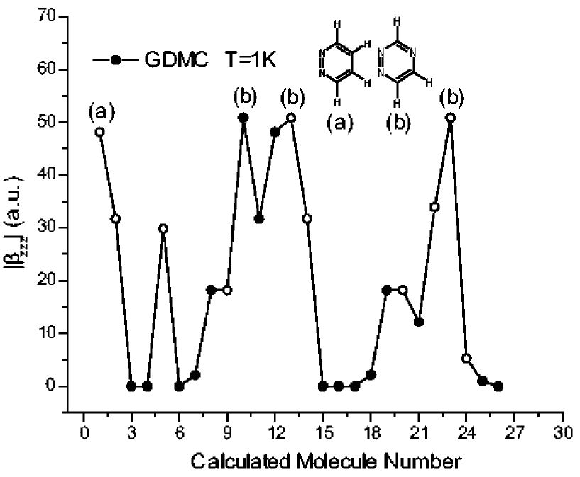
We first used a six-membered ring system to test the GDMC-LCAP optimization approach. The structural framework is shown in Fig.2. The geometry was taken from benzene ($r_{C-C}=1.390\AA$, $r_{C-H}=1.095\AA$) and was held fixed during the optimization. Either a $CH$ group or $N$ atom could be placed at each site, producing 64 possible structures (many are identical due to the rotational symmetry). The structures can also be enumerated to determine the largest $\beta_{zzz}$ value. From the enumeration, structure (b) in Fig. 3 was found to have the largest $\beta_{zzz}$ value.

The GDMC-LCAP optimization began with the initial molecule, structure (a) in Fig. 3, and the optimization profile is shown in Fig. 3. Five runs with different initial molecules were tested as well. They all yielded similar search profiles and produced structure (b). In Fig. 3, three degenerate molecules that had the same structure (b) (due to symmetry) were found. Since the initial structure (a) has a relatively large $\beta_{zzz}$ value, the optimization becomes trapped in this local optimum and the Monte Carlo stochastic moves were helpful in generating the next molecule and overcoming the barrier between local optima. From the $6th$ molecule in the profile, the LCAP gradients guided the molecular generation quite efficiently. In molecules $7-10$ generated from the LCAP gradient information, the absolute value of $\beta_{zzz}$ increased until the maximum value of $\beta_{zzz}$ was reached. The same behavior, led by local optimization based on the LCAP gradients, is also observed in the later steps shown in Fig. 3. The total number of molecular property calculations was only 26, and 14 jumps between molecules based on the LCAP gradients showed increased $\beta_{zzz}$ values. This indicates that the LCAP gradients indeed helped generating new molecules with increased property values.

V.2 Case II

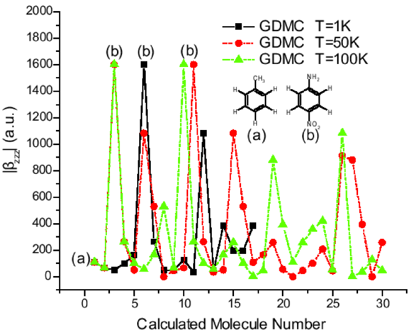
In Case II, a more complicated family of structures was explored. The structural framework is shown in Fig. 4. The six-member ring geometry is the same as in Case I. The geometries of the functional groups were generated using the Spartan Builder (spa, ). Either an $H$, $CH_{3}$, $NO_{2}$ or $NH_{2}$ fragment was placed at sites 1 and 2. Either a $CH$ or $N$ was placed at sites 3 through 6. Sites 1 and 2 are located on the z-axis. By enumerating all 256 possible structures, molecule (b) was found to have the largest $\beta_{zzz}$ value, shown in Fig. 5.

In Case II, at sites 1 and 2, the four functional groups have different numbers of electrons. When the continuous LCAP optimization is implemented, we observed that some “intermediate” molecules with a fractional number of electrons had large $\beta_{zzz}$ values. The fractional number of electrons is unphysical and makes the continuous surface rugged. However, in the GDMC-LCAP optimization, only the properties of real molecules are computed and the LCAP gradients direct the jumping from one molecule to another. Since this surface is more complicated, we tested the optimization using three different temperature parameters: $T=1K$, $50K$, and $100K$. All the optimizations began with the same initial molecule (a), shown in Fig. 5, and the optimization profiles are shown in Fig. 5.

All the GDMC-LCAP optimizations found the same molecule (b). When $T=1K$, only 17 molecules were computed and the best molecule was found in 2 jumps, indicated by the solid black line of Fig. 5 using the ordering of the LCAP gradients defined in Section IV. After the properties of 17 molecules were calculated, the optimization became trapped because of the low temperature. When the temperature was increased from $1K$ to $50K$, the GDMC protocol quickly jumped out of the local optimum around the initial molecule (a) in the beginning of the optimization, as shown by the dotted red line in Fig. 5. The largest $\beta_{zzz}$ molecule was obtained in the third property calculation. As the optimization continued at the higher temperature, GDMC generated new molecules that were more likely to be accepted based on their property values. The other degenerate molecule (b) was obtained in the eleventh property calculation. When the temperature was increased further to $100K$, the profile showed similar behavior. Basically, when $T$ varies from $1K$ to $100K$, GDMC has more flexibility to jump out of local optima and explore the discrete space more broadly.

V.3 Case III

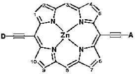
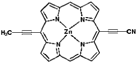
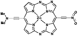
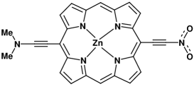
In Case III, a large porphyrin substituted donor-$\pi$-acceptor framework was used (see Fig. 6). The geometry was taken from molecule (c) in Fig. 7 that had been optimized at the $B3LYP/6-31+G*$ level using $Gaussian03$.(Frisch et al., ) The geometries of all donors and acceptors were generated using the Spartan Builder (spa, ). At site $A$, one of three acceptor groups ($NO_{2}$, $CN$ or $COH$) was placed. At site $D$, one of three donor groups ($N(CH_{3})_{2}$, $CH_{3}$ or $OCH_{3}$) was placed. Sites 1 through 10 have either a $CH$ or $N$ unit. This family of structures includes a total of 9,216 possible molecules. Performing ab initio first hyperpolarizability calculations on all of the possible structures is costly. Thus, we cannot enumerate all of the structures to find the one with the largest $\beta_{zzz}$ value.

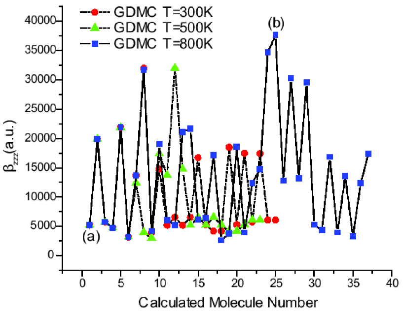
The initial molecule (a) consists of a normal porphyrin ring with a $CH_{3}$ at site $D$ and a $CN$ at site $A$ that were chosen randomly from four possible donors and four acceptors. Based on $\beta_{zzz}$ calculations for several initial molecules, the $\beta_{zzz}$ values vary from thousands to tens of thousands (in atomic units). Thus, we executed three GDMC optimizations at three different temperatures beginning with the initial molecule (a) shown in Fig. 7. The maximum number of iterations was 40. All of the optimization profiles are shown in Fig. 8. Two of the trajectories were trapped in local optima because the surface is rugged. The optimizations at $T=300K$ and $T=500K$ were stuck after less than 25 molecules were analyzed. At $T=800K$, GDMC jumped out of the local optimum and found one better molecule (b), shown in Fig. 7. However, we further tested five trial runs beginning from five different random initial molecules at $T=300K$. The most favorable molecule of all trial runs was molecule (b), shown in Fig. 7. This suggests that for much more rugged surface, the optimization is easily trapped when $T$ is not sufficiently high. Hence, for the low temperature such as $T=300K$ in this case, several independent optimizations with different random initial molecules allow more broad explorations of the molecular space. In addition, even for this rugged surface, the local gradient information from LCAP assists in jumping from one molecule to another with a higher $\beta_{zzz}$ value. For example, at $T=800K$, the $\beta_{zzz}$ value was increased from molecules 21 to 25 in the optimization profile.

The obtained molecule (b) shown in Fig. 7 contains a new type of porphyrin-like ring. The origin of its high $\beta_{zzz}$ becomes an interesting question. We speculate that, because nitrogen has more electrons than carbon, the four additional nitrogen atoms present in molecule (b) increase the number of $\pi$ electrons that are delocalized in the ring. In addition, the asymmetry of the broken ring facilitates polarization. Furthermore, molecule (b) has the strongest donor ($N(CH_{3})_{2}$) and acceptor ($NO_{2}$)(Kanis et al., 1994b) among the simple donor-acceptor structures. For these reasons, we predict that molecule (b) of Fig. 7 has a larger $\beta_{zzz}$ value than those with conventional porphyrin cores. Molecule (b) may represent a global optimum or a near optimal structure.

VI Conclusion

Although the original LCAP approach was demonstrated to optimize the first hyperpolarizability of simple systems efficiently(Wang et al., 2006), it suffers from the rugged surfaces when LCAP is applied for more complicated molecular libraries. During the property optimization, some “intermediate” or “alchemical” molecules were obtained with unphysically large first hyperpolarizabilities because of an unphysical fractional number of electrons. However, the LCAP gradients of the property with respect to the LCAP coefficients are useful in directing the search for candidate molecules. To utilize these LCAP gradients and to avoid analyzing “intermediate” molecules, we developed a gradient-directed Monte Carlo (GDMC) method that can be used in discrete optimization. After making the discrete space continuous, the property gradients with respect to the discrete variables can be calculated. The gradients are then used to generate a new set of discrete variables. The stochastic Monte Carlo moves assist in jumping out of local optima. Specifically, the LCAP gradients computed from one real molecule are normalized and utilized to generate a new structure. Therefore, the combined GDMC-LCAP approach was used to optimize the first hyperpolarizability for three different structural frameworks.

For Cases I and II, several runs of the GDMC-LCAP approach always found the most favorable structure that was validated by the exhaustive enumeration of all possible molecules. The jumps from one molecule to another based on the LCAP gradients have greater likelihood to increase the molecular first hyperpolarizability. The temperature used in GDMC-LCAP is an empirical parameter. When $T$ is sufficiently high, the optimization stops only if the maximum number of iterations is reached, for example, see Fig. 5 for Case II when $T=50K$ and $T=100K$. When $T$ is too low, the optimization is trapped after several trial mutations, for example, see Fig. 5 for Case II when $T=1K$ . To explore the molecular space more broadly when $T$ is low and ensure that the optimal property is found, several optimizations beginning from random initial molecules may be required. For example, in Case III, five trial runs beginning from five different random initial molecules at $T=300K$ were performed and structure (b) in Fig. 7 was obtained in all five runs. Furthermore, if GDMC is combined with heating, cooling, or annealing protocols, GDMC will be more robust and irrespective of the initial guess.

In Case III, the $\beta_{zzz}$ value of structure (b) in Fig. 7 obtained during the GDMC optimizations is increased almost $20\%$ compared to the initial seed molecule (a) in Fig. 7. In particular, the optimized structure has the strongest donor and acceptor groups at the $D$ and $A$ sites and a $\pi$-electron ring with four nitrogen atoms more than in a porphyrin. Thus, we predict that structure (b) in Fig. 7 is the optimal or nearly optimal structure.

To compare the GDMC method with other approaches such as the classical Monte Carlo (MC) method and a genetical algorithm (GA), we recently studied an HP model(Lau and Dill, 1989; Chan and Dill, 1991; Dill et al., 1995) for protein sequence design and protein folding.(Hu et al., 2008a) Those results indicate that the GDMC approach is much more efficient than the classical MC or GA optimization, because the property gradients with respect to the discrete variables, combined with the Monte Carlo moves, assist in jumping out of local optima and produce a greater likelihood of generating a new set of discrete variables with an enhanced property value.

When the geometry changes of frameworks are involved during the property optimization, the advantage of local searching directed by property gradients may not be clear. However, in a recent work, GDMC was employed to optimize protein sequence with concurrent protein structure optimization.(Hu et al., 2008b) It shows that GDMC is still more efficient than the classical MC.

In summary, the combined GDMC-LCAP approach provides an effective strategy for finding molecules with optimized molecular properties. The GDMC method can be used to explore other discrete spaces as well as the LCAP space.

Figure 1: Generation of a new molecule using LCAP gradients for GDMC optimization. Here, only two sites are considered. At each site, there are four possible fragments ($A1,A2,A3,A4$ for site $A$, and $B1,B2,B3,B4$ for site $B$). A gray box indicates that the fragment is present in the current molecule. Based on the LCAP gradients calculated for molecule $A1B1$, all of the fragments at each site are reordered and the next molecule $A3B2$ is generated. If $A3B2$ has been visited before, one site is randomly chosen to undergo mutation. In this example, site $A$ is chosen and fragment $A3$ is mutated to fragment $A1$ (the next highest ranking fragment) and $A1B2$ is generated. This procedure is repeated until the maximum number of iterations is reached or no more new molecules can be generated.

Figure 2: Framework for Case I. Either a $CH$ or $N$ can be placed at each site. 64 possible structures exist, without considering symmetry equivalent structures.

Figure 3: Optimization profile for Case I (T=1K). The x-axis indexes the calculated molecules during the optimization; the y-axis represents the absolute value of $\beta_{zzz}$, where empty circles denote negative molecular $\beta_{zzzz}$ values and solid circles denote positive values. The initial molecule is structure (a). Three degenerate molecules with structure (b) and the largest $\beta_{zzz}$ value were obtained. During the optimization, the LCAP gradients guided the generation of new molecules and resulted in a greater likelihood of generating a new molecule with a higher property value. The Monte Carlo random moves in the initial stage assisted in jumping out of the local optimum.

Figure 4: Framework for Case II. At sites 1 and 2, either an $H$, $CH_{3}$, $NO_{2}$ or $NH_{2}$ was placed. Either a $CH$ or $N$ was placed at sites 3 to 6. Sites 1 and 2 are located on the axis z. 256 possible structures exist, without considering symmetry equivalent structures.

Figure 5: Optimization profiles for Case II with three different temperature parameters. The largest $|\beta_{zzz}|$ molecule (b) was found in all optimizations. When $T$ is increased from $1K$ to $50K$ to $100K$, the other chemically identical molecule (b) was also found, suggesting that the optimization results do not depend critically on the temperature parameter.

Figure 6: Framework for Case III. At site $A$, one of three acceptor groups ($NO_{2}$, $CN$ or $COH$) was placed. At site $D$, one of three donor groups ($N(CH_{3})_{2}$, $CH_{3}$ or $OCH_{3}$) was placed. At sites 1 through 10, either a $CH$ or $N$ was placed. 9,216 possible molecules exist, without considering symmetry equivalent structures.

Figure 7: (a) Initial molecule in Case III. (b) Molecule with the largest $\beta_{zzz}$ value after four GDMC optimizations were carried out using three different temperature parameters. (c) Molecule with a normal porphyrin ring and the strongest donor and acceptor groups in Case III.

Figure 8: Three optimization profiles for Case III with three temperatures ranging from $300K$ to $800K$. $\beta_{zzz}$ values are always positive due to the donor-$\pi$-acceptor framework. The rugged surface trapped three optimizations when $T=300K$ and $500K$. At $T=800K$, GDMC jumped out of the local optimum and yielded molecule (b), shown in Fig. 7.

Figure 1:

Figure 2:

Figure 3:

Figure 4:

Figure 5:

Figure 6:

Figure 7:

Figure 8: