Photo-Solitonic Effect

Abstract

We show that dark solitons in 1D Bose liquids may be created by absorption of a single quanta of an external ac field, in a close analogy with the Einstein’s photoelectric effect. Similarly to the von Lenard’s experiment with photoexcited electrons, the external field’s photon energy $\hbar\omega$ should exceed a certain threshold. In our case the latter is given by the soliton energy $\varepsilon_{s}(\hbar q)$ with the momentum $\hbar q$, where $q$ is photon’s wavenumber. We find the probability of soliton creation to have a power-law dependence on the frequency detuning $\omega-\varepsilon_{s}/\hbar$. This dependence is a signature of the quantum nature of the absorption process and the orthogonality catastrophe phenomenon associated with it.

I Introduction

The existence of dark solitons (DS) is among the most spectacular manifestations of the role played by weak inter-particle interactions in 1D cold atomic gases SolitonObs . Such solitons are macroscopically large areas of partially, or even completely depleted gas, which propagate coherently without any dispersion. It is natural to interpret these objects as localized solutions of the semi-classical Gross–Pitaevskii equation SolitonTheory . Correspondingly, the means to create DS, employed so far, required a macroscopic classical perturbation applied to the atomic cloud. An example of the latter is the phase imprinting technique Imprinting , where a finite fraction of the 1D atomic cloud is subject to an external potential for a certain time. Once the potential is switched off and the gas is allowed to evolve, the DS is formed around the place with the maximal gradient of the potential.

Drawing an analogy with the electronic field-emission from a metal: a pulse of a strong external electric field may lead to creation of free electrons outside of the metal surface. It is well-known, however, from the time of von Lenard and Einstein Lenard ; Einstein that this is not the only way to excite electrons. Indeed, a weak ac field results in a photoelectric current, as long as the energy of its quanta exceeds the threshold given by the work function of the metal. The difference between the field-emission and the photoelectric effects is that the latter essentially utilizes the quantum nature of the electromagnetic radiation. Is there an analog of the photoelectric effect for excitation of DS? Namely can the DS be created by a weak ac radiation with the frequency exceeding a certain threshold?

In the framework of the Gross-Pitaevskii equation the answer on these questions is negative. Indeed, a weak external field may lead to excitation of the linear waves, if its wavenumber and frequency satisfy Bogoliubov dispersion relation, but not to creation of DS. However, treating the Bose liquid beyond the semiclassical Gross-Pitaevskii approximation reveals that creation of DS in response on an absorption of a single quanta with an above-the-threshold energy is actually possible. In analogy with the photoelectric effect we call this phenomenon the photo-solitonic effect. The threshold energy is given by the energy of DS $\varepsilon_{s}(p)$ with the momentum $p=\hbar q$, where $q$ is the photon wavenumber. Creation of DS requires an ac field with frequency $\hbar\omega>\varepsilon_{s}(p)$. Notice that no comparison of the external frequency $\omega$ and the DS energy $\varepsilon_{s}$ ever appears in the Gross-Pitaevskii treatment.

Consider 1D Bose liquid subject to an external ac potential with the wavenumber $q$ and frequency $\omega$. Such a radiation may be created using Bragg scattering technique Bragg1 ; Bragg2 . In these experiments the ac potential has been created by the interference pattern of two non-collinear optical beams with the differential frequency $\omega$ and the $x$-component of the differential wavevector $q$, [Bragg_foot, ]. At zero temperature, according to the fluctuation-dissipation theorem, the probability to absorb the radiation is given by the dynamic structure factor (DSF), defined as the density-density correlation function

$$S(q,\omega)=\int\!\!dxdt\,e^{i(qx-\omega t)}\left\langle\rho(x,t)\rho(0,0)\right\rangle\,,$$ (1)

where $\rho(x,t)$ is the density operator. Rewriting DSF in the Lehman representation in terms of exact many-body eigenstates of the system $|n\rangle$ with energies $\epsilon_{n}$, one finds

$$S(q,\omega)=\sum\limits_{n}\left|\langle n|\rho_{q}|0\rangle\right|^{2}\delta(\epsilon_{n}-\epsilon_{0}-\hbar\omega)\,,$$ (2)

where $\rho_{q}$ is the Fourier component of the density and $n=0$ corresponds to the ground state. Since the momentum is a good quantum number, only the many-body states with the total momentum $p=\hbar q$ contribute to the sum in the r.h.s. of Eq. (2).

For the model with the short-range repulsive interactions the many-body spectrum has been evaluated exactly using the Bethe ansatz (BA) method Lieb . Lieb has identified two characteristic modes in the excitation spectrum of the modelLieb , known as Lieb I and II modes with the dispersion relations $\varepsilon_{1,2}(p)$, Fig. 1. The two are given correspondingly by the particle and hole excitations in the set of the BA quasi-momenta. The hole-like mode $\varepsilon_{2}(p)$ is shown to be the lower bound of the many-body spectrum with a given momentum $p$. According to Eq. (2) absorption is only possible if $\hbar\omega>\varepsilon_{2}(\hbar q)$. Employing a numerical implementation of the algebraic BA Slavnov , Caux and Calabrese Caux06 have shown that DSF is indeed non-zero for all energies in excess of $\varepsilon_{2}(\hbar q)$ and is peaked at the particle-like mode $\hbar\omega=\varepsilon_{1}(\hbar q)$. In the limit of the weakly interacting gas the latter approaches the Bogoliubov dispersion relation Lieb ; Pitaevskii

$$\varepsilon_{1}(\hbar q)\to\hbar\omega_{B}(q)=v_{B}\hbar q\sqrt{1+(\hbar q/2mv_{B})^{2}}\,,$$ (3)

where $v_{B}$ is the Bogoliubov sound velocity and $m$ is the boson mass.

This observation offers a way to interpret absorption in a vicinity of the Lieb I mode, $\varepsilon_{1}(p)$, in terms of weakly interacting Bogoliubov quasiparticles. Consider, e.g., a photon with some wave vector $q$ and energy $\hbar\omega$ slightly below the value $\varepsilon_{1}(\hbar q)$, i.e., $\hbar\omega\lesssim\varepsilon_{1}(\hbar q)$, see point A in Fig. 1(a). The energy and momentum conservation laws allow for such photon to create two Bogoliubov quasiparticles, $\hbar\omega=\varepsilon_{1}(\hbar q-p)+\varepsilon_{1}(p)$. In the limit $\varepsilon_{1}(\hbar q)-\hbar\omega\ll mv_{B}^{2}$, one of the two particles has small momentum and may be viewed as a “soft” phonon. For smaller initial photon energies, the resulting two quasiparticles split the photon momentum more evenly, until the photon energy reaches the limiting value $\hbar\omega=2\varepsilon_{1}(\hbar q/2)$. If the photon energy is decreased below this threshold, a creation of more than two quasiparticles is needed to satisfy the conservation laws. Upon further lowering $\hbar\omega$, more quasiparticles are created in the process of photon absorption. Once the photon energy $\hbar\omega$ approaches the line $\varepsilon=v_{B}\hbar q$, Fig. 1, the energy and momentum of the absorbed photon is split between infinitely many soft phonons.

Below this line the described process of dividing the energy and momentum between the quasiparticles does not work any more. Nevertheless the many-body spectrum persists down to the lower value $\varepsilon_{2}(\hbar q)<v_{B}\hbar q$ and the algebraic BA calculations Caux06 show that there is a finite absorption probability in the energy window

$$\varepsilon_{2}(\hbar q)<\hbar\omega<v_{B}\hbar q\,.$$ (4)

What is the absorption mechanism in this window, where the conservation laws forbid excitation of any number of quasiparticles or phonons?

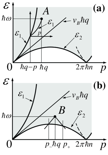
Figure 1: Momentum–energy plane for excitations. A photon is represented by a solid dot. (a) Absorption of a photon (dot marked by $A$) with energy and momentum slightly below the quasiparticle spectrum $\varepsilon_{1}(p)$, leads predominantly to creation of two quasiparticles with momenta $q-p$ and $p$ (the latter is determined by the shown geometrical construction). As $A$ approaches the line $\varepsilon=v_{B}p$, the number of excited quasiparticles increases. (b) Once photon energy-momentum (dot marked $B$) fall below the line $\varepsilon=v_{B}p$, its absorption involves creation of a soliton. Other excitations created in the course of absorption may be treated as phonons if $B$ is close to the boundary $\varepsilon_{2}(p)$. The shown “sound cone” with Bogoliubov velocity $v_{B}$ determines the range of possible momenta of a generated dark soliton, $p_{-}<p_{s}<p_{+}$.

The clue to answer this question appeared in the 1976 paper of Kulish, Manakov and Faddeev Kulish , who noticed that the hole-like Lieb II mode approaches dispersion relation of DS in the weakly interacting limit

$$\varepsilon_{2}(p)\to\varepsilon_{s}(p)\,.$$ (5)

It means that the many-body states with the energy in the vicinity of $\varepsilon_{2}$ must be viewed as quantized DS particles. Correspondingly the photon absorption in the energy window (4) necessarily involves excitation of DS along with Bogoliubov quasiparticles and/or phonons. Consider e.g. a photon with the energy immediately above the Lieb II mode, $\varepsilon_{2}<\hbar\omega\lesssim\varepsilon_{2}+mv_{B}^{2}$ (point B in Fig. 1 (b)). Drawing the “sound cone” with the slope $v_{B}$ down to the intersections with $\varepsilon_{2}(p)$, one finds the range of the possible momenta of DS

$$p_{-}<p_{s}<p_{+}\,,\quad\quad p_{\mp}=p_{\mp}(q,\omega)$$ (6)

which satisfy the conservation laws. Indeed, DS with the momentum $p_{-}$ accompanied by a phonon, propagating in the direction of the external momentum $\hbar q$, obviously satisfies the energy and momentum conservation. Similarly, DS with the momentum $p_{+}$ must be accompanied by the counter-propagating phonon. Any other soliton from the momentum window (6) requires excitation of a certain superposition of the forward and backward propagating phonons.

In this paper we evaluate probability $W_{q\omega}(p_{s})$ to excite DS with the momentum $p_{s}$ in the range (6) upon absorption of a photon with the wavenumber $q$ and frequency $\omega\geq\varepsilon_{2}(\hbar q)/\hbar$. We show that such a probability is heavily shifted towards the lower boundary of the interval $p_{s}=p_{-}(q,\omega)$, i.e. DS is preferentially excited along with the forward moving phonon. At larger photon energies, while still in the interval (4), DS is excited with highest probability along with the forward moving Bogoliubov quasiparticle. Its energy and momentum may be found geometrically by plotting the replica of the Bogoliubov dispersion curve which starts at some point along the Lieb II mode, $\varepsilon_{2}(p)$, and passes through the point $(\hbar q,\hbar\omega)$ representing external photon. We also show that the total probability to excite any DS scales as a power of the blue detuning from the energy threshold, $\int dp_{s}W_{q\omega}(p_{s})\propto(\hbar\omega-\varepsilon_{2})^{\mu_{2}}$. The exponent $\mu_{2}=\mu_{2}(q)$ is a function of photon wavenumber and the strength of interactions between the bosons. In the relevant limit of the weakly interacting gas, the exponent is large $\mu_{2}\gg 1$, signifying the relative smallness of the photo-solitonic effect. As we explain below, such a smallness is associated with the quantum orthogonality catastrophe phenomenon orthogonality .

The rest of this paper is organized as follows. In section II we reproduce a derivation of DS solution of the Gross-Pitaevskii equation to introduce notations and terminology. In section III we evaluate the probability to excite a specific DS upon absorption of a photon. Section IV is devoted to evaluation and discussion of DSF i.e. the total photon absorption rate, resulting in DS formation. Finally in section V we discuss ways to observe the effect experimentally along with the limitations of our theory.

II Dark Solitons

To establish notations let us briefly discuss the localized solutions of the non-linear Gross-Pitaevskii equationreview1999 . Quasiclassically, this equation is obeyed by the condensate wave function:

$$i\partial_{t}\Psi+\frac{1}{2m}\,\partial_{x}^{2}\Psi+c\left(n-|\Psi|^{2}\right)\Psi=0\,,$$ (7)

where $n=N/L$ is the average concentration and $L$ is the length of the system. Hereinafter we switch to the units with $\hbar=1$. The interaction strength $c$ determines Lieb the dimensionless parameter $\gamma=mc/n$ whose smallness $\gamma\ll 1$ is the criterion of the weak interaction.

Looking for a localized solution traveling with a certain velocity $v_{s}$, one substitutes

$$\Psi(x,t)=\Psi_{s}(x-v_{s}t)=\sqrt{n}\,\chi\,e^{i\vartheta}\,$$ (8)

in Eq. (7) and finds two equations for the phase $\vartheta(\xi)$ and the normalized amplitude $\chi(\xi)$, which are functions of $\xi=x-v_{s}t$. The first of these equations acquires the form of the continuity relation

$$\left[\chi^{2}\left(\vartheta\,^{\prime}-mv_{s}\right)\right]^{\prime}=0\,,$$ (9)

where primes denote derivatives with respect to $\xi$. Using the fact that far from the soliton $\chi(\pm\infty)=1$ and $\vartheta\,^{\prime}(\pm\infty)=0$, one finds $\vartheta\,^{\prime}=mv_{s}(1-1/\chi^{2})$. Employing this relation, the equation for the amplitude may be written in the form

$$\chi\,^{\prime\prime}=-\frac{\partial U(\chi)}{\partial\chi}\,,$$ (10)

where the effective potential $U(\chi)$, see Fig. 2, is given by

$$U(\chi)={m^{2}v_{s}^{2}\over 2}\left({1\over\chi^{2}}-{v_{B}^{2}\over v_{s}^{2}}\right)\left(1-\chi^{2}\right)^{2}\,,$$ (11)

with the Bogoliubov velocity $v_{B}=\sqrt{cn/m}$.

Figure 2: Effective potential $U(\chi)$ as given by Eq. (11) for (a) $v_{S}>v_{B}$; (b) $v_{S}<v_{B}$. The double-arrowed line designates the interval of variation of the normalized amplitude $\chi$ for physically allowed solutions of Eq. (10).

For $v_{s}>v_{B}$ the potential has the minimum at $\chi=1$ and the only physically acceptable solutions of Eq. (10) are small oscillations around this minimum. In a vicinity of $\chi=1$ the potential (11) may be approximated as $U\approx 2m^{2}(v_{s}^{2}-v_{B}^{2})(1-\chi)^{2}$ and therefore the small oscillation solutions have the form $\chi-1\sim\cos(q(x-v_{s}t))$ with $q=2m\sqrt{v_{s}^{2}-v_{B}^{2}}$. Rewriting the last expression as $v_{s}=v_{B}\sqrt{1+(q/2mv_{B})^{2}}$, one may recognize it as the phase velocity of the Bogoliubov mode. Correspondingly, the oscillation frequency $qv_{s}=\omega_{B}(q)$ coincides with Eq. (3). We thus conclude that the only solutions of GP equation which travel with a supersonic velocity are Bogoliubov quasiparticles.

The situation is more interesting for $v_{s}<v_{B}$. In this case the potential (11) exhibits a maximum at $\chi=1$, a minimum at a smaller amplitude and a turning point at $\chi=v_{s}/v_{B}<1$. The solution with the proper boundary conditions, $\chi(\pm\infty)=1$, is a trajectory which stays at the maximum and then exhibits a bounce down to the turning point and back to the maximum. This is the DS solution. To find it analytically, one may notice that Eq. (10) admits an integral of motion which for DS solution reads as

$${1\over 2}\,(\chi^{\prime})^{2}+U(\chi)=0\,.$$ (12)

Integrating this equation, one finds Tsuzuki1970 for the wave function (8)

$$\Psi_{s}=\sqrt{n}\left[\cos\frac{\theta_{s}}{2}-i\sin\frac{\theta_{s}}{2}\,\tanh\left(\frac{x-v_{s}t}{l_{s}}\right)\right],$$ (13)

where

$$\cos(\theta_{s}/2)=v_{s}/v_{B}$$ (14)

with $\theta_{s}$ being the change of phase of the wave function across the soliton. The soliton length $l_{s}$ is given by

$$l_{s}^{-1}=mv_{B}\sin(\theta_{s}/2)=m\sqrt{v_{B}^{2}-v_{s}^{2}}\,.$$ (15)

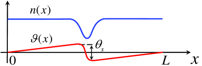
Figure 3: (color online) Density $n(x)$ and phase $\vartheta(x)$ profiles of a soliton in a system of length $L$. Note that the density perturbation is local, while the perturbation of phase is not.

The number of particles pushed away from the soliton core is

$$N_{s}=\int\!\!dx\left(n-|\Psi_{s}|^{2}\right)=\frac{2K}{\pi}\,\sin{\theta_{s}\over 2}\,,$$ (16)

where the “quantum parameter” $K=\pi n/(mv_{B})$ depends on the inter-particle interaction strength via the thermodynamic compressibility which defines the velocity $v_{B}$. Notice that the particle number may be very large, $N_{s}\gg 1$, in the limit of the weakly interacting gas ($K\gg 1$). The energy of the soliton is given by

$$\varepsilon_{s}=\int\!\!dx\left[{1\over 2m}|\partial_{x}\Psi_{s}|^{2}+{c\over 2}\left(n-|\Psi_{s}|\right)^{2}\right]={4nv_{B}\over 3}\sin^{3}{\theta_{s}\over 2}\,.$$ (17)

The calculation of DS momentum requires some care. The soliton core momentum, defined by the wave function (13) is

$$p_{sc}=\mbox{Im}\int\!\!dx\Psi_{s}^{*}\partial_{x}\Psi=-n\sin\theta_{s}\,.$$ (18)

However, one should take into account the periodic boundary conditions which ensure that DS phase shift $\theta_{s}$ is uniformly spread over the length of the entire system $L$, Fig. 3. Although this does not change the energy of the system in the thermodynamic limit (indeed the corresponding contribution to the energy scales as $n\theta_{s}^{2}/(mL)$), it produces a finite contribution $n\theta_{s}$ to the momentum. As a result the total (core plus the rest of the condensate) momentum of the DS state is

$$p_{s}=p_{sc}+n\theta_{s}=n\left(\theta_{s}-\sin\theta_{s}\right)\,.$$ (19)

Equations (17) and (19) give an implicit form of DS dispersion relation $\varepsilon_{s}(p_{s})$. The maximum of the soliton energy corresponds to $\theta_{s}=\pi$, where both the soliton velocity and core momentum vanish $v_{s}=p_{sc}=0$. The total momentum, however, is finite $p_{s}=\pi n$ and is uniformly spread across the entire condensate. This is the true DS, in a sense that the density vanishes in its center and the particle depletion reaches its maximal value $N_{s}=2K/\pi$. Away from the point $\theta_{s}=\pi$ soliton’s velocity is finite $v_{s}\neq 0$ as well as the density at any point. Because of the latter such solitons are sometimes called grey. Their velocity approaches sound velocity $v_{B}$ when the total momentum approaches zero or $2\pi n$, while the energy and $N_{s}$ both decrease. Clearly the concept of the classical soliton looses sense when the number of particles pushed away from the core is comparable to one, $N_{s}\lesssim 1$. This takes place when $\theta_{s}\lesssim 1/K\ll 1$, and therefore at $|p_{s}|\lesssim n/K^{3}$, and in intervals of the same width around the point $p=2\pi n$.

In the limit of the weak interactions $\gamma\ll 1$ (i.e. $K\gg 1$) the DS dispersion relation given by Eqs. (17), (19), approaches the Lieb II mode, plotted in Fig. 1. The convergence is not uniform and the two significantly deviate from each other in the narrow intervals of momenta near zero $|p_{s}|\lesssim nK^{-3/2}$ and similarly near $2\pi n$ [unpub, ]. Notice that at the boundaries of this interval the number of particles pushed away from the soliton core is still large $N_{s}\approx\sqrt{K}>1$. It is this condition, rather than the weaker one $N_{s}\gtrsim 1$, which determines the validity of the soliton approach. We shall return to this observation in section IV.

III Excitation of Dark Solitons

Consider a Bose gas subject to a weak space and time dependent external potential $V_{0}\cos(qx-\omega t)$. According to the Golden Rule (c.f. Eq. (2)), the system may absorb quanta of this field if its many-body spectrum possesses excited states with the momentum $q$ and energy $\omega$. It follows from the exactly solvable model Lieb that such states form a continuum whose energy is bound from below by the Lieb II mode $\varepsilon_{2}(q)$. As argued in the Introduction absorption of quanta with the energy in the range given by Eq. (4) is associated with creation of DS along with the phonons or quasiparticles.

To evaluate the probability of such a process it is convenient to think of it in terms of the space-time evolution of a state resulting from the photon absorption by the system initially in the ground state. To this end we notice that the photon absorption first creates a virtual state of the condensate with a local perturbation of the condensate wavefunction. Since the photon carries momentum $q$ and no extra particles, so does the initial local perturbation. Subsequently this perturbation evolves and eventually takes a form of a superposition of real excitations, i.e. conserving overall energy $\omega$ in addition to the momentum $q$. We expect that such a final state contains a soliton with the momentum $p_{s}\approx q$ and core energy $\varepsilon_{s}(p_{s})<\omega$. The small excess energy $\omega-\varepsilon_{s}>0$ is carried away by phonons, propagating with the sound velocity $v_{B}$.

The initial separation of the soliton core from a bunch of phonons takes a short time, which may be estimated as $\tau_{s}=l_{s}/v_{B}$. The soliton core is the density depletion, which carries momentum $-n\sin\theta_{s}$ (which is very different from $p_{s}\approx q$) and $-N_{s}$ particles. At times $t>\tau_{s}$ the core propagates without dispersion and behaves as a free particle with the energy $\varepsilon_{s}$. The remaining momentum $q+n\sin\theta_{s}\approx p_{s}+n\sin\theta_{s}=n\theta_{s}$, cf. Eq. (19), and $N_{s}$ particles, initially localized on a scale $\sim l_{s}$, must be carried away and spread over the entire system at $t\gg\tau_{s}$ by the phonons. As explained above, despite the fact that the phonons must carry away large number of particles $N_{s}$ and large momentum $n\theta_{s}$, their final energy is small, $\omega-\varepsilon_{s}\ll v_{B}n\theta_{s}$. Therefore this is the low-probability event, or the “under-barrier” process, which should be described as the imaginary time evolution Landau-Lifshitz ; LevitovShytov of the phonon system Matveenko .

To develop such a description we start from the imaginary time $\tau$ action for the interacting Bose field

$$S=\!\int\!d\tau dx\left[\bar{\Psi}\partial_{\tau}\Psi-{1\over 2m}|\partial_{x}\Psi|^{2}+cn|\Psi|^{2}-{c\over 2}\,|\Psi|^{4}\right].$$ (20)

It is convenient to parameterize the complex field as $\Psi=\sqrt{n+(\partial_{x}\varphi/\pi)}\,e^{i\vartheta}$, where $\varphi(x,\tau)$ and $\vartheta(x,\tau)$ are two real fields describing density and phase fluctuations correspondingly. Assuming small density fluctuations $\partial_{x}\varphi\ll\pi n$ and linearizing the resulting action, one finds

$$S=\!\int\!d\tau\left[{i\over\pi}\int\!dx\,\partial_{x}\varphi\,\partial_{\tau}\vartheta-H_{sw}\right]\,,$$ (21)

where the hydrodynamic Hamiltonian of the sound waves is given by Haldane

$$H_{sw}=\frac{\,v_{B}}{2\pi}\int\!dx\left[K^{-1}(\partial_{x}{\varphi})^{2}+K(\partial_{x}{\vartheta})^{2}\right]\,.$$ (22)

We have omitted terms $\sim(\partial_{x}^{2}\varphi)^{2}$ in the Hamiltonian, which is equivalent to restricting the spectrum of Bogoliubov quasiparticles to the phonon branch only. This approximation is sufficient for treating photon absorption close to the soliton threshold.

Taking the variations of the imaginary-time action over $\varphi$ and $\vartheta$, one finds the semiclassical equations of motion

$$\partial^{2}_{\tau x}\varphi+iv_{B}K\partial_{x}^{2}\vartheta = \pi N_{s}\left[\delta(x)\delta(\tau)-\delta(x-\bar{x})\delta(\tau-\bar{\tau})\right],$$

$$\partial^{2}_{\tau x}\vartheta+i{v_{B}\over K}\,\partial_{x}^{2}\varphi = \theta_{s}\left[\delta(x)\delta(\tau)-\delta(x-\bar{x})\delta(\tau-\bar{\tau})\right].$$

The right hand sides of these equations contain sources which describe the feedback of DS creation at the point $x=\tau=0$ and its subsequent destruction at the point $x=\bar{x}$, $\tau=\bar{\tau}$. As discussed above, such creation (destruction) of DS is associated with practically instantaneous and local injection (removal) of $N_{s}$ particles and momentum $n\theta_{s}$ into (out of) the phonon modes. The sources on the r.h.s. of the equations of motion do just that. The equations of motions are straightforwardly solved by the Fourier transformation. Substituting such a solution back into Eq. (21), one finds for the imaginary time action

$$S(\bar{x},\bar{\tau})=\mu_{+}\ln\left(1+\frac{\bar{x}-iv_{B}\bar{\tau}}{il_{s}}\right)+\mu_{-}\ln\left(1+\frac{\bar{x}+iv_{B}\bar{\tau}}{il_{s}}\right),$$ (23)

where we introduced notations

$$\mu_{\pm}=\frac{\left(K\theta_{s}\pm\pi N_{s}\right)^{2}}{4\pi^{2}K}=\frac{K}{\pi^{2}}\left(\frac{\theta_{s}}{2}\pm\,\sin\frac{\theta_{s}}{2}\right)^{2}$$ (24)

and employed Eq. (16) in the last equality in the r.h.s. of Eq. (24). Here $\theta_{s}$ is the parameter of a created DS, it is related to the DS momentum $p_{s}\approx q$ through Eq. (19). The soliton length $l_{s}$ appears in Eq. (23) as a short distance cutoff. Indeed, one should understand that the actual spatial (temporal) extent of the delta-functions on the r.h.s. of the equations of motions is the soliton size $l_{s}$ ($\tau_{s}=l_{s}/v_{B}$).

To find a probability of creating DS with the momentum $p_{s}$ upon absorbing a photon $(q,\omega)$, one needs to evaluate the Fourier transform of the square of the semiclassical matrix element given by $e^{-S}$. Specifically,

$$W_{q,\omega}(p_{s})=\mbox{Re}\!\int\!\!\frac{d\bar{x}\,d\bar{t}}{l_{s}}\,\,\,e^{-S(\bar{x},\bar{t})-i(q-p_{s})\bar{x}+i(\omega-\varepsilon_{s})\bar{t}},$$ (25)

where we took into account that the momentum $p_{s}$ and energy $\varepsilon_{s}(p_{s})$ are carried away by the soliton and therefore should not be absorbed by the phonons. The analytical continuation performed in Eq. (25) to the real frequencies $i\omega\rightarrow\omega$ is accompanied by the time integration contour (Wick) rotation $\bar{\tau}\rightarrow i\bar{t}$ to ensure convergence.

To evaluate the integral in Eq. (25), we take into account that for small energy excess $\omega-\varepsilon_{s}(q)\ll mv_{B}^{2}$ the range of the allowed soliton momenta $p_{s}$ is rather narrow, see Fig. 1 (b), and centered around the photon momentum $q$. One may therefore expand the soliton energy as $\varepsilon_{s}(p_{s})\approx\varepsilon_{s}(q)+(p_{s}-q)v_{s}$ and find for the boundaries of the possible soliton momenta, see Eq. (6) and Fig. 1 (b),

$$p_{\pm}(q,\omega)=q\pm\frac{\omega-\varepsilon_{s}(q)}{v_{B}\pm v_{s}(q)}\,;\quad\,\,\,\,p_{+}-p_{-}\ll p_{s}\,.$$ (26)

Adopting these notations and performing the straightforward integrations in Eq. (25), one finds

$$W_{q,\omega}(p_{s})\propto\frac{l_{s}}{v_{B}}\left[\frac{p_{+}-p_{s}}{l_{s}^{-1}}\right]^{\mu_{+}-1}\left[\frac{p_{s}-p_{-}}{l_{s}^{-1}}\right]^{\mu_{-}-1}\,.$$ (27)

Therefore the soliton creation rate is characterized by the power-law dependencies on the deviations of the soliton momentum from the upper and lower kinematic boundaries $p_{\pm}(q,\omega)$, Fig. 4 (a). The corresponding exponents $(\mu_{\pm}-1)$, see Fig. 4 (b), are functions of the soliton parameter $\theta_{s}=\theta_{s}(q)$ and the quantum parameter $K$ as given by Eq. (24). Since $\mu_{-}<\mu_{+}$, the probability to excite the soliton is heavily shifted towards the lower boundary $p_{-}$, Fig. 4(a). I.e. the soliton is preferentially accompanied by the forward moving phonons (in the direction of the photon momentum $q$).

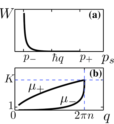
Figure 4: (a) Soliton creation rate as a function of the soliton momentum $p_{s}$. (b) Momentum dependence of the exponents $\mu_{\pm}$ for $K=10$.

IV Dynamic Structure Factor

Another quantity of interest is the total absorption rate of photons with a given $q$ and $\omega\gtrsim\varepsilon_{s}(q)$, which results in creation of a soliton with an unspecified momentum. This quantity is nothing but DSF $S(q,\omega)$ of the 1D Bose gas. Integrating $W_{q,\omega}(p_{s})$, Eq. (27), over the soliton momenta $p_{s}$, one finds for DSF in an immediate vicinity of the lower spectral boundary $\omega\gtrsim\varepsilon_{2}(q)$

$$S(q,\omega)=\int\limits_{p_{-}}^{p_{+}}\!dp_{s}\,W_{q,\omega}(p_{s})\propto{1\over v_{B}}\left(\frac{p_{+}-p_{-}}{l_{s}^{-1}}\right)^{\mu_{2}},$$ (28)

where the exponent is given by $\mu_{2}=\mu_{+}+\mu_{-}-1$. According to Eq. (24), the exponent is expressed through the parameters of the soliton $\theta_{s}$, which in turn is related to the soliton momentum through Eq. (19), where $p_{s}=q$. As a result

$$\mu_{2}(q)=\frac{2K}{\pi^{2}}\left[\left(\frac{\theta_{s}}{2}\right)^{2}+\left(\sin\frac{\theta_{s}}{2}\right)^{2}\right]-1\,.$$ (29)

For the true DS $\theta_{s}=\pi$ and therefore $\mu_{2}(\pi n)\approx 0.70K$. Notice that at $q\to 2\pi n$ Eq. (29) yields $\mu_{2}\approx 2K-1$, different from DSF exponent $K-1$ established in the framework of the Luttinger liquid theory Haldane . The latter is applicable above the dashed line in Fig. 1.

Employing Eq. (26), one may rewrite DSF (28) in the following form

$$S(q,\omega)\propto{1\over v_{B}}\left[\frac{\omega-\varepsilon_{s}(q)}{\Lambda(q)}\right]^{\mu_{2}(q)}\theta\left(\omega-\varepsilon_{s}(q)\right)\,,$$ (30)

where the cutoff energy is

$$\Lambda(q)=\frac{mv_{B}^{2}}{2}\,\sin^{3}\frac{\theta_{s}}{2}\approx\frac{\varepsilon_{s}(q)}{K}\,.$$ (31)

Being multiplied by the intensity of the radiation $V_{0}^{2}$, DSF gives a number of solitons excited per unit time and per unit length of the irradiated 1D gas.

The power law behavior of DSF near the lower spectral boundary $\varepsilon_{2}(q)\approx\varepsilon_{s}(q)$ was derived earlier by the present authors and M. Pustilnik in Ref. [bosons2007, ]. There a mapping between 1d Bose and Fermi systems was used to prove the presence of the power law non-analyticity and evaluate the exponent $\mu_{2}(q)$. However, the method adopted there allowed us to deduce the exponent only in the limit of strongly interacting bosons $\gamma\gg 1$ (since the latter is mapped onto weakly interacting fermions, treated in Ref. [Khodas2006, ]). Later a method to extract the edge exponent $\mu_{2}$ for an arbitrary interaction parameter from the BA solution was suggested in Refs. [Imambekov, ; Affleck-Pustilnik, ; Khodas-unp, ].

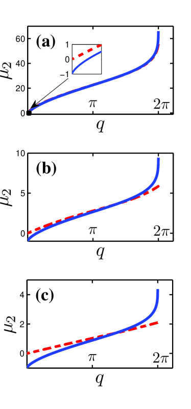
Figure 5: (color online) Edge exponent $\mu_{2}(q)$, cf. Eq. (30), as a function of momentum in units of $n$ for (a) $\gamma=0.05,\,K=33$; (b) $\gamma=0.4,\,K=5.2$; (c) $\gamma=1,\,K=2.7$. The full (blue) line is the semiclassical result (29); dashed (red) line is the Bethe ansatz solution of Ref. [Imambekov, ].

Fig. 5 shows comparison between the semiclassical result Eq. (29) and the numerical solution of BA equations Imambekov for the edge exponent $\mu_{2}$ as a function of the momentum (in units of $n$). The agreement between the two approaches becomes progressively better for weaker interactions (the only limit where the soliton picture holds, see Introduction). Such an agreement suggests that the interpretation of the photon absorption near the lower spectral edge as a formation of solitons is indeed consistent with a fully quantum many-body calculation. The latter Imambekov does not rely on existence of solitons at all. We consider it as a strong confirmation of the thesis that absorption of an ac quanta in the frequency window (4) results in the formation of DS.

Notice that even in the weakly interacting limit, the semiclassical prediction (29) deviates from the exact one at very small momenta, see the inset in Fig. 5(a). This is to be expected, since as was discussed in section II, the soliton picture looses its validity at sufficiently small momenta. Inspecting Eq. (29), one notices that the semiclassical exponent becomes negative at $\theta_{s}\lesssim\pi/\sqrt{K}$, contrary to the exact results, Fig. 5. Using Eq. (16), one finds that this corresponds to the number of missing particles in the soliton core $N_{s}\approx\sqrt{K}$. This observation collaborates with the discussion presented in the end of section II, which suggests that the semiclassical treatment looses validity for the very grey solitons with $N_{s}<\sqrt{K}$, i.e. $|p_{s}|<nK^{-3/2}$, cf. Eq. (19). We stress that the power-law behavior of DSF at the exact lower spectral boundary $\varepsilon_{2}(q)$ is valid for any momentum. However for $q<nK^{-3/2}$ the semiclassical approximation for the exponent $\mu_{2}(q)$ fails. Instead, the exact exponent bosons2007 ; Imambekov scales linearly with momentum $\mu_{2}(q)\sim K^{3/2}q/n$.

V Discussion

We have shown that the absorption of a photon with the energy above a certain threshold leads to formation of the DS. In the narrow energy window $\varepsilon_{s}<\omega<\varepsilon_{s}+\Lambda$ the total soliton formation rate per unit length of 1D Bose cloud is given by $S(q,\omega)V_{0}^{2}$, where DSF is given by Eq. (30) and $V_{0}\cos(\omega t-qt)$ is the external ac potential applied to 1D Bose gas. The momentum-resolved rate is given by Eq. (27), i.e., solitons with the momentum in the interval $p_{s}\pm dp_{s}/2$, where $p_{s}$ belongs to the window (6), are created with the rate $W_{q,\omega}(p_{s})V_{0}^{2}dp_{s}$.

An important question is what are the corresponding rates for a larger energy of the photon: $\varepsilon_{s}+\Lambda<\omega<v_{B}q$. According to the arguments given in the Introduction, absorption of such a photon should necessarily lead to DS formation. Yet our calculations are not directly applicable in this case. Indeed, we have used linearized dispersion relation for the quasiparticles (phonons) excited along with DS. For energies above $\varepsilon_{s}+\Lambda$ such an approximation is not valid. This is because Bogoliubov quasiparticles with momenta above $mv_{B}$ that take the excess energy can not be well approximated by phonons. The photon absorption is dominated by creation of a DS and single quasiparticle moving in the direction of the wavevector $q$ (i.e. moving forward). Thus the parameters of the typical DS may be found by plotting a replica of the Bogoliubov spectra which starts at some point along the absorption edge $\varepsilon=\varepsilon_{s}(q)$ and passes through $(q,\omega)$. The starting point prescribes DS momentum and energy. We expect that the power-law Eq. (30) saturates at an excess energy of order $\Lambda(q)$, i.e. at $\omega-\varepsilon_{2}\approx\Lambda$. As a result, DS formation rate per unit length may be estimated as $(V_{0}^{2}/\hbar^{2}v_{B})e^{-\alpha\mu_{2}(q)}$, with a numerical factor $\alpha\approx 1$.

Recalling that for a true DS $\mu_{2}=0.7K=1.1N_{s}$, one realizes that the photo-solitonic rate is exponentially suppressed with the increase of DS depleted particle number $N_{s}$. Physically the origin of this smallness is in the orthogonality phenomenon: the state of the system immediately after absorption of the photon is almost orthogonal to the state with the soliton causing a re-distribution of density and phase of the condensate in the one-dimensional system. The corresponding matrix element is exponentially small in the parameter $N_{s}$. This fact dictates a rather stringent limitations on the experimental observability of the photo-solitonic effect. Increasing interactions (i.e. decreasing $K$) makes the exponential factor in the photo-solitonic rate less severe, on the other hand it simultaneously decreases $N_{s}$, making it more difficult to observe the excited solitons. Assuming $V_{0}/(2\pi\hbar)=100\,\mathrm{Hz}$, Ref. [Bragg2, ] we estimate the soliton production rate for the relatively “light” solitons with $N_{s}=10$ as $1$ event per Bragg pulse of duration of $2$ seconds.

- (1) J. Denschlag, et al., Science 287, 97 (2000); S. Burger et al., Phys. Rev. Lett. 83, 5198 (1999); B.P. Anderson et al., Phys. Rev. Lett. 86, 2926 (2001).
- (2) R. Dum, et al., Phys. Rev. Lett. 80, 2972 (1998). Y. S. Kivshar, B. Luther-Davies, Phys. Rep. 298, 81 (1998). A. Muryshev et al., Phys. Rev. Lett. 89, 110401 (2002).
- (3) S. Burger et. al., Phys. Rev. Lett. 83, 5198 (1999). B. Wu, J. Liu, and Q. Niu, Phys. Rev. Lett. 88, 034101 (2002).
- (4) P. Lenard, Über die lichtelektrische Wirkung, Annalen der Physik, 8 (1902).
- (5) A. Einstein, On a Heuristic Viewpoint Concerning the Production and Transformation of Light, Annalen der Physik, 17 (1905).
- (6) J. Stenger et al., Phys. Rev. Lett. 82, 4569 (1999).
- (7) J. Steinhauer, R. Ozeri, N. Katz, and N. Davidson, Phys. Rev. Lett. 88, 120407 (2002); J. Steinhauer et. al., Phys. Rev. Lett. 90, 060404 (2003) and references therein.
- (8) In Bragg scattering tecnique strictly speaking, we talk about two-photon absorption.
- (9) E.H. Lieb and W. Liniger, Phys. Rev. 130, 1605 (1963); E.H. Lieb, Phys. Rev. 130, 1616 (1963).
- (10) N. A. Slavnov, Teor. Mat. Fiz. 79, 232 (1989); Teor. Mat. Fiz. 82, 389 (1990).
- (11) J.-S. Caux and P. Calabrese Phys. Rev. A 74, 031605 (2006).
- (12) E.M. Lifshitz and L.P. Pitaevskii, Statistical Physics, Part 2 (Pergamon Press, 1980).
- (13) P. P. Kulish, S. V. Manakov, L. D. Faddeev Theor. Mat. Fiz. 28, 38 1976.
- (14) P. W. Anderson, Phys. Rev. Lett. 18, 1049 (1967).
- (15) F. Dalfovo, S. Giorgini, L. P. Pitaevskii, and S. Stringari, Rev. Mod. Phys. 71, 463 (1999).
- (16) T. Tsuzuki, J. Low Temp. Phys. 4, 441 1970.
- (17) V. Gurarie, D. Gangardt, M. Khodas, A. Kamenev, and L.I. Glazman, unpublished.
- (18) L.D. Landau and E.M. Lifshitz, Quantum Mechanics, Non-Relativistic Theory (Pergamon Press, 1977).
- (19) L.S. Levitov and A.V. Shytov, Pis’ma Zh. Eksp. Teor. Fiz. 66, 200 (1997) [JETP Lett. 66, 214 (1997)] .
- (20) S. Brazovskii and S. I. Matveenko, Sov. Phys. JETP 96, 555 (2003) [Zh. Eksp. Teor. Fiz. 123, 625 (2003)]; S. Brazovskii and S. I. Matveenko, Phys. Rev. B 77, 155432 (2008).
- (21) V.N. Popov, Theor. Math. Phys. 11, 565 (1972); K.B. Efetov and I.A. Larkin, Sov. Phys. JETP 42, 390 (1975) [Zh. Eksp. Teor. Fiz. 69, 764 (1975)]; F.D.M. Haldane, Phys. Rev. Lett. 47, 1840 (1981).
- (22) M. Khodas, M. Pustilnik, A. Kamenev, and L.I. Glazman, Phys. Rev. Lett. 99, 110405 (2007).
- (23) M. Pustilnik, M. Khodas, A. Kamenev, and L. I. Glazman, Phys. Rev. Lett. 96, 196405 (2006).
- (24) A. Imambekov and L.I. Glazman, Phys. Rev. Lett. 100, 206805 (2008).
- (25) R. G. Pereira, S. R. White, and I. Affleck, Phys. Rev. Lett. 100, 027206 ( 2008); V. V. Cheianov and M. Pustilnik Phys. Rev. Lett. 100, 126403 (2008).
- (26) M. Khodas and A. Kamenev, unpublished.