Trace formula for dielectric cavities : I. General properties

Abstract

The construction of the trace formula for open dielectric cavities is examined in detail. Using the Krein formula it is shown that the sum over cavity resonances can be written as a sum over classical periodic orbits for the motion inside the cavity. The contribution of each periodic orbit is the product of the two factors. The first is the same as in the standard trace formula and the second is connected with the product of reflection coefficients for all points of reflection with the cavity boundary. Two asymptotic terms of the smooth resonance counting function related with the area and the perimeter of a convex cavity are derived. The coefficient of the perimeter term differs from the one for closed cavities due to unusual high-energy asymptotics of the $\mathbf{S}$-matrix for the scattering on the cavity. Corrections to the leading semi-classical formula are briefly discussed. Obtained formulas agree well with numerical calculations for circular dielectric cavities.

I Introduction

Only a limited number of quantum models permits exact analytical solutions. All others require either numerical or approximate approaches. One of the most useful approximation and widely used for non-integrable multi-dimensional quantum systems is the semiclassical one based on different types of trace formulas developed in the early 70’s balian_bloch ; gutzwiller_1 ; gutzwiller ; berry .

A general trace formula relates two different objects. Its left-hand side is the density of discrete energy levels, $E_{m}$, of a quantum system

$$d_{\mathrm{quantum}}(E)=\sum_{m}\delta(E-E_{m})\ .$$ (1)

The right-hand side of the trace formula is the sum of two contributions

$$d_{\mathrm{semi-classical}}(E)=\bar{d}(E)+d^{(osc)}(E)\ .$$ (2)

The first term, $\bar{d}(E)$, is the smooth part of level density given by a series of the Weyl terms (see e.g. balian_bloch and references therein). By definition, $\bar{d}(E)=\mathrm{d}\bar{N}(E)/\mathrm{d}E$ where $\bar{N}(E)$ is the mean number of levels with energies $E_{n}\leq E$ called also the smooth counting function. For two-dimensional billiards leading contributions to $\bar{N}(E)$ are the following

$$\bar{N}(E)=\frac{Ak^{2}}{4\pi}+r\frac{Lk}{4\pi}+\mathcal{O}(1)$$ (3)

where $k=\sqrt{E}$ is the momentum, $A$ is the area of the billiard cavity, and $L$ is its perimeter. $r$ in this formula is related with chosen boundary conditions. For example, $r=\pm 1$ for, respectively, the Neumann and the Dirichlet conditions.

The second term in (2), $d^{(osc)}(E)$, is the oscillating (or the fluctuating) part of the level density given in the leading order by the sum over classical periodic orbits

$$d^{(osc)}(E)=\sum_{\mathrm{periodic\ orbits}}d_{p}(E)+\mathrm{c.c.}$$ (4)

where $d_{p}(E)$ is the contribution of a given periodic orbit

$$d_{p}(E)=c_{p}\mathrm{e}^{\mathrm{i}S_{p}(E)/\hbar}\ .$$ (5)

Here $S_{p}(E)$ is the classical action along the periodic orbit (for billiards $S_{p}(E)=kl_{p}$ with $l_{p}$ being the length of the periodic orbit) and the prefactor $c_{p}$ can be computed from classical characteristics of the given periodic orbit (see below (24) and (25)). The trace formula is the statement that

$$d_{\mathrm{quantum}}(E)\stackrel{{\scriptstyle\hbar\to 0}}{{\longrightarrow}}d_{\mathrm{semi-classical}}(E)\ .$$ (6)

In an overwhelming majority of cases the trace formulas were applied to closed quantum systems with discrete energy levels. Though it is known (see e.g. gaspard ) that the trace formula and its modifications can also be applied for open quantum systems, only a small number of examples has been considered so far cvitanovic .

This is the first of a series of papers whose purpose is to demonstrate the usefulness of the application of trace formulas to open quantum systems, in particular, to dielectric cavities where a bounded domain is filled with a dielectric material with refractive index $n>1$ while the exterior is a media with refractive index $1$. The increasing interest to the investigation of such models to a large extend is related with their potential importance as resonators in micro-lasers nockel ; stone and the experimental possibilities of observing geometrical characteristics of the cavity from their lasing spectra melanie ; these_Melanie . The construction of trace formulas for dielectric cavities has been briefly discussed in these_Melanie . We also mention that for open chaotic resonators a variant of a trace formula has been developed in trace_openb .

Open systems, in general, have no discrete spectrum. So it is not immediately clear what should be the left-hand side (the spectral part) of the trace formula. In Section II we discuss the Krein formula krein_1 which is the main theoretical tool for open systems. This formula relates the excess density of states for an open cavity with the derivative over energy of the determinant of the $\mathbf{S}$-matrix for the scattering on the cavity. From the Krein formula it follows that the spectral part of the trace formula consists of the sum over all complex poles of the $\mathbf{S}$-matrix widely called resonances or quasi-stationary states.

The right-hand side of the trace formula should include a smooth part and a sum over periodic orbits (cf. (2)). The general formalism like the multiple scattering approach, used by Balian and Bloch in their construction of the trace formula for closed cavities balian_bloch , is not yet fully developed for dielectric cavities. The main difference of dielectric cavities from closed ones is that for the later one knows boundary conditions on the cavity boundary but for the former boundary conditions are fixed only at infinity. Due to this fact the resulting integral equation (13) includes the integration over the cavity volume and not over its boundary as for the closed case which complicates the general construction. In Section III the form of leading periodic orbit contributions is fixed from physical considerations.

To get more insight to this problem, in Section IV a simple example of integrable circular dielectric cavity is considered in detail. Despite the calculations are straightforward, they permit us to calculate in Section V the smooth part of the counting resonance function and in Section VI the periodic orbit contributions. In Section VII we consider main corrections to the asymptotic results and, in particular, demonstrate how the Goos-Hänchen shift g_h manifests in the trace formula. All obtained formulas agree well with numerical calculations.

Though these results were obtained, strictly speaking, only for circular dielectric cavities, all main steps leading to them are quite general and we conjecture that they remain valid for dielectric cavities of arbitrary shape. The detailed comparison of the derived trace formulas with numerical calculations for cavities of different shapes is postponed for a future publication part_II .

II Krein formula

Throughout this paper we focus on a planar two-dimensional domain $\mathcal{D}$. The wave equations widely used for such dielectric cavities are the following (see e.g. jackson )

$$(\Delta+n^{2}E)\Psi(\vec{x}\,) = 0\mbox{ when }\vec{x}\in\mathcal{D}\ ,$$

$$(\Delta+E)\Psi(\vec{x}\,) = 0\mbox{ when }\vec{x}\notin\mathcal{D}\ .$$ (7)

In electromagnetism we rather consider the wavenumber $k=\sqrt{E}$, which is related to the frequency $\omega$ of the wave through $k=\omega/c$, c being the speed of light in the vacuum. For simplicity we shall suppose that the wave function, $\Psi(\vec{x}\,)$, and its normal derivative are continuous along the boundary of $\mathcal{D}$. In electrodynamics these boundary conditions correspond to transverse magnetic (TM) modes inside an infinite dielectric cylinder with cross section $\mathcal{D}$ jackson . Transverse electric (TE) modes may be treated similarly and will be considered elsewhere.

We stress that Eqs. (7) describe correctly electromagnetic fields only for an infinite dielectric cylinder. For a real 3-dimensional cavity with a small height, $h$, they have to be modified. The authors are not aware of the full 3-dimensional treatment of such problems. The usual approach consists to consider the refractive index, $n$, in these equations not as a constant but as an effective refraction index, $n=n_{eff}(kh)$, for the motion inside a 2 dimensional dielectric slab (see e.g. nous and references therein) but errors of a such approximation are not known at present.

The possibility of using such cavities as resonators is related with the phenomenon of the total internal reflection. It is known (see e.g. jackson ) that if the TM plane wave inside the cavity is reflected from a straight boundary, the (Fresnel) coefficient of reflection has the following form

$$R(\theta)=\left\{\begin{array}[]{cc}\dfrac{n\cos\theta-\sqrt{1-n^{2}\sin^{2}\theta}}{n\cos\theta+\sqrt{1-n^{2}\sin^{2}\theta}},&\textrm{ when }|\theta|<\theta_{c}\\ \dfrac{n\cos\theta-\mathrm{i}\sqrt{n^{2}\sin^{2}\theta-1}}{n\cos\theta+\mathrm{i}\sqrt{n^{2}\sin^{2}\theta-1}},&\textrm{ when }|\theta|>\theta_{c}\end{array}\right.\ .$$ (8)

Here $\theta$ is the angle between the direction of the incoming wave and the normal to the boundary and the critical angle

$$\theta_{c}=\arcsin 1/n\ .$$ (9)

When $|\theta|>\theta_{c}$ $|R(\theta)|=1$ and the wave is completely reflected from the boundary which may lead to formation of long-lived states. We mention that this expression becomes less efficient for curved boundary close to the critical angle (see e.g. felsen_marcuvitz ).

Eq. (7) admits only continuous spectrum and its properly renormalized eigenvalue density, $d(E)$, has to be a smooth function of energy, contrary to closed systems where the level density is a sum of delta’s peaks (cf. (1)). It is convenient to rewrite (7) as the Schrödinger equation with a potential

$$(\Delta+E)\Psi(\vec{x}\,)=-\lambda V(\vec{x}\,)\Psi(\vec{x}\,)$$ (10)

where the coupling constant

$$\lambda=E(n^{2}-1)$$ (11)

and the potential $V(\vec{x}\,)$ is non-zero only inside the cavity

$$V(\vec{x}\,)=\left\{\begin{array}[]{cc}1&\mbox{ when }\vec{x}\in\mathcal{D}\\ 0&\mbox{ when }\vec{x}\notin\mathcal{D}\end{array}\ .\right.$$ (12)

Except of unusual dependence of the coupling constant on the energy this equation describes the motion in a finite-range potential so standard methods (see e.g. s_matrix ) can be applied to analyze it. In particular, its solution corresponding to the continuous spectrum is defined by the following integral equation (see also rawlings )

$$\Psi(\vec{x}\,)=\mathrm{e}^{\mathrm{i}\vec{k}\vec{x}}-\lambda\int_{\mathcal{D}}G_{0}(k|\vec{x}-\vec{y}\,|)\Psi(\vec{y}\,)\mathrm{d}\vec{y}$$ (13)

where $\vec{k}$ is the momentum vector of the incoming wave with coordinates $k(\cos\,\theta,\sin\,\theta)$, $G_{0}(k|\vec{x}-\vec{y}\,|)$ is the free Green function of the left-hand side of (10)

$$G_{0}(z)=\frac{1}{4\mathrm{i}}H^{(1)}_{0}(z),$$ (14)

and $H^{(1)}_{0}(z)$ is the Hankel function of the first order.

This equation may serve as a starting point of the multiple scattering method similar to the one discussed in balian_bloch . The important difference between these two cases is that the integration in (13) is performed over the whole cavity volume which complicates the iteration procedure. Nevertheless, Eq. (13) has the standard form of the Fredholm equation and its solutions are well defined similar to the usual case when coupling constant $\lambda$ is independent of energy. In particular, from (13) it follows that the $\mathbf{S}$-matrix for the scattering on the cavity has the form

$$\mathbf{S}(\theta,\theta^{\prime})=\delta(\theta-\theta^{\prime})+\frac{\mathrm{i}\lambda}{4\pi}f(\theta,\theta^{\prime})$$ (15)

where $\theta$ and $\theta^{\prime}$ are the angles determining the directions of, respectively, incoming and outcoming waves and

$$f(\theta,\theta^{\prime})=\int_{\mathcal{D}}\mathrm{e}^{-\mathrm{i}\vec{k^{\prime}}\vec{y}}\Psi(\vec{y}\,)\mathrm{d}\vec{y}\ .$$ (16)

Here $\vec{k^{\prime}}$ is the momentum of the outgoing wave with coordinates $k(\cos\theta^{\prime},\sin\theta^{\prime})$.

The importance of the $\mathbf{S}$-matrix lies in the fact that the excess density of states for open systems can conveniently be written through it by using the Krein formula (see krein_1 and lifshitz ; birman_1 ). This formula relates the density of states of two operators: the first with a short-range potential, $d(E)$, and the second without it, $d_{0}(E)$. In physical terms it reads

$$d(E)-d_{0}(E)=\frac{1}{2\pi\mathrm{i}}\frac{\partial}{\partial E}\ln\ \mathrm{det}\ \mathbf{S}(E)$$ (17)

where $\mathrm{det}\ \mathbf{S(E)}$ is the determinant of the $\mathbf{S}$-matrix for the scattering on the potential. For clarity in Appendix A a physical ’derivation’ of this formula is given in the simplest case of one-dimensional systems.

It is also known (see e.g. s_matrix , sect. 12, and zworski_3 ; poisson ) that function det $\mathbf{S}(E)$ for the scattering on a finite-range potential is a meromorphic function in the complex $k\equiv\sqrt{E}$ plane with (in even-dimensional spaces) a cut along the negative $k$-axis

$$\mathrm{det}\ \mathbf{S}(E)=\mathrm{e}^{\mathrm{i}f(k)}\prod_{m}\frac{k-k_{m}^{*}}{k-k_{m}}$$ (18)

where $k_{m}$ with Im $k_{m}<0$ denote the positions of the poles of the $\mathbf{S}$-matrix on the second sheet of energy surface and the product is taken over all such poles. (Terms which ensure the convergence of this infinite product are not written explicitly). Here $f(k)$ is a certain function without singularities in the cut complex plane related with the asymptotics of the $\mathbf{S}$-matrix when $E\to\infty$. Due to the symmetry $k\to-k$ of (7), if $k_{m}$ is a pole, $-k_{m}^{*}$ will also be a pole which is implicitly assumed in (18).

Therefore, the left-hand side of (17) can be written as the sum over all poles of the $\mathbf{S}$-matrix

$$d(E)-d_{0}(E) = g(E)-\frac{1}{2\pi k}\sum_{m}\mathrm{Im\ }\frac{1}{k-k_{m}}$$ (19)

$$= g(E)-\frac{1}{\pi}\sum_{m}\mathrm{Im\ }\frac{1}{E-E_{m}}$$

where $E_{m}=k_{m}^{2}$ and $g(E)=f^{\prime}(k)/2\pi$. In mathematical literature such formulas are known as Poisson formulas (see poisson and references therein).

From (19) it is clear that poles of the $\mathbf{S}$-matrix, especially those close to the real axis, play an important role in $d(E)$ as they produce peaks in the otherwise smooth background.

The positions of these poles, called also resonances or quasi-stationary states, are in principle determined from Eq. (7) by an analytic continuation of the $\mathbf{S}$-matrix from the real axis to the complex plane, in a similar way as in main_wiersig . Another way is to impose the outgoing radiation conditions (see e.g. s_matrix )

$$\Psi(\vec{x}\,)\propto\mathrm{e}^{{\mathrm{i}}k|\vec{x}|}\;\mbox{ when }|\vec{x}|\to\infty\ .$$ (20)

These conditions select a well defined set of complex eigenvalues $E_{m}$ whose imaginary parts correspond to the resonance lifetime $\tau_{m}$, $\mathrm{Im\ }E_{m}=-1/2\tau_{m}$.

These arguments demonstrate that the spectral part of the trace formula (the analog of (1)) may be written as the sum over all poles (= resonances) of the $\mathbf{S}$-matrix

$$d_{\mathrm{quantum}}(E)=-\frac{1}{\pi}\sum_{m}\frac{\mathrm{Im\ }E_{m}}{(E-\mathrm{Re\ }E_{m})^{2}+(\mathrm{Im\ }E_{m})^{2}}$$

$$=-\frac{1}{2\pi k}\sum_{m}\frac{\mathrm{Im\ }k_{m}}{(k-\mathrm{Re\ }k_{m})^{2}+(\mathrm{Im\ }k_{m})^{2}}\ .$$ (21)

When Im $E_{m}\to 0$ one recovers the usual $\delta$-function contribution.

III General properties of trace formulas for dielectric cavities

To find the right-hand side of trace formula one has to express it through the Green function. In this section we will only consider the real continuous spectrum of Eq. (7) and eigenfunctions associated with it. We will not deal with functions associated with the resonances defined by boundary condition (20). A minor difference with the usual case of closed systems consists in the fact that the eigenfunctions are orthogonal not with respect to the standard scalar product $\int\Psi_{E_{1}}^{*}(\vec{r}\,)\Psi_{E_{2}}(\vec{r}\,)\mathrm{d}\vec{r}$ but to a modified one

$$\int n^{2}(\vec{r}\,)\Psi_{E^{\prime}}^{*}(\vec{r}\,)\Psi_{E^{\prime\prime}}(\vec{r}\,)\mathrm{d}\vec{r}=\delta(E^{\prime}-E^{\prime\prime})$$ (22)

where the integration is performed over the whole space. Here $n(\vec{r}\,)=n$ for points inside the cavity and $n(\vec{r}\,)=1$ outside it. This relation can easily be checked from the main equation (7).

This modification leads to the following formal relation between the density of states and the trace of the Green function (cf. e.g. balian_bloch )

$$d(E)=-\frac{1}{\pi}\int n^{2}(\vec{r}\,)\mathrm{Im\ }G_{E}(\vec{r},\vec{r}\,)\mathrm{d}\vec{r}\$$ (23)

where the integration is extended to the whole space.

Exactly as for closed systems (see e.g. balian_bloch ; gutzwiller_1 ; gutzwiller ), the dominant contribution to the fluctuating part of the density of states comes from classical periodic orbits. When saddle point is considered, it is clear that the only information that a trajectory may have about a boundary is contained in the reflection coefficient from this boundary. Therefore, the principal difference with the closed systems is that the contribution of a given periodic orbit has to be multiplied by the product of reflection coefficients (8) for all bounces with the cavity boundary (which we called the total reflection coefficient) and the later can be less than unity.

These simple arguments demonstrate that for dielectric cavities the dominant contribution of a periodic orbit to the density of states when $k\to\infty$ has the following form

• For an isolated primitive periodic orbit $p$ repeated $r$ times

  $$d_{p}(E)=\frac{nl_{p}}{\pi k\ |\det(M_{p}^{r}-1)|^{1/2}}R_{p}^{r}\mathrm{e}^{\mathrm{i}[rnkl_{p}-r\mu_{p}\pi/2]}$$ (24)

  where $l_{p},M_{p},\mu_{p}$, $R_{p}$ are, respectively, the length, the monodromy matrix, the Maslov index, and the total reflexion coefficient for the chosen primitive periodic orbit.

• For a primitive periodic orbit family

  $$d_{p}(E)=\frac{n^{3/2}\mathcal{A}_{p}}{\pi\ \sqrt{2\pi rkl_{p}}}\langle R_{p}^{r}\rangle\mathrm{e}^{\mathrm{i}[rkl_{p}-r\mu_{p}\pi/2+\pi/4]}$$ (25)

  where $\mathcal{A}_{p}$ is the area covered by periodic orbit family, $\langle R_{p}^{r}\rangle$ is the mean over family value of the total reflection coefficient, and all other notations are as above.

The dependence on $n$ of the prefactors in these formulas is related with the fact that inside the cavity the momentum equals $nk$.

Now we have all ingredients of the trace formula for dielectric cavities except the smooth (Weyl) terms (3). It is clear that its value depends on how many $\mathbf{S}$-matrix resonances are included in the right-hand side of the trace formula (21). Energy eigenvalues of closed systems are real and they all have to be included. For open systems resonance energies are complex and a natural approach is to take into account only resonances whose imaginary part is restricted, e.g. $-\mathrm{Im\ }k_{m}<\gamma$. Other resonances (if any) have to be considered as a smooth background. This separation of poles is, to a large extent, arbitrary which manifests in the fact that the smooth part of the resonance density will be now a function of $\gamma$ whose calculation is a difficult problem.

For 2-dimensional open chaotic billiard problems with holes there exist strong arguments zworski_1 ; zworski_2 that the leading term of the Weyl law is non-trivial

$$\bar{N}(E)\sim C(\gamma)k^{\nu}$$ (26)

where $\nu<2$ is related with the fractal dimension of the trapped set of classical orbits.

For open dielectric cavities arguments leading to (26) can not be directly applied and it appears nonnenmacher that in this case standard estimates (3) with different constants are valid. In general, there exist two types of resonances whose behavior is different when the system is somehow ”closed”. The first (sometimes called Feshbach or internal resonances) are resonances which tends to eigenvalues of the corresponding closed system and the second ones (called shape or outer resonances) are those whose imaginary part remains non-zero when a system is closed. The both types of resonances exist for dielectric cavities (see e.g. nous ). In all cases with convex shaped cavities considered by us these two groups of resonances are well separated and there exists a clearly defined value of $\gamma_{\mathrm{max}}$ such that all first type resonances have $-\mathrm{Im\ }k_{m}<\gamma_{\mathrm{max}}$. It does not contradict main_wiersig where a Fractal Weyl law was argued to be a good description of a part of the resonance spectrum with small imaginary part. In the next section we shall argue that when all these resonances are taken into account the smooth counting function $\bar{N}(E)$ defined as the mean number of resonances with $\mathrm{Re}\,E_{n}<E\equiv k^{2}$ and $-\mathrm{Im\ }k_{m}<\gamma_{\mathrm{max}}$ is similar to (3) but with following modifications

$$\bar{N}(E)=\frac{An^{2}k^{2}}{4\pi}+\tilde{r}(n)\frac{Lk}{4\pi}+\mathcal{O}(1)$$ (27)

where $A$ and $L$ are, as above, the area and the perimeter of the cavity but $\tilde{r}(n)$ is

$$\tilde{r}(n)=1+\frac{n^{2}}{\pi}\int_{-\infty}^{\infty}\frac{\mathrm{d}t}{t^{2}+n^{2}}R(t)-\frac{1}{\pi}\int_{-\infty}^{\infty}\frac{\mathrm{d}t}{t^{2}+1}R(t)$$ (28)

and

$$R(t)=\dfrac{\sqrt{t^{2}+n^{2}}-\sqrt{t^{2}+1}}{\sqrt{t^{2}+n^{2}}+\sqrt{t^{2}+1}}\ .$$ (29)

The function $r(n)$ can be expressed through elliptic integrals. It is monotonic function of $n$ starting from $1$ for $n=1$ and tending to $n(4/\pi-1)$ for large $n$.

Finally, the trace formula for dielectric cavities has the following form

$$- \frac{1}{\pi}\sum_{-\mathrm{Im\ }k_{m}<\gamma_{\mathrm{max}}}\frac{\mathrm{Im\ }k_{m}}{(k-\mathrm{Re\ }k_{m})^{2}+(\mathrm{Im\ }k_{m})^{2}}$$ (30)

$$= 2k\{\bar{d}(E)+\sum_{p}[d_{p}(E)+d_{p}^{*}(E)]\}\ .$$

Here $d_{p}(E)$ for isolated periodic orbits is given by (24) and for periodic orbits from a family it is defined in (25). The factor $2k$ in the right-hand side is introduced as we found it more convenient to work with the density of states as a function of momentum.

To see the effect of periodic orbit it is usual to multiply the both sides of the trace formula (30) by a test function, e.g. by $\mathrm{e}^{-\mathrm{i}knl}$, and integrate over $k$ in a certain window $k_{1}<k<k_{2}$ which includes many resonances. The dominant contribution in the left-hand side of this formula is the sum over resonances whose momentum is restricted $k_{1}<\mathrm{Re\ }k<k_{2}$ and $0<-\mathrm{Im\ }k_{m}<\gamma_{\mathrm{max}}$

$$\sum_{m}\mathrm{e}^{-\mathrm{i}k_{m}nl}\simeq\sum_{p}I_{p}(l)$$ (31)

where the summation is done over periodic orbits, $p$, and it is implicitly assumed that term with $p=0$ corresponds to the smooth part of the trace formula. Here $I_{p}$ denotes the integral the individual periodic orbit contribution given by (24) or (25)

$$I_{p}(l)=\int_{k_{1}}^{k_{2}}\mathrm{e}^{-\mathrm{i}knl}d_{p}(E)2k\mathrm{d}k$$ (32)

which is strongly peaked at the periodic orbits length. Eq. (31) is called the length density.

Periodic orbits are not the only contributions to the trace formula. For polygonal cavities important contributions are given by diffractive orbits which go through singularities of the boundary (see e.g. pavloff and references therein). Usually their individual contribution is smaller than those of periodic orbits. The careful calculation of such corrections requires the knowledge of the diffraction coefficient on dielectric singularities which is not available analytically. We shall also not discuss here creeping orbits (see e.g. creeping and references therein) corresponding to the external motion along cavity boundary as they are responsible only for shape resonances and their contributions are small.

IV Circular cavity

The circular dielectric cavity is one example of a two-dimensional cavity with an explicit analytical solution and it is instructive to illustrate the above general formulas in this simple case.

The Green function $G(\vec{r},\vec{r}^{\ \prime},E)$ for this problem has been written e.g. in nous . From that formulas it follows that inside the circular cavity with radius $R$ the Green function $G(\vec{r},\vec{r},E)$ with $r<R$ has the form

$$G(\vec{r},\vec{r}\,) = -\frac{1}{2\pi x}\sum_{m\in\mathbb{Z}}\frac{J_{m}^{2}(nkr)}{s_{m}(x)J_{m}^{2}(x)}$$ (33)

$$+ \frac{1}{4\mathrm{i}}\sum_{m\in\mathbb{Z}}\frac{J_{m}(nkr)}{J_{m}(nx)}g_{in}(r)$$

where

$$g_{in}(r)=J_{m}(nx)H^{(1)}_{m}(nkr)-J_{m}(nkr)H^{(1)}_{m}(nx)\ ,$$ (34)

and outside it (when $r>R$) it is

$$G(\vec{r},\vec{r}\,) = -\frac{1}{2\pi x}\sum_{m\in\mathbb{Z}}\frac{H^{(1)\ 2}_{m}(kr)}{s_{m}(x)H^{(1)\ 2}_{m}(x)}$$

$$+ \frac{1}{4\mathrm{i}}\sum_{m\in\mathbb{Z}}\frac{H^{(1)}_{m}(kr)}{H^{(1)}_{m}(x)}g_{out}(r)$$

with

$$g_{out}(r)=H^{(1)}_{m}(x)J_{m}(kr)-J_{m}(x)H^{(1)}_{m}(kr)\ .$$ (36)

Here $x\equiv kR$, $J_{m}(z)$ (resp. $H^{(1)}_{m}(z)$) stands for the Bessel function (resp. the Hankel function of the first kind), and

$$s_{m}(x)=n\frac{J_{m}^{\prime}}{J_{m}}(nx)-\frac{H^{(1)\prime}_{m}}{H_{m}^{(1)}}(x)\ .$$ (37)

Quantities $s_{m}(x)$ are of special importance as the positions of resonances, $x_{m}\equiv k_{m}R$, are determined by their complex zeros (see e.g. nous )

$$s_{m}(x_{m})=0\ .$$ (38)

Using the formula bateman

$$\int^{x}A_{\nu}(t)B_{\nu}(t)t\mathrm{d}t = \frac{x^{2}}{2}A_{\nu}^{\prime}(x)B_{\nu}^{\prime}(x)$$ (39)

$$+ \frac{x^{2}-\nu^{2}}{2}A_{\nu}(x)B_{\nu}(x)$$

valid for any two Bessel functions $A_{\nu}(z)$ and $B_{\nu}(z)$ of the same arguments and performing straightforward calculations one gets

$$d(E)-d_{0}(E)=\frac{R^{2}(n^{2}-1)}{2\pi x}\sum_{m=-\infty}^{\infty}\mathrm{Im\ }\frac{1}{s_{m}(x)}$$ (40)

where $d(E)$ is formally

$$d(E)=2\pi\Big{[}n^{2}\int_{0}^{R}+\int_{R}^{A}\Big{]}\mathrm{Im\ }G(\vec{r},\vec{r}\,)r\mathrm{d}r$$ (41)

and

$$d_{0}(E)=2\pi\int_{0}^{A}\mathrm{Im\ }G_{0}(\vec{r},\vec{r}\,)r\mathrm{d}r$$ (42)

with the free Green function

$$G_{0}(\vec{r},\vec{r}^{\ \prime})=\frac{1}{4\mathrm{i}}H^{(1)}_{0}(k|\vec{r}-\vec{r}^{\ \prime}|)\ .$$ (43)

In the above formulas it is assumed that the cut-off $A\gg R$ and the limit $A\to\infty$ is taken after the subtraction $d(E)-d_{0}(E)$.

The calculation of the $\mathbf{S}$-matrix for the circular dielectric cavity is also well known debye and one finds

$$\mathbf{S}_{m}(E)=-\frac{H^{(2)}_{m}(x)s_{m}(x)^{*}}{H^{(1)}_{m}(x)s_{m}(x)}$$ (44)

with $s_{m}(x)$ are defined in (37). It is straightforward to check that (40) can be written in the form

$$d(E)-d_{0}(E)=\frac{1}{2\pi\mathrm{i}}\frac{\partial\ }{\partial E}\ln\det\ \mathbf{S}(E)$$ (45)

which is the Krein formula (17) for the dielectric disk.

In Figs. 1a) and b) we present numerically computed from (38) positions of complex momenta of quasi-bound states for dielectric circular cavities with $n=1.5$ and $n=2$.

a)

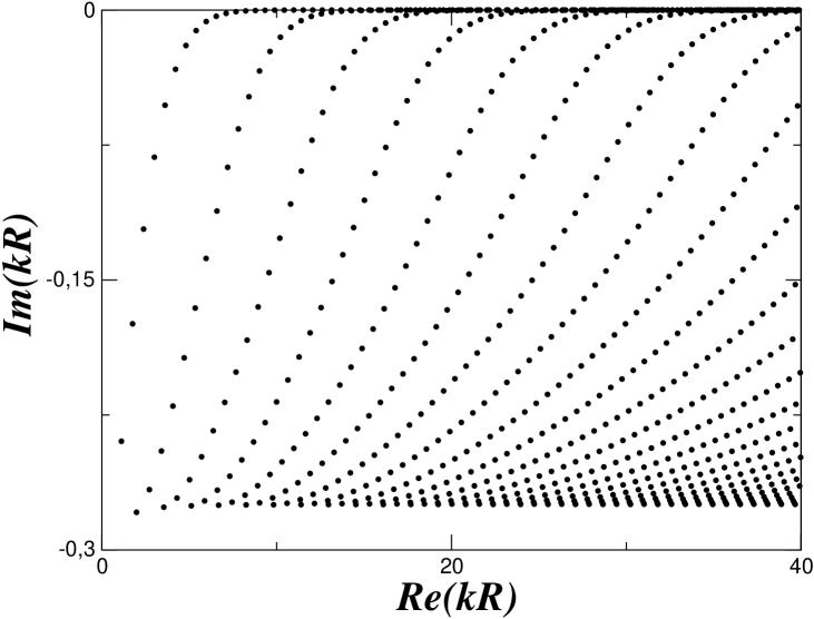
b)

Figure 1: a) Resonance spectrum for the dielectric circular cavity with $n=1.5$ and Re $kR<100$. b) The same but for $n=2$ and Re $kR<40$.

Clearly, resonances in this case are organized in families corresponding to conserved quantum numbers of radial and angular momenta (see e.g. nous ). Let notice that for large Re $kR$ imaginary parts of all resonances obey the inequality

$$-\mathrm{Im}\ kR\leq\gamma_{\mathrm{max}}(n)$$ (46)

where

$$\gamma_{\mathrm{max}}(n)=\frac{1}{2n}\ln\frac{n+1}{n-1}\ .$$ (47)

$\gamma_{\mathrm{max}}(1.5)\approx.5365$ and $\gamma_{\mathrm{max}}(2)\approx.2765$ in a very good agreement with Fig. 1a) and b). This bound corresponds to the imaginary part of zeros of $s_{m}(x)$ with $m=0$ and large $x$ and can be proved from semiclassical approximation to (37). Physically, it is natural that all the states have a leakage smaller than a particle moving along the diameter of the circle.

As was mentioned above, the resonances in Figs. 1a) and b) are not the only existing quasi-bound states of the dielectric disk. It is known (see e.g. nous ) that functions $s_{m}(x)$ have another series of zeros corresponding to the shape (or outer) resonances, $\tilde{x}_{m,p}$, also depending on 2 quantum numbers $m$ and $p$.

Figure 2: Outer (shape) resonances for the dielectric circular cavity with $n=1.5$ Dashed line indicates the lowest bound (47) for imaginary parts of resonances in Fig. 1a)

At Fig. 2 some of these resonances are plotted. Notice the difference in the vertical scale of this figure in comparison with Figs. 1a) and b). All resonances at Fig. 1a) are situated above the dashed line in Fig. 2. In nous it was shown that positions of these outer resonances are described asymptotically by the equation

$$\dfrac{H_{m}^{(1)\prime}}{H_{m}^{(1)}}(\tilde{x}_{m,p})=\mathrm{i}\sqrt{n^{2}-\frac{m^{2}}{\tilde{x}_{m,p}^{2}}}\ .$$ (48)

Its solutions with the smallest modulus of the imaginary part have $\tilde{x}_{m,p}\approx m$ and are close to complex zeros of the Hankel function in the denominator of this equation. In nous it is shown that in this case

$$\tilde{x}_{m,p}=z_{m,p}-\frac{\mathrm{i}}{\sqrt{n^{2}-m^{2}/z_{m,p}^{2}}}+\mathcal{O}(\mathrm{Im}\,z_{m,p}/\mathrm{Re}\,z_{m,p})$$ (49)

where $z_{m,p}$ is a complex zero of $H_{m}^{(1)}(z)$ function. It is known bateman that at the principal Riemann sheet of $H_{m}^{(1)}(z)$ cut along the negative part of the real axis such zeros have negative imaginary parts, lie symmetrically with respect to the imaginary axis, and for integer $m$ there is $[m/2]$ zeros with positive real part. These Hankel zeros with the lowest imaginary part can asymptotically be computed by the expansion (see e.g. nous )

$$z_{m,p}=m+\eta_{p}\left(\frac{m}{2}\right)^{1/3}\mathrm{e}^{-2\pi\mathrm{i}/3}+\mathcal{O}(\eta_{p}^{2}/m^{1/3})$$ (50)

and $\eta_{p}$ is the modulus of the $p^{\mathrm{th}}$ zero of the Airy function ($p=1,2,\ldots$). With a good precision these Airy zeros are described by the semiclassical formula

$$\frac{2}{3}\eta_{p}^{3/2}\approx\pi(p-\frac{1}{4})\$$ (51)

which works well even for small $p$. In general, shape resonances of dielectric circular cavity are situated at $\mathcal{O}(1)$ distances from shape resonances of circular cavity with Dirichlet boundary conditions.

From the above arguments it follows that the additional resonances have quite large imaginary parts and are located below the curve

$$-\mathrm{Im}\,x<\mathrm{const}\ |\mathrm{Re}\,x|^{1/3}$$ (52)

so they are well separated from the main resonances obeying (46). This bound has been proved trapping_orbits , zworski_sjostrand for the scattering on any smooth $(C^{\infty})$ convex cavity provided no trapping orbits exist. If the cavity boundary is not smooth only the weaker bound is known martinez

$$-\mathrm{Im}\,x<\mathrm{const}\ \log|\mathrm{Re}\,x|\ .$$ (53)

V Weyl’s law

The circular cavity is useful to find the Weyl law (28) for the smooth part of the counting function. As usual (see e.g. uzy ), it can be extracted by considering pure imaginary values of momentum $k=\mathrm{i}s$ and calculating the asymptotics of the Bessel functions from the known formulas (see e.g. bateman ). In this manner one gets

$$\mathrm{i}s_{m}(\mathrm{i}s)=\sqrt{\frac{m^{2}}{s^{2}}+n^{2}}+\sqrt{\frac{m^{2}}{s^{2}}+1}$$

$$- \frac{n^{2}s}{2(m^{2}+n^{2}s^{2})}+\frac{s}{2(m^{2}+s^{2})}+\mathcal{O}(s^{-2})\ .$$

Changing the summation over $m$ in (40) into the integration from $-\infty$ to $\infty$ one obtains that two main terms of the smooth part of the right hand side of (40) have the following form

$$\langle\frac{\partial\ }{\partial E}\ln\det\ \mathbf{S}(E)\rangle=\frac{A}{4\pi}(n^{2}-1)+[r(n)-1]\frac{L}{8\pi k}+\mathcal{O}(k^{-3})\$$ (55)

where $r(n)$ is defined in (28).

But this formula gives the asymptotic behavior of the determinant of the full $\mathbf{S}$-matrix which is not necessarily related directly with cavity resonances. According to (44) the $\mathbf{S}$-matrix for the dielectric circular cavity is the product of 2 factors

$$\mathbf{S}_{m}(E)=\mathbf{S}_{m}^{(0)}(E)\mathbf{S}_{m}^{(1)}(E)$$ (56)

where

$$\mathbf{S}_{m}^{(0)}(E)=-\frac{H^{(2)}_{m}(x)}{H^{(1)}_{m}(x)}$$ (57)

and

$$\mathbf{S}_{m}^{(1)}(E)=\frac{s_{m}^{*}(x)}{s_{m}(x)}\ .$$ (58)

It is easy to check that the $\mathbf{S}^{(0)}$-matrix is the $\mathbf{S}$-matrix for the scattering on a circular disk with the Dirichlet boundary conditions whose asymptotic behavior is known (see e.g. uzy and references therein)

$$\langle\frac{\partial\ }{\partial E}\ln\det\ \mathbf{S}^{(0)}(E)\rangle=-\frac{A}{4\pi}-\frac{L}{8\pi k}+\mathcal{O}(k^{-3})\ .$$ (59)

The matrix element $\mathbf{S}_{m}^{(1)}(E)$ is the ratio of 2 functions: $s_{m}(x)$ defined in (37) and its complex conjugate. It is convenient to rewrite it as the ratio of two other functions

$$\mathbf{S}_{m}^{(1)}(E)=\frac{F_{m}^{*}(x)}{F_{m}(x)}\$$ (60)

where

$$F_{m}(x)=\left[nJ_{m}^{\prime}(nx)-J_{m}(nx)\frac{H^{(1)\,\prime}_{m}(x)}{H^{(1)}_{m}(x)}\right]x^{m-1}\ .$$ (61)

The factor $x^{m-1}$ is introduced to insure that $F_{m}(x)$ tends to a constant independent on $x$ when $m\to\infty$.

The function $F_{m}(x)$ has 2 groups of zeros (cf. (38)). The first includes all usual resonances which obeys the inequality (46) and the second consists of additional resonances (shape resonances) with large imaginary part (52). But it has also a series of poles coming from zeros of the Hankel function $H_{m}^{(1)}(x)$. According to (49) the position of shape resonances in two leading orders differs from the corresponding zero of the Hankel function only by a finite shift. From the bound (52) it follows also that for a finite $\gamma>0$ there is only a finite number of additional resonances whose imaginary part obeys the inequality $\mathrm{Im}k<-\gamma$.

These two arguments demonstrate that with a big precision additional resonances and poles of the Hankel functions corresponding to shape resonances of the external Dirichlet problem cancel each other. It means that function $F_{m}(x)$ can be considered as having effectively only resonances with small imaginary parts. Consequently, the mean value of $(\ln\det\ \mathbf{S}^{(1)})^{\prime}$ gives the average value of the counting function of resonances. From (56) it follows that the later equals to the difference between (55) and (59)

$$\langle\frac{\partial\ }{\partial E}\ln\det\ \mathbf{S}^{(1)}(E)\rangle$$

$$= \langle\frac{\partial\ }{\partial E}\ln\det\ \mathbf{S}(E)\rangle-\langle\frac{\partial\ }{\partial E}\ln\det\ \mathbf{S}^{(0)}(E)\rangle$$

which finally leads to the asymptotics (27). A careful separation of the internal and external resonances in higher order corrections remains an open problem.

The fact that in order to find the smooth part of the resonance counting function for a dielectric cavity in the leading order one has to divide the determinant of the $\mathbf{S}$-matrix for the scattering on this cavity by the determinant of the $\mathbf{S}$-matrix for the scattering on the same cavity but with the Dirichlet boundary condition may physically be argumented as follows. In the semiclassical limit a small part of a smooth boundary can be considered as a straight segment. Resonances inside the cavity can be determined from the knowledge of the reflection coefficient from this part of the boundary as it is done in the Appendix A. It is easy to see that the $\mathbf{S}$-matrix corresponding to the reflection from outside the cavity differs just by a sign from the reflection coefficient inside the cavity. But the $\mathbf{S}$-matrix equals $-1$ is exactly the $\mathbf{S}$-matrix for the scattering on the cavity with the Dirichlet boundary conditions which explains the above statement.

For a symmetric cavity it is convenient to split resonances according to their symmetry representations. Often it equivalent to consider a smaller cavity where certain boundaries are true dielectric boundaries but on others parts of the boundary one may have in the simplest cases either Dirichlet or Neumann boundary conditions. Now the total boundary contribution to the mean counting function can be written as follows

$$\frac{1}{4\pi}\left(n(L_{N}-L_{D})+r(n)L_{0}\right)k\ .$$ (63)

Here $L_{N}$ and $L_{D}$ are the lengths of the boundary parts with respectively Neumann and Dirichlet boundary conditions and $L_{0}$ is the length of the true dielectric interface.

The knowledge of the spectrum for dielectric disk (cf. Fig. 1) permits us to check the derived formula for the mean counting function. First we count how many resonances exist with real part less than a fixed value, Re $k_{m}<k$. These resonances have to be taken into account with their multiplicities. For the circular cavity states with $m\neq 0$ are double degenerated and states with $m=0$ are simple. Then the resulting curves are fit by a polynomial of second degree with the highest term equals $n^{2}Ak^{2}/4\pi$. As for $R=1$, $A=\pi$ and $L=2\pi$, one gets the following fits:

• For $n=1.5$:

  $$\bar{N}(k)=\frac{2.25}{4}k^{2}+\mathbf{.5139}k+.1518\ .$$ (64)

• For $n=2$:

  $$\bar{N}(k)=k^{2}+\mathbf{.5446}k+.034\ .$$ (65)

The quality of the fits can be seen from Fig. 3 where the differences between numerically calculated counting functions and the above fits are plotted.

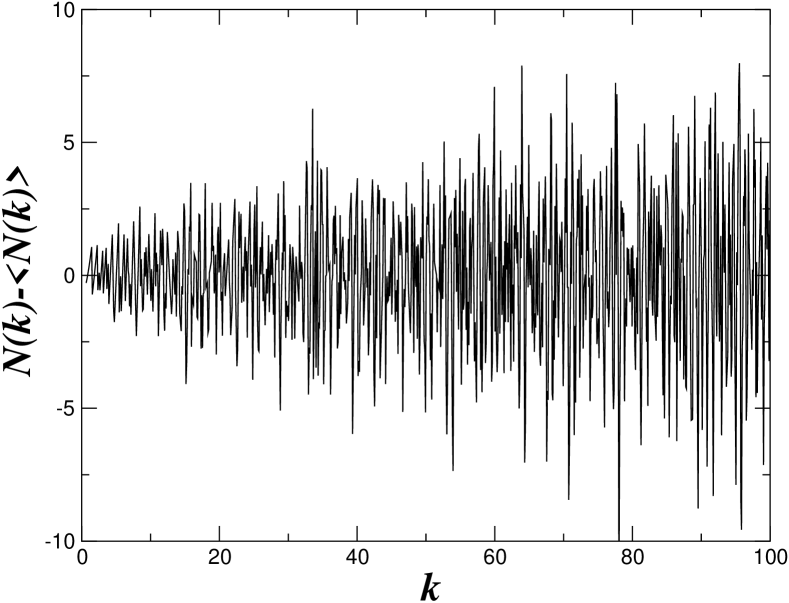
a)

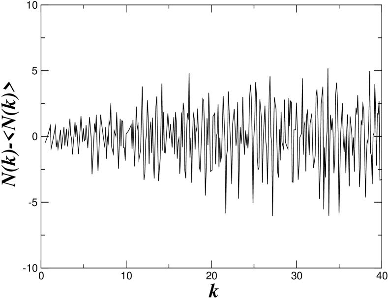
b)

Figure 3: Difference between the exact counting functions of resonances of circular cavity with unit radius and their quadratic fits (64) and (65): (a) for $n=1.5$, (b) for $n=2$.

The theoretical prediction for the coefficient of the linear in $k$ term is $\tilde{r}(n)/2$ where $\tilde{r}(n)$ is defined in (28). Numerically one finds that these coefficients should be equal to $\mathbf{.5125}$ for $n=1.5$ and to $\mathbf{.5420}$ for $n=2$ in a good agreement with the above numerical fits.

VI Periodic orbit contribution

To get oscillating contributions to the trace formula for a circular cavity we start from the expression (40). Expressing the Bessel function in (37) through the Hankel functions of the first and the second kinds $J_{m}(x)=(H_{m}^{(1)}(x)+H_{m}^{(2)}(x))/2$ and performing straightforward transformations of $s_{m}(x)$ in (37) one gets a formal series for the density of states

$$d(E)-d_{0}(E)=\frac{R^{2}}{2\pi x}\sum_{m=-\infty}^{\infty}\mathrm{Im}\,\left[\frac{n^{2}-1}{B_{m}(x)}\right.$$ (66)

$$+\left.\frac{4\mathrm{i}}{\pi x}\sum_{r=1}^{\infty}P_{m}(x)[R_{m}^{(\mathrm{e})}(x)]^{r}E_{m}^{r}(x)\right].$$

Using the Poisson summation formula, the sum over $m$ can be substituted by the integration over $m$ and the summation over a conjugate integer $M$

$$d(E)-d_{0}(E)=\frac{R^{2}}{4\pi\mathrm{i}x}\sum_{M=-\infty}^{\infty}\int_{-\infty}^{\infty}\mathrm{d}m\,\mathrm{e}^{2\pi\mathrm{i}Mm}$$ (67)

$$\times\left[\frac{n^{2}-1}{B_{m}(x)}+\frac{4\mathrm{i}}{\pi x}\sum_{r=1}^{\infty}P_{m}(x)[R_{m}^{(\mathrm{e})}(x)]^{r}E_{m}^{r}(x)\right]+\mathrm{c.c.}$$

Here the following notations have been introduced

$$E_{m}(x)=\frac{H_{m}^{(1)}(x)}{H_{m}^{(2)}(x)}\ ,$$ (68)

$$R_{m}^{(\mathrm{e})}(x)=-\frac{A_{m}(x)}{B_{m}(x)}\ ,$$ (69)

$$A_{m}(x)=n\frac{H_{m}^{(1)\prime}}{H_{m}^{(1)}}(nx)-\frac{H_{m}^{(1)\prime}}{H_{m}^{(1)}}(x)\ ,$$ (70)

$$B_{m}(x)=n\frac{H_{m}^{(2)\prime}}{H_{m}^{(2)}}(nx)-\frac{H_{m}^{(1)\prime}}{H_{m}^{(1)}}(x)\ ,$$ (71)

and

$$P_{m}(x)=(n^{2}-1)\left(H_{m}^{(1)}(nx)H_{m}^{(2)}(nx)A_{m}(x)B_{m}(x)\right)^{-1}.$$ (72)

No approximation has been done in Eq. (67) and it can serve as a starting point for derivations of dominant terms and corrections to them. In the semiclassical limit $x\to\infty$ it can be simplified by using standard asymptotics of the Hankel function bateman

$$H_{m}^{(1)}(x)\simeq\frac{\sqrt{2/\pi}}{(x^{2}-m^{2})^{1/4}}\mathrm{e}^{\mathrm{i}\phi_{m}(x)}$$

$$\times\left[1-\frac{b_{1}(x)}{\sqrt{x^{2}-m^{2}}}+\mathcal{O}(x^{-2})\right]$$ (73)

where

$$\phi_{m}(x)=\sqrt{n^{2}x^{2}-m^{2}}-m\arccos\left(\frac{m}{nx}\right)-\frac{\pi}{4}$$ (74)

and

$$b_{1}(x)=\frac{1}{8}-\frac{5}{24}(1-x^{2}/m^{2})^{-1}\ .$$ (75)

In this manner one concludes that, when $x\to\infty$ and $|m|<nx$, $E_{m}(x)\to\mathrm{e}^{2\mathrm{i}\phi_{m}(x)}$, $P_{m}(x)\to\sqrt{n^{2}-m^{2}/x^{2}}$, and

$$R_{m}^{(\mathrm{e})}(x)\to R_{m}(x)=\frac{\sqrt{n^{2}-m^{2}/x^{2}}-\sqrt{1-m^{2}/x^{2}}}{\sqrt{n^{2}-m^{2}/x^{2}}+\sqrt{1-m^{2}/x^{2}}}\ .$$ (76)

From these equations it follows that the dominant periodic orbit contribution is

$$d^{(osc)}(E)=\frac{R^{2}}{4\pi x}\sum_{M=-\infty}^{\infty}\sum_{r=1}^{\infty}$$ (77)

$$\times\int_{-\infty}^{\infty}\mathrm{d}m\sqrt{n^{2}-\frac{m^{2}}{x^{2}}}R_{m}^{r}(x)\mathrm{e}^{\mathrm{i}S_{M,r}(m)}+\mathrm{c.c.}$$

where the action (the phase of the exponent)

$$S_{M,r}(m)=2\pi Mm+2r\phi_{m}(x)\ .$$ (78)

The last step, as usual, consists in the computation of the integral over $m$ by the stationary phase method. The saddle point value of $m=m_{sp}$ is determined from the equation

$$\frac{\partial}{\partial m}S_{M,r}(m)=0$$ (79)

whose solution

$$m_{sp}=nx\cos\theta_{M,r}$$ (80)

with

$$\theta_{M,r}=\pi\frac{M}{r}$$ (81)

corresponds geometrically to the periodic orbit of the circular cavity in the shape of regular polygon with $r$ vertices going around the center $M<r$ times. If $M$ and $r$ are co-prime integers the periodic orbit is primitive. Otherwise, it corresponds to a primitive periodic orbit repeated $d$ times where $d$ is the largest common factor of $M$ and $r$.

The action (78) can be expanded into a series of deviation from from the saddle point value $m=m_{sp}+\delta m$. One gets

$$S_{M,r}(m_{sp}+\delta m)=nkl_{p}-\frac{\pi}{2}r+\frac{g_{2}}{2}\delta m^{2}+\mathcal{O}(\delta m^{3})$$ (82)

where $l_{p}$ is the periodic orbit length

$$l_{p}=2rR\sin\theta_{M,r}$$ (83)

and $g_{2}$ is the second derivative of the action computed at the saddle point

$$g_{2}=\frac{2r}{nx\sin\theta_{M,r}}\ .$$ (84)

Computing the integral over $m$ by the saddle point approximation one gets the expected result (25)

$$d^{(osc)}(E)=\frac{n^{3/2}}{\pi}\sum_{M,r}\frac{\mathcal{A}_{p}}{\sqrt{2\pi kl_{p}}}R_{p}^{r}\mathrm{e}^{\mathrm{i}[nkl_{p}-r\pi/2+\pi/4]}+\mathrm{c.c.}$$ (85)

where

$$\mathcal{A}_{p}=\pi R^{2}\sin^{2}\theta_{M,r}$$ (86)

is the area occupied by the considered periodic orbit family and $R_{p}$ is the Fresnel reflection coefficient (8) calculated at the incidence angle

$$\theta=\frac{\pi}{2}-\theta_{M,r}\ .$$ (87)

As classical motion inside a circle conserves the angle with the boundary, the mean value in (25) equals the product of reflection coefficients in all incident points.

At Fig. 4a) the length density (i.e. the Fourier transform of the trace formula (31)) is presented for the circular dielectric cavity with the refraction coefficient equal to $1.5$. The vertical solid lines indicate the lengths of simplest periodic orbits. From the left to the right these lines correspond to, respectively, triangle, square, pentagon, hexagon, heptagon, and octagon.

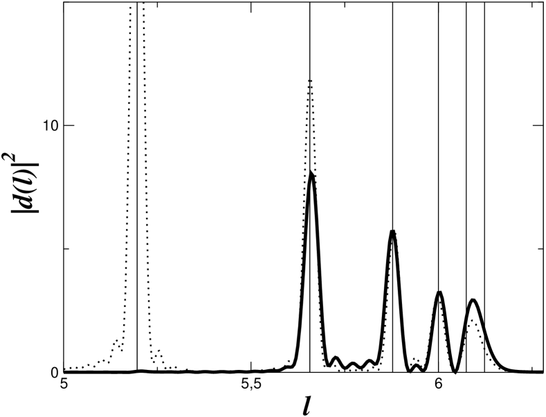
a)

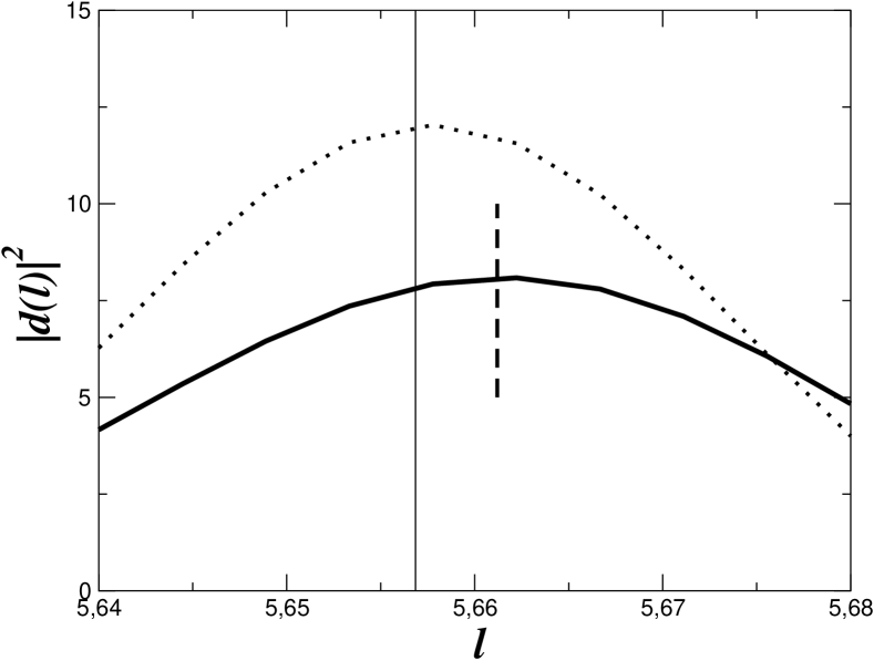
b)

Figure 4: (a) Solid line: length density for dielectric circular cavity with $n=1.5$ and $R=1$. Dotted line: the same but for circular cavity with the Dirichlet boundary conditions. (b) Goos-Hänchen shift associated with the square periodic orbit. Solid line corresponds to the dielectric disk and the dotted line represents the circular closed cavity. Small vertical line indicates the maximum of length spectrum for dielectric disk.

For clarity the dotted line at this figure represents the length density for the closed circular cavity with the Dirichlet boundary conditions. As expected the both models have peaks at periodic orbit lengths but their amplitudes are different. In particular, as for $n=1.5$ the critical angle is of the order of $42^{o}$, triangular periodic orbit is not confined and the corresponding peak for dielectric cavity is practically invisible. Others peaks have similar heights.

VII Corrections to asymptotic regime

According to (25) the contribution of a periodic orbit for an open dielectric cavity differs from a closed cavity only by the value of the total reflection coefficient. Thus, when all incidence angles for a periodic orbit are greater than the critical angle (9), the modulus of its contribution to the trace formula has to be the same as for the closed cavity. The curves at Fig. 4 have been normalized in such a way that their peaks at pentagonal periodic orbit are the same heights. But then the amplitudes corresponding to the square orbit are clearly different (dielectric cavity peak is of the order of $0.7$ of the close cavity peak) which contradicts the above prediction.

Other important corrections are the so-called Goos-Hänchen shift g_h , lai ; martina which manifests itself as a slight difference of a visible length from its geometric length for an orbit reflected from a dielectric interface and the Fresnel filtering fresnel_filt , which manifests itself as a slight shift of the angle of emission near the critical angle for a dieletric boundary. At Fig. 4b) a region of Fig. 4a) close to the maximum of the length density around the square periodic orbit is magnified. The peak of the close cavity represented by dotted line is, as expected, centered at the geometric length of this orbit ($l=4\sqrt{2}R\simeq 5.6568$ for $R=1$). But the peak associated with the dielectric circular cavity is clearly shifted to the right. Numerically, this shift is small and for the considered interval of momentum it is of the order of $0.004R$.

The reason of these discrepancies is related with the fact that asymptotics of the Hankel function (73) is not valid when $m$ is close to $x$ (see e.g. bateman ). The uniform approximation for large $m$ and all $x$ is more complicated and is given e.g. by the Langer formula bateman

$$H_{m}^{(1)}(x)=\left(1-\frac{\arctan\,\omega}{\omega}\right)^{1/2}H_{1/3}^{(1)}(z)\mathrm{e}^{\mathrm{i}\pi/6}+\mathcal{O}(m^{-4/3})$$ (88)

where $z=m(\omega-\arctan\,\omega)$ and $\omega=\sqrt{x^{2}/m^{2}-1}$.

Non-uniform character of this expression is clearly seen from the following asymptotics useful for further estimations

$$\frac{H_{m}^{(1)\prime}(x)}{H_{m}^{(1)}(x)}|_{x=m} = \frac{\alpha}{m^{1/3}}+\mathcal{O}\left(\frac{1}{m}\right)\ ,$$ (89)

$$\frac{\partial}{\partial m}\frac{H_{m}^{(1)\prime}(x)}{H_{m}^{(1)}(x)}|_{x=m} = \frac{\alpha^{2}}{m^{2/3}}+\mathcal{O}\left(\frac{1}{m^{4/3}}\right)$$ (90)

$$\frac{\partial^{2}}{\partial m^{2}}\frac{H_{m}^{(1)\prime}(x)}{H_{m}^{(1)}(x)}|_{x=m} = \frac{2\alpha^{3}-2}{m}+\mathcal{O}\left(\frac{1}{m^{5/3}}\right)$$ (91)

where $\alpha=2^{-2/3}3^{5/6}\pi^{-1}\Gamma^{2}(2/3)\mathrm{e}^{2\pi\mathrm{i}/3}\simeq-.4592+.7954\mathrm{i}$.

To calculate carefully higher order corrections to the trace formula (85) is not an easy task. The main difficulty lies in the fact that the stationary phase method on which trace formulas are based on cannot, strictly speaking, be applied when a periodic orbit has incident angles close to the critical one. The point is that in the stationary phase method it is implicitly assumed that non-exponential terms are changed much slowly than the action in the exponent. This is the case for the usual billiard systems where the whole perturbation series for the trace formula has been constructed gaspard_alonso , vattay .

But as follows from (88) for dielectric cavities exact reflection coefficient (69) near the critical angle changes at a scale of $\delta\bar{m}\sim x^{1/3}$ but the action changes at a different scale of the order of $\delta\tilde{m}\sim x^{1/2}$.

When $x\to\infty$ the former is much smaller than the latter and the stationary phase method when a trajectory hits a boundary with angle close to the critical one can not be justified. To avoid this difficulty one can use the Langer approximation (88) in the transitional region and tabulate the integrals without other approximations. We will not perform these computations here. Instead, we compare the saddle point result with numerically calculated integral for the square and pentagonal periodic orbits. For refractive index $n=1.5$ incident angles of the square periodic orbit are close to the critical angle but for the pentagonal orbit they are far apart and the difference of these two cases will give the accuracy of the pure saddle point results.

From (67) it follows that the full contribution of a periodic orbit with fixed numbers $M$ and $r$ is given by the integral

$$d_{p}(E)=\mathrm{e}^{\mathrm{i}[nkl_{p}-r\pi/2+\pi/4]}J_{M,r}(x)$$ (92)

where

$$J_{M,r}(x)=\frac{R^{2}}{\pi^{2}x^{2}}\int_{-\infty}^{\infty}P_{m}(x)[R_{m}^{(\mathrm{e})}(x)]^{r}E_{m}^{r}(x)$$

$$\times\mathrm{e}^{-\mathrm{i}[nkl_{p}-r\pi/2+\pi/4]}\mathrm{d}m$$ (93)

In the pure stationary phase approximation integral (93) equals

$$J_{M,r}^{(sp)}(x)=\frac{R^{2}}{\pi^{2}x^{2}}P_{m_{sp}}(x)[R_{m_{sp}}^{(\mathrm{e})}(x)]^{r}\sqrt{\frac{2\pi}{g_{2}}}$$ (94)

which in the semiclassical limit tends to

$$J_{M,r}^{(scl)}(x)=\frac{n^{3/2}\mathcal{A}_{p}}{\pi\sqrt{2\pi kl_{p}}}R_{p}^{r}$$ (95)

as in (85).

At the first sight it seems that a better approximation consists in the calculation of the prefactor (72) and the reflection coefficient (69) in (94) directly at the saddle point (80) without the asymptotic formula (73). Roughly speaking, this is equivalent to use for the reflection on a curved surface instead of the Fresnel diffraction coefficient (8) valid for an infinite plane interface the reflection coefficient (69) computed at the saddle point value of the incidence angle $\theta$ as in (87). When this angle is close to the critical angle from (69) one gets

$$R_{m}(\theta,x)=\dfrac{n\cos\theta+\mathrm{i}H_{m}^{(1)\prime}(x)/H_{m}^{(1)}(x)}{n\cos\theta-\mathrm{i}H_{m}^{(1)\prime}(x)/H_{m}^{(1)}(x)}$$ (96)

where the value of the angular momenta $m=m(\theta)$ is related with angle $\theta$ as it follows from the saddle point relation (80)

$$m(\theta)=nx\sin\theta\ .$$ (97)

This type of modification first has been proposed in martina .

Nevertheless, we found that this approximation numerically is not better than the simple semiclassical formula (95). This is because the effective reflection coefficient (96) changes too quickly close to critical angle. Therefore, when a region which gives a dominant contribution to the integral (93) is close but not equal to the saddle point in the exponent, expression (94) differs considerably from the correct one. For this reason we prefer to compare numerical values of the integral (93) not with (94) but with simpler expression (95).

At Fig. 5 the results of numerical calculations of the integral (93) for square and pentagonal periodic orbits are presented. At Fig. 5a) the square of the modulus of this integral divided by the semiclassical expression (95) is given. As expected, contribution of the pentagonal periodic orbit is well described by semiclassical formula. But the contribution of the square periodic orbit differs considerably from the asymptotic result which explains quantitatively the observed differences of the square orbit heights for closed and dielectric cavities seen at Fig. 4.

a)

b)

Figure 5: (a) Modulus square of the integral (93) divided by its semiclassical expression (95). Solid line indicates the contribution of the square periodic orbit. Dashed line is the contribution of pentagonal orbit. (b) The derivatives of the phase of the same integral: solid and dashed lines correspond respectively to the square and pentagonal orbits.

The computed corrections permit also to explain the analog of the Goos-Hänchen shift observed at Fig. 4b). Let us write the periodic orbit contribution in the form

$$d_{p}(E)=|d_{p}(E)|\mathrm{e}^{\mathrm{i}[knl_{p}-r\pi/2+\pi/4+\Psi_{p}(x)]}$$ (98)

where the phase $\Psi_{p}(x)$ comes from the integral (93).

To compute the length spectrum one has to calculate the Fourier harmonics of this expression (32). The shift of the peak position, $\Delta l=l-l_{p}$ can be estimated from the saddle point in the exponent

$$n\frac{\Delta l}{R}=\frac{\partial\Psi_{p}(x)}{\partial x}\ .$$ (99)

At Fig. 5b) the value of this derivative computed numerically from the knowledge of (93) is plotted for the square and pentagonal orbits. For the square orbit its value is larger than for pentagonal one and is of the same order as the observed shift in Fig. 4b). As we are looking for a very small effect, mutual influence of different periodic orbits has to be taken into account when a precise determination of the Goos-Hänchen shift is required.

VIII Conclusion

The goal of the paper is the construction of the trace formula for open dielectric cavities. By using the Krein formula it was demonstrated that such trace formula can be written in the form (30)

$$- \frac{1}{\pi}\sum_{m}\dfrac{\mathrm{Im\ }E_{m}}{(k-\mathrm{Re}\,E_{m})^{2}+(\mathrm{Im}\,E_{m})^{2}}$$ (100)

$$= \bar{d}(E)+\sum_{p}\big{(}d_{p}(E)+d_{p}^{*}(E)\big{)}$$

where in the left-hand side the sum is taken over all internal resonances and in the right-hand side the summation includes all periodic orbits for the free motion inside the cavity. The term $\bar{d}(E)$ is the mean density of these resonances given by the derivative of (27). Its two main terms are

$$\bar{d}(E)=\frac{An^{2}}{4\pi}+\tilde{r}(n)\frac{L}{8\pi k}$$ (101)

where $k=\sqrt{E}$, $A$ and $L$ are the area and the perimeter of the cavity, and $\tilde{r}(n)$ is as follows

$$\tilde{r}(n)=1+\frac{n^{2}}{\pi}\int_{-\infty}^{\infty}\frac{\mathrm{d}t}{t^{2}+n^{2}}R(t)-\frac{1}{\pi}\int_{-\infty}^{\infty}\frac{\mathrm{d}t}{t^{2}+1}R(t)$$ (102)

where $R(t)$ is the reflection coefficient at imaginary momentum defined in (29). Terms related with $R(t)$ correspond to the reflections from inside and outside the boundary but $1$ in (102) appears due to the necessity of removing the $\mathbf{S}$-matrix for the scattering on the cavity with the Dirichlet boundary conditions.

The contribution from a particular periodic orbit, $d_{p}(E)$, to the trace formula (100) differs from the same closed billiard only by the product over Fresnel reflection coefficients (8) computed at all reflection points as in (24) for isolated orbits or their average over a periodic orbit family as in (25).

We have discussed also corrections to the above asymptotic semiclassical formulas. Due to rapid changes of the reflection coefficient close to the critical angle corrections for dielectric cavities are larger than for closed cavities. In particular, higher order corrections permit to estimate the analog of the Goos-Hänchen shift for the peak position in dielectric cavity length density.

Obtained formulas were compared with numerical calculation of resonances for the circular dielectric cavity and in all cases a good agreement was observed.

Appendix A Krein formula for one dimensional systems

To illustrate the Krein formula in the simplest case of a one-dimensional system consider a particle moving along the positive half-axis in a potential without bound states. For simplicity, assume that (i) $\psi(0)=0$ and (ii) the potential is zero for distances larger than $a$. The corresponding quantum problem has only continuous spectrum. To get artificially the discrete spectrum let us impose that at some large distance $R\gg a$ the wave function obeys

$$\psi(R)=0\ .$$ (103)

Eigenfunctions of a such system at large distances $x>a$ have the form of plane waves

$$\psi(x)\propto\sin(kx+\delta(E)),$$ (104)

where $k=\sqrt{E}$ and the phase shift $\delta(E)$ contains all information about the potential.

Eigenmomenta, $k_{m}$, of this system are determined from the condition (103) and they read

$$k_{m}R+\delta(E)=\pi m$$ (105)

where integer $m$ counts the number of states. By definition, the density of states, $d(E)$, is the number of states within an interval $\mathrm{d}E$

$$d(E)\equiv\frac{\mathrm{d}m}{\mathrm{d}E}=\frac{R}{2\pi\sqrt{E}}+\frac{1}{\pi}\frac{\partial\delta(E)}{\partial E}\ .$$ (106)

But the function (104) with $\delta(E)=0$ is the eigenfunction of the free problem without the potential. Therefore, the first term in the last equation describes the free density of states

$$d_{0}(E)=\frac{R}{2\pi\sqrt{E}}\ .$$ (107)

The excess density due to the presence of the potential is the difference between the level density with the potential and without it. From (106) it follows that

$$d(E)-d_{0}(E)=\frac{1}{\pi}\frac{\partial\delta(E)}{\partial E}\ .$$ (108)

Instead of the phase shift it is instructive to introduce the $\mathbf{S}$-matrix for the scattering on the potential defined as the ratio of the amplitude of the outgoing wave to the amplitude of the incoming wave. For the function (104) one has

$$\mathbf{S}(E)=-\mathrm{e}^{2\mathrm{i}\delta(E)}\ .$$ (109)

Therefore, the excess density of states reads

$$d(E)-d_{0}(E)=\frac{1}{2\pi\mathrm{i}}\frac{\partial\ln\mathrm{S}(E)}{\partial E}\ ,$$ (110)

which is the 1-dimensional version of the Krein formula (17).

It is also straightforward to compute explicitly all necessary quantities for a 1-dimensional dielectric cavity these_Melanie . Consider a dielectric segment of size $L$ with the refractive index $n$ in a media with the refractive index $1$ as at Fig. 6.

Figure 6: 1-dimensional dielectric cavity. Refractive indices are indicated above the axis.

After imposing condition (103) one gets that the density of states $d(E)$ has to be determined from the formula

$$d(E)=-\frac{1}{\pi}\int_{0}^{R}\mathrm{Im\ }n^{2}(x)G(x,x)\mathrm{d}x$$ (111)

where $n(x)=n$ inside the cavity and $n(x)=1$ outside it, and $G(x,y)$ is the Green function of our problem these_Melanie . Using

$$d_{0}(E)=-\frac{1}{\pi}\int_{0}^{R}\mathrm{Im\ }G^{(0)}_{k}(x,x)\mathrm{d}x=\frac{R}{2\pi k}$$ (112)

where $G^{(0)}(x,y)=\mathrm{e}^{\mathrm{i}k|x-y|}/2\mathrm{i}k$ is the free Green function after some calculations one finds that for antisymmetric states when $R\to\infty$

$$d(E)-d_{0}(E)=-\frac{L}{2\pi k}+\frac{nL}{2\pi k}\frac{1-r^{2}}{|1+r\mathrm{e}^{2\mathrm{i}nkL}|^{2}}\$$ (113)

where $r$ is the Fresnel reflection coefficient from dielectric boundary

$$r=\frac{n-1}{n+1}\ .$$ (114)

Correspondingly, the $\mathbf{S}$-matrix for antisymmetric states is

$$\mathbf{S}(E)=-\mathrm{e}^{2\mathrm{i}(n-1)kL}\frac{1+r\mathrm{e}^{-2\mathrm{i}nkL}}{1+r\mathrm{e}^{2\mathrm{i}nkL}}\ ,$$ (115)

which, of course, agrees with 1-dimensional Krein formula (110). This $\mathbf{S}$-matrix has an infinite number of poles (or resonances) corresponding to the solutions of the equation $1+r\mathrm{e}^{2\mathrm{i}nk_{m}L}=0$ or explicitly

$$k_{m}=\frac{\pi}{nL}(m+\frac{1}{2})-\frac{\mathrm{i}}{2nL}\ln\frac{n+1}{n-1}$$ (116)

where $m$ is an integer.

Using the identity

$$\frac{1-r^{2}}{1+r^{2}+2r\cos(x)}=\sum_{j=-\infty}^{\infty}(-r)^{|j|}\mathrm{e}^{\mathrm{i}jx}$$ (117)

valid for $|r|<1$ one can rewrite (113) as the trace formula for resonances in the considered simplest case

$$\frac{1}{\pi}\sum_{m=\infty}^{\infty}\frac{\mathrm{Im}k_{m}}{(k-\mathrm{Re}k_{m})^{2}+(\mathrm{Im}k_{m})^{2}}$$

$$=\frac{nL}{2\pi k}\sum_{j=-\infty}^{\infty}(-r)^{|j|}\mathrm{e}^{2\mathrm{i}jnLk}\ .$$ (118)

The term with $j=0$ in this equation corresponds to the mean density of resonances and terms with $j\neq 0$ describe the contributions from the unique primitive periodic orbit and its repetitions.

Notice that the transition from the Krein formula (113) to the trace formula (118) is done by removing from the $\mathbf{S}$-matrix (115) the factor $\mathbf{S}_{0}(E)=-\mathrm{e}^{-2\mathrm{i}kL}$ which is exactly the $\mathbf{S}$-matrix for the scattering on the same cavity but with the Dirichlet boundary condition at the right end of the cavity $x=L$. This is the same phenomenon as for the circular dielectric cavity discussed in Section 3.

References

- (1) R. Balian, C. Bloch, Ann. Phys. 60, 401 (1970); Ann. Phys. 64, 271 (1971); Ann. Phys. 69, 76 (1972)
- (2) M. Gutzwiller, J. Math. Phys. 12, 343 (1971)
- (3) M. Gutzwiller, Chaos in Classical and Quantum Mechanics, Springer (1990)
- (4) M. V. Berry, M. Tabor, Proc. Roy. Soc. Lond. 349, 101 (1976)
- (5) P. Gaspard, Chaos, scattering and statistical mechanics, Cambridge University Press (1998)
- (6) P. Cvitanovic and B. Eckhardt, Phys. Rev. Lett. 63, 823 (1989)
- (7) J.U. Nöckel and A.D. Stone, Nature 385, 45 (1997)
- (8) C. Gmachl, F. Capasso, E.E. Narimanov, J.U. Nöckel, A.D. Stone, J. Faist, D.L. Sivco, and A.Y. Cho, Science 280, 1556 (1998)
- (9) M. Lebental, N. Djellali, C. Arnaud, J.-S. Lauret, J. Zyss, R. Dubertrand, C. Schmit, E. Bogomolny, Phys. Rev. A, 76, 023830 (2007)
- (10) M. Lebental, Quantum chaos and organic microlasers, PhD thesis (2007)
- (11) T. Fukushima, T. Harayama, J. Wiersig,Phys. Rev. A, 73, 023816 (2006)
- (12) M.G. Krein, Matem. Sbornik 33, 597 (1953); Dokl. Akad. Nauk, SSR 144, 268 (1962); English trans. in Soviet Math. Dokl. 3 (1962)
- (13) F. Goos and H. Hänchen, Ann. Phys. 1, 333 (1947); K. Artman, Ann. Phys. 2, 87 (1948); Ann. Phys. 8, 270 (1951)
- (14) E. Bogomolny et al. Trace formula for dielectric cavities: II. Polygonal and chaotic cavities, in preparation (2008)
- (15) J.D. Jackson, Classical electrodynamics, 3rd ed., Wiley, New York, 1998
- (16) R. Dubertrand, E. Bogomolny, N. Djellali, M. Lebental and C. Schmit, Phys. Rev. A, 77, 013804 (2008)
- (17) L. B. Felsen, N. Marcuvitz, Radiation and scattering of waves, IEEE Press Series, New York (1994)
- (18) R.G. Newton, Scattering theory of waves and particles, Second ed., Springer-Verlag, New York (1982)
- (19) A.D. Rawlings, IMA J. Appl. Math. 19, 261 (1977)
- (20) I.M. Lifshitz, Uspekhi Mat. Nauk, 7, 171 (1952)
- (21) M.Sh. Birman and D.R. Yafaev, Algebra i analysiz, 4 (1992); English transl. in St. Petersburg Math. J. 4, 833 (1993)
- (22) M. Zworski, Asian J. Math. 2, 609 (1998)
- (23) M. Zworski, Séminaire E.D.P. 1996-1997, École Polytechnique, XIII-1-XIII-12
- (24) J. Main, J. Wiersig,Phys. Rev. E, 77, 036205 (2008)
- (25) J. Sjöstrand and M. Zworski, Journal of AMS, 4, 729 (1991)
- (26) W. Lu, S. Sridhar, and M. Zworski, Phys. Rev. Lett. 91, 201 (2003)
- (27) S. Nonnenmacher and E. Schenck, ArXiv: 0803.1075 [nlin-CD].
- (28) E. Bogomolny, N. Pavloff, and C. Schmit, Phys. Rev. E 61, 3689 (2000)
- (29) G. Vattay, A. Wirzba, and P.E. Rosenqvist, Phys. Rev. Lett. 73, 2307 (1994)
- (30) Higher transcendental functions, A. Erdelyi Ed., Vol. II, McGraw-Hill Book Company, New York, Toronto, London, (1955)
- (31) P. Debije, Physik. Zeitschrift 22,9, 775 (1908).
- (32) T. Harge et G. Lebeau, Invent. Math. 118, 161 (1994)
- (33) J. Sjöstrand and M. Zworski, Arx. Mat. 33, 135 (1995)
- (34) A. Martinez, Ann. Henri Poincaré 4, 739 (2002)
- (35) U. Smilansky and I. Ussishkin, J. Phys. A: Math. Gen. 29, 2587 (1996)
- (36) H.M. Lai, F.C. Cheng, and W.K. Tang, J. Opt. Soc. Am. 3, 550 (1986)
- (37) M. Hentschel and H. Schomerus, Phys. Rev. E 65, 045603 (2002)
- (38) H. E. Tureci, A. D. Stone,Opt. Lett.,27, 7 (2002)
- (39) P. Gaspard and D. Alonso, Phys. Rev. A 47, R3468 (1993)
- (40) G. Vattay and P.E. Rosenqvist, Phys. Rev. Lett. 76, 335 (1996)