Physical and kinematical properties of the X-ray absorber in the broad absorption line quasar APM 08279+5255

Abstract

Context. We have re-analyzed the X-ray spectra of the gravitational lensed high-redshift BAL QSO APM 08279+5255, observed with the XMM-Newton and Chandra observatories. Previous studies (Hasinger et al. 2002; Chartas et al. 2002) detected unusual, highly-ionized iron absorption features, but differed in their interpretation of these features, regarding the kinematical and ionization structure.

Aims. We seek one physical model that can be successfully applied to both observations.

Methods. For the first time we have performed detailed photoionization modeling on the X-ray spectrum of APM 08279+5255.

Results. The absorbing gas in APM 08279+5255 can be represented by a two-absorbers model with column densities $N_{H}(1)\approx 7\times 10^{22}$ ${\rm cm}^{-2}$, $N_{H}(2)\approx 6\times 10^{22}$ ${\rm cm}^{-2}$, and ionization parameters $\log\xi(1)\approx 1.5$ and $\log\xi(2)\approx 3$, with one of them (the high-ionization component) outflowing at $v\approx 0.18(\pm 0.01)c$, carrying large amount of gas out of the system. We find that the Chandra spectrum of APM 08279+5255 requires the same Fe/O ratio overabundance (previously) indicated by the XMM-Newton observation, showing that both absorber components underwent similar chemical evolution and/or have similar origin.

1 Introduction

Broad absorption line (BAL) quasi-stellar objects (QSOs) are objects displaying in their spectra broad (FWHM $\approx$ 10 000 km ${\rm s}^{-1}$) absorption lines in the rest-frame ultraviolet (UV), originated in outflows of matter from the central engine of QSOs (Foltz et al. 1990; Weymann et al. 1991). The outflow velocity may reach up to $0.2c$ (e.g., Foltz et al. 1983). Determining the relationship between the material absorbing the X-rays and the one absorbing the UV radiation is key to our understanding of the geometry and the physical state of the medium surrounding the vicinity of supermassive black holes (e.g., Mathur et al. 1995; Murray et al. 1995; Hamann 1998; Proga et al. 2000).

Before Chandra/XMM-Newton missions, detections of BAL quasars in X-ray were rare. Usually, these object are X-ray weak (e.g., Gallagher et al. 2006), sometimes interpreted as strong excess absorption. Chandra and XMM-Newton observations of BAL QSOs, have provided new constraints in the amount of absorption toward selected objects (e.g., Sabra & Hamann 2001; Oshima et al. 2001; Gallagher et al. 2002, 2006), indicating large column densities $N_{H}\gtrsim 10^{23}$ ${\rm cm}^{-2}$.

The BAL QSO APM 08279+5255 at redshift $z=3.91$ (Irwin et al. 1998) is one of the most luminous objects in the universe, further magnified by gravitational lensing by a factor of $\sim 50-100$ (e.g., Ledoux et al. 1998). It was detected with the Submilimiter Common-User Bolometric Array, implying an apparent far-infrared luminosity greater than 5$\times 10^{15}L_{\sun}$ (Lewis et al. 1998). The optical spectrum, obtained with the High Resolution Echelle Spectrometer at the Keck telescope (Ellison et al. 1999), along with a detailed study of the physical conditions in the BAL flow of the QSO by Srianand & Petitjean (2000), allowed them to conclude that the corresponding gas stream, outflowing with velocities of up to 12 000 km ${\rm s}^{-1}$, is heavily structured and highly ionized.

The quasar APM 08279+5255 was observed twice with XMM-Newton (Hasinger et al. 2002, hereafter H02). In both observations the quasar is observed clearly out to 12 keV, which corresponds to almost 60 keV in the rest frame. The most apparent feature in the XMM-Newton spectrum is an absorption-like feature around 1.55 keV (which they interpret as an absorption edge), corresponding to $\sim 7.7$ keV in the rest frame of APM 08279+5255. The high-inferred iron abundance at the high redshift, corresponding to a young age of the universe, is of great interest in the context of chemical enrichment models, and provides constraints on the early star formation history of the universe and on its cosmological parameters (e.g., Hamann & Ferland 1993; Hasinger et al. 2002; Komossa & Hasinger 2003).

The quasar APM 08279+5255 was also observed with Chandra (Chartas et al. 2002, hereafter C02). The Chandra spectrum shows a similar absorption feature as the XMM-Newton observation, but the feature led to a different interpretation. In particular, C02 modeled the spectrum with two absorption lines at 8.1 keV and 9.8 keV in the rest frame of the quasar, interpreted as Fe xxv K lines. If the Chandra interpretation of the data is right, the bulk velocity of the X-ray BALs is $\sim 0.2c-0.4c$. The presence of similar outflow velocities has been claimed in a few other AGN X-ray spectra (e.g., Pounds et al. 2003; Chartas et al. 2003; Pounds & Page 2006), but alternative interpretations of the same spectra have been proposed, which do not require these relativistic outflow velocities (e.g., Kaspi & Behar 2006).

New models (e.g., Elvis 2000; Proga et al. 2000; Proga 2007) predict that a large fraction of the accreted matter into the region of the compact object, is expelled out again in the form of high-velocity outflows. Broad UV absorption features, with velocities $\sim$ 0.05$c-0.1c$, are associated with this material through acceleration mechanisms like acceleration by gas pressure (e.g., Weymann et al. 1982; Begelman et al. 1991) due to dust (e.g., Voit et al. 1993; Yun & Scoville 1995) and acceleration due to radiative pressure by spectral lines (e.g., Drew & Boksenberg 1984; Shlosman et al. 1985; Arav et al. 1994; de Kool & Begelman 1995; Murray et al. 1995; Proga et al. 2000) observed in about 10% of luminous high-$z$ quasars (Laor & Brandt 2002), implying that these outflows are an important component of the general picture of AGNs. Furthermore, these models also predict that in order for the UV material to reach such high velocities a shield made by a high column density of gas ($N_{H}\sim 10^{22}-10^{24}$ ${\rm cm}^{-2}$) must absorb radiation in the X-ray band, in this manner preventing the destruction of the UV material. The new generation of X-ray observatories, XMM-Newton and Chandra give us an unique opportunity to study in detail the X-ray component of the BAL QSOs, contributing in our knowledge about the dynamical and physical evolution of the center of these systems, and in the case of high-redshited BAL QSOs, the gas enrichment history in the early universe (Hamann et al. 2004).

However, none of the previous studies include a self-consistent photoionization modeling of the X-ray spectrum of APM 08279+5255. Any constraint on the ionization level of the absorbing gas and its connection with the kinematical properties of the BAL outflow is of major interest to elucidate some of the greatest discrepancies between these two proposed models. Furthermore, a model that can separate the differences between observations (XMM-Newton vs Chandra), or unify both in a single frame, is highly desirable. We report a spectral analysis (made of these two observations separated by $\sim 2$ weeks in the rest frame) of the high-redshifted BAL QSO APM 08279+5255, and present one model that might reconcile both observations in the same physical context, shedding new light on the ionization degree, kinematics and evolution of this system, in connection with its cosmological consequences. We use the following cosmological parameters: H${}_{0}=70$ km ${\rm s}^{-1}$ Mpc^-1, $\Omega_{M}=0.3$ and $\Omega_{\lambda}=0.7$.

2 X-ray observations and Spectral analysis

The quasar APM 08279+5255 was observed twice with XMM-Newton. The first X-ray observation was made on 2001 October 30 with $\sim 15$ ks of exposure time (referred as XMM1 in Table 2 of H02). A significantly longer ($\sim 100$ ks) observation was made in 2002 April 28$-$29 (referred as XMM2 in Table 2 of H02). Taking advantage of the improvement in calibration and effective areas used in XMM-Newton observations, we re-processed the primary event file and extracted the spectrum, using the most updated XMM-Newton Science Analysis System (SAS, version 7.0.0), and the standard data pipeline processing. In our analysis, we used the $\sim 88.8$ ks Chandra ACIS-I observation of APM 08279+5255 (see Table 1 of C02), and extracted the spectrum, built ancillary and redistribution matrix files with CIAO version 3.4. Details on calibration fluxes and count rates can be found in the respective works.

We will present the spectral analysis in three steps: 1) By showing results from C02 (below in this section), 2) comparing them with H02 (below in this section), and 3) we introduce our own approach highlighting the differences between these sets of data (XMM-Newton vs Chandra, in Sect. 3). Then we proceed to three more steps: 1) fitting the edge and line models; 2) fitting photoionization models to the XMM-Newton and Chandra data separately; and 3) fitting jointly in the context of one consistent model (in Sect. 4).

In C02, the authors are able to fit an absorbed power-law with an intrinsic neutral absorber in the frame of the quasar, to the Chandra spectrum of APM 08279+5255. They find a best-fit photon index $\Gamma\approx 1.7$ and the column density of the absorber $N_{H}\approx 6\times 10^{22}$ ${\rm cm}^{-2}$. Significant residuals are found at $\sim 8$ keV (rest-frame). This is the source of an important controversy. By the time C02 was under review, the authors had published H02, in which a good description of the spectrum is proposed by fitting a model that included an absorption edge (zphabs $\times$ Pl $\times$ 1-Edge or Edge model) at $\sim 8$ keV to the XMM-Newton observation of this object. Despite the fact that Chandra data provides values for the parameters for the Edge model, its $\chi_{\nu}^{2}$ is statistically poor ($\sim 1.36$ for 107 degrees of freedom [d.o.f]). Moreover, C02 tried to model this feature with a Single-Gaussian line model (the one at $\sim$ 8.1 keV) and the fit gets a bit worse ($\chi_{\nu}^{2}\sim 1.41$ for 106 d.o.f). They found a better fit with a Two-Gaussian lines model at $\sim 8.1$ keV and $\sim 9.8$ keV (rest frame), which indeed significatively improved the description of the data over the Edge model. A visual comparison between the two sets of data suggests that the absorption feature is present in both cases, but the line-shape of the feature appears to be weakened in the XMM-Newton observation.

As noted by H02, a major improvement (in the description of the XMM-Newton spectrum of APM 08279+5255) is found by adding an absorption edge to the absorbed power-law (Fit 2 in Table 1). Our best-fit model for the XMM-Newton data provides an edge energy at $\approx$ 7.7 keV (in the rest frame) and an optical depth $\tau\approx 0.3$. This was interpreted by the previous authors as a Fe edge, compatible with ionization potentials of iron from Fe xv to Fe xviii, implying a significant ionization of iron. Indeed, in that work the authors compared the absorption seen in the spectrum at low-energies and arrived at the conclusion that an overabundance of iron ($\sim 2-5$) with respect to lower $Z$ elements (O, Ne, Mg, Si and S) is necessary to account for this feature ($N_{\rm Fe}\approx 1.5\times 10^{19}$ ${\rm cm}^{-2}$).

In all our fits, we have included a neutral absorption with the Galactic value fixed to $N_{H}=3.9\times 10^{20}$ ${\rm cm}^{-2}$ (Stark et al. 1992). We begin our spectral analysis by fitting an absorbed power-law with an intrinsic neutral absorber in the frame of the quasar ($z=3.91$). Our XMM (EPIC pn+MOS) and XMM EPIC pn data (Strüder et al. 2001), are consistent with each other and with the Chandra fit (included also the H02 fits for comparison purposes). The photon index is $\Gamma\sim 1.7-2$ and the column density of the absorber is $N_{H}\sim 6\times 10^{22}$ ${\rm cm}^{-2}$. Table 1 quotes the parameter values of the model along with the goodness-of-fit in terms of a global $\chi^{2}$ for the d.o.f used for each dataset (bins included in the range $0.2-10$ keV minus the number of free parameters of the model), and the global $\chi^{2}-$probability ($P_{\nu,\chi^{2}}$), which gives the probability of exceeding $\chi^{2}$ for $\nu$ degrees of freedom. Additionally, we introduce a criterion to assess the fits close to the absorption feature, thus we take the global parameters of the model and compute $\chi^{2}$ in the band $(1-2)$ keV (observed frame), along with its corresponding local $\chi^{2}-$probability.

Table 1: Fit Results and comparison between sets of data. XMM-Newton vs Chandra observations of APM 08279+5255.

Parameter	H a	C b	(pn+MOS)c	pnd	Cne
Fit 1: Pl and Neutral Absorption at Source
$\Gamma$	$2.04_{-0.03}^{+0.03}$	$1.72_{-0.06}^{+0.03}$	$1.99_{-0.02}^{+0.02}$	$2.05_{-0.03}^{+0.03}$	$1.79_{-0.03}^{+0.03}$
Normf	$1.30_{-0.05}^{+0.05}$		$1.23_{-0.02}^{+0.02}$	$1.25_{-0.02}^{+0.02}$	$1.02_{-0.02}^{+0.02}$
$N_{H}$ ($\times 10^{22}$ ${\rm cm}^{-2}$)	$6.92_{-0.32}^{+0.32}$	$6.0_{-0.8}^{+0.8}$	$5.95_{-0.21}^{+0.21}$	$6.28_{-0.25}^{+0.26}$	$7.18_{-0.38}^{+0.41}$
$\chi^{2}$/(d.o.f)	481.8/(365)	182.1/(109)	564.5/(478)	330/(290)	229.7/(184)
$P_{{\rm global}}[{\rm Fit\leavevmode\nobreak\ 1}]$	$2\times 10^{-5}$	$1.5\times 10^{-5}$	$3\times 10^{-3}$	0.05	0.01
$\chi^{2}(1-2\leavevmode\nobreak\ {\rm keV})$/(d.o.f)	…	…	134.7/(59)	72.4/(35)	85.7/(52)
$P_{(1-2\leavevmode\nobreak\ {\rm keV})}[{\rm Fit\leavevmode\nobreak\ 1}]$	…	…	$2\times 10^{-9}$	$6\times 10^{-5}$	$2\times 10^{-3}$
Fit 2: Pl and Neutral Absorption at Source, and One Edge
$\Gamma$	$2.01_{-0.03}^{+0.03}$		$1.96_{-0.02}^{+0.02}$	$2.02_{-0.03}^{+0.03}$	$1.77_{-0.02}^{+0.02}$
Normf	$1.37_{-0.06}^{+0.06}$		$1.28_{-0.02}^{+0.02}$	$1.31_{-0.02}^{+0.02}$	$1.09_{-0.01}^{+0.01}$
$N_{H}$ ($\times 10^{22}$ ${\rm cm}^{-2}$)	$7.34_{-0.34}^{+0.34}$		$6.20_{-0.21}^{+0.22}$	$6.54_{-0.26}^{+0.27}$	$7.50_{-0.24}^{+0.25}$
$E_{\rm edge}$ (keV)	$7.68_{-0.10}^{+0.10}$	$7.68_{-0.25}^{+0.21}$	$7.70_{-0.17}^{+0.16}$	$7.53_{-0.19}^{+0.21}$	$7.70_{-0.13}^{+0.11}$
$\tau$	$0.46_{-0.05}^{+0.05}$	$0.37_{-0.13}^{+0.14}$	$0.30_{-0.06}^{+0.06}$	$0.33_{-0.07}^{+0.08}$	$0.38_{-0.05}^{+0.05}$
$\chi^{2}$/(d.o.f)	394.6/(362)	146/(107)	506/(476)	292/(288)	190.1/(182)
$P_{{\rm global}}[{\rm Fit\leavevmode\nobreak\ 2}]$	0.12	$6\times 10^{-3}$	0.17	0.44	0.35
$\chi^{2}(1-2\leavevmode\nobreak\ {\rm keV})$/(d.o.f)	…	…	74.5/(59)	35.4/(35)	53.7/(52)
$P_{(1-2\leavevmode\nobreak\ {\rm keV})}[{\rm Fit\leavevmode\nobreak\ 2}]$	…	…	0.09	0.51	0.46
Fit 3: Pl and Neutral Absorption at Source, and One Gaussian
$\Gamma$	…	$1.73_{-0.06}^{+0.06}$	$1.99_{-0.02}^{+0.02}$	$2.04_{-0.03}^{+0.03}$	$1.80_{-0.02}^{+0.02}$
Normf	…		$1.25_{-0.02}^{+0.01}$	$1.26_{-0.02}^{+0.02}$	$1.06_{-0.01}^{+0.01}$
$N_{H}$ ($\times 10^{22}$ ${\rm cm}^{-2}$)	…	$6.4_{-0.9}^{+0.8}$	$6.04_{-0.20}^{+0.23}$	$6.28_{-0.24}^{+0.27}$	$7.39_{-0.24}^{+0.25}$
$E_{\rm line1}$	…	$8.05_{-0.07}^{+0.18}$	$8.12_{-0.03}^{+0.04}$	$7.97_{-0.03}^{+0.03}$	$8.11_{-0.01}^{+0.01}$
$\sigma_{\rm line1}$	…	<$0.140$	$0.34_{-0.11}^{+0.13}$	$0.15_{-0.06}^{+0.07}$	$0.09_{-0.02}^{+0.02}$
${\rm EW}_{\rm line1}$ (keV)	…	$0.23_{-0.07}^{+0.06}$	$0.14_{-0.11}^{+0.18}$	$0.16_{-0.10}^{+0.22}$	$0.17_{-0.04}^{+0.04}$
$\chi^{2}$/(d.o.f)	…	146.9/(106)	531.3/(476)	310.8/(288)	198.4/(181)
$P_{{\rm global}}[{\rm Fit\leavevmode\nobreak\ 3}]$	…	$5.3\times 10^{-5}$	0.04	0.18	0.35
$\chi^{2}(1-2\leavevmode\nobreak\ {\rm keV})$/(d.o.f)	…	…	98.8/(59)	53.2/(35)	55.29/(52)
$P_{(1-2\leavevmode\nobreak\ {\rm keV})}[{\rm Fit\leavevmode\nobreak\ 3}]$	…	…	$5\times 10^{-4}$	0.03	0.4
Fit 4: Pl and Neutral Absorption at Source, and Two Gaussian
$\Gamma$	…	$1.72_{-0.05}^{+0.06}$	$1.98_{-0.02}^{+0.02}$	$2.03_{-0.03}^{+0.03}$	$1.79_{-0.02}^{+0.02}$
Normf	…		$1.28_{-0.02}^{+0.02}$	$1.29_{-0.02}^{+0.02}$	$1.08_{-0.01}^{+0.02}$
$N_{H}$ ($\times 10^{22}$ ${\rm cm}^{-2}$)	…	$6.7_{-0.8}^{+0.9}$	$6.20_{-0.21}^{+0.22}$	$6.49_{-0.25}^{+0.27}$	$7.47_{-0.25}^{+0.24}$
$E_{\rm line1}$ (keV)	…	$8.05_{-0.08}^{+0.10}$	$8.05_{-0.02}^{+0.02}$	$7.93_{-0.03}^{+0.03}$	$8.09_{-0.01}^{+0.01}$
$\sigma_{\rm line1}$ (keV)	…	<$0.140$	$0.08_{-0.03}^{+0.02}$	$0.09_{-0.04}^{+0.04}$	$0.06_{-0.01}^{+0.01}$
${\rm EW}_{\rm line1}$ (keV)	…	$0.24_{-0.07}^{+0.06}$	$0.24_{-0.07}^{+0.12}$	$0.30_{-0.10}^{+0.15}$	$0.31_{-0.10}^{+0.19}$
$E_{\rm line2}$ (keV)	…	$9.79_{-0.19}^{+0.20}$	$9.53_{-0.08}^{+0.10}$	$9.52_{-0.09}^{+0.10}$	$9.72_{-0.04}^{+0.05}$
$\sigma_{\rm line2}$ (keV)	…	$0.41_{-0.16}^{+0.19}$	$0.80_{-0.20}^{+0.40}$	$0.80_{-0.10}^{+0.30}$	$0.70_{-0.14}^{+0.24}$
${\rm EW}_{\rm line2}$ (keV)	…	$0.43_{-0.13}^{+0.17}$	$0.19_{-0.08}^{+0.10}$	$0.21_{-0.11}^{+0.13}$	$0.22_{-0.09}^{+0.14}$
$\chi^{2}$/(d.o.f)	…	106.7/(103)	509.7/(474)	293.2/(286)	178.9/(179)
$P_{{\rm global}}[{\rm Fit\leavevmode\nobreak\ 4}]$	…	0.41	0.13	0.39	0.52
$\chi^{2}(1-2\leavevmode\nobreak\ {\rm keV})$/(d.o.f)	…	…	75.3/(59)	35.5/(35)	44.8/(52)
$P_{(1-2\leavevmode\nobreak\ {\rm keV})}[{\rm Fit\leavevmode\nobreak\ 4}]$	…	…	0.08	0.51	0.79

All absorption-line and edge parameters are computed for the rest frame. The error parameters are 90% confidence limits. (a) Hasinger et al. (2002) (b) Chartas et al. (2002) (c) The fits are carried out fitting simultaneously the pn+MOS data. 293 PI bins are from the pn data, and 188 bins are from the MOS data (in the range 0.2$-$10 keV). (d) Only pn data. (e) Our reprocessed Chandra data, with 187 bins. (f) Power-law normalization, $\times 10^{-4}$ photons keV^-1cm^-2s^-1 at 1 keV in the observed frame. Pl$\equiv$ Power-law.

We include in this analysis, fits of the XMM-Newton data of the Single and Two-Gaussian models, and the results are presented in Table 1, for two sets of XMM-Newton data. One in which we fit simultaneously the EPIC pn, MOS1 and MOS2 (pn+MOS) data and another only taking the EPIC pn data (pn). In the case of the Single-Gaussian line model, both sets are compatible with each other and with the Chandra fit, and the three sets are in agreement with an absorption feature with equivalent width (EW) $\sim 0.2$ keV. For the Two-Gaussian lines model, the best-fit parameters lead to absorption lines at $\sim 8$ keV and $\sim 9.5$ keV (rest frame) with EW $\sim 0.30$ keV and $\sim 0.20$ keV, respectively (all of them compatible with the Chandra measurements, within the errors). But, in this case, the $\chi^{2}-$probabilities are (for the Chandra fits) higher than those for the Single-Gaussian line model, and the Edge model (with 4 parameters more), in both senses, global and locally. In principle, the fits of both models (Fit 2 and Fit 4) are formally acceptable for both sets of data. A more careful analysis, using physically-motivated arguments is required to elucidate the ambiguity of this issue. A temporal variability study may help to solve some aspect of the problem. We present a brief overview of the variability observed in the X-ray spectrum of APM 08279+5255, as seen from the point of view of the XMM-Newton and Chandra data in the next section. A more quantitative physical discussion is given in Sect. 6.

3 Variability of the absorption structure at $\sim$ 7.7 keV $-$ 8 keV

For this analysis, we worked on two sets of XMM-Newton data; a 16 ks exposure time observation of APM 08279+5255 (XMM1), and a 100 ks exposure time observation (XMM2), see Table 1 of H02. As a first step, we were interested in searching for variability within each observation. We looked at the count rate light curves for XMM1 and XMM2. We see slight changes in the light curve, although almost always within $\sim 10$%, obtaining an average of $\sim 0.17$ cts s^-1 for XMM1 and $\sim 0.13$ cts s^-1 for XMM2. For the rest of the analysis we will only use the data of the XMM2 observation of APM 08279+5255, since it collects one order of magnitude more photons with respect to XMM1, increasing notably the signal-to-noise ratio, and we refer to it as the XMM-Newton data. We also looked for evidence of variability in the Chandra observation of APM 08279+5255, but no significant deviation from the average $\sim 6.6\times 10^{-2}$ cts s^-1 was found, fully compatible with the count rate reported by C02.

Here, we discuss in some detail the differences we are seeing between the XMM-Newton and Chandra observations, which are separated by $\sim 2$ months in observed frame ($\sim 2$ weeks in the frame of the quasar), in the context of best-fit models. To begin with, we will assume that indeed both sets of data are better represented by two different models (Edge model vs 2-Absorption-lines model), and study how the Chandra data (better represented by the 2-Absorption-lines model, see C02 for details) behaves with the best-fit model parameters extracted from fitting procedure, using XMM-Newton data (specifically, the Edge model parameters taken from Table 2 of H02), and vicerversa (i.e., how the XMM-Newton data behaves with the best-fit model parameters found in fits using Chandra data).

First, we applied the simplest strategy: We use $\chi^{2}-$statistics to describe the goodness-of-fit of the data to the model. In Fig. 1 (left panel), we plot the Edge model, taking the intrinsic absorption $N_{H}$, optical depth $\tau$ and energy of the edge from Table 2 of H02, leaving only the normalization and the photon index $\Gamma$ free to vary (all these numbers are fully consistent with our own best-fit parameters, see Table 1).

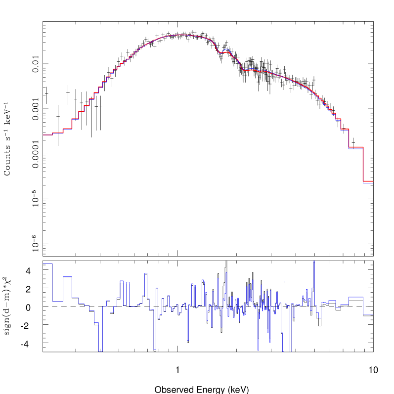
Figure 1: Chandra X-ray spectrum of APM 08279+5255 with two models over-plotted: the Edge model (solid red line) and the 2-Absorption-lines model (solid blue line). In the right panel, we show a closer view of the residuals in the range $1-2$ keV. Solid line is the Edge model. Dashed line is the 2-Absorption-lines model.

The resulting $\chi^{2}$ is 192 for 185 d.o.f. We also plot the 2-Absorption-lines model, but this time we allow all parameters free to vary (all the numbers fully consistent with the parameters reported by C02). This time $\chi^{2}=179$ for 180 d.o.f. At this stage, we are unable to judge which model is better at describing the data, since it is true that the 2-Absorption-lines model reports a smaller $\chi^{2}$, but it also introduces more free parameters in the fitting procedure, which might produce the advantage. A simple hypotheses $F$-test is not permitted under this context, partly because these two are not nested models (a detailed discussion about conditions under which the $F$-test is valid is given in Protassov et al. 2002). Therefore, because the differences between models are actually local, we focused on the spectral discrepancies close to the strongest absorption feature at $\approx 1.6$ keV (observed frame), specifically the range $1-2$ keV. We have adopted both models using the global best-fit parameters, but evaluate $\chi^{2}$ locally from 1 to 2 keV. The results are: $\chi^{2}[{\rm Edge}]_{(1-2\leavevmode\nobreak\ {\rm keV})}=55$ and $\chi^{2}[{\rm 2Lines}]_{(1-2\leavevmode\nobreak\ {\rm keV})}=45$ for 52 d.o.f. First, it is easy to see that the differences between globals $\chi^{2}$ (mostly) come from this spectral region. The largest discrepancies between models are concentrated in the region around to 1.6 keV. We show these differences in Fig. 1 (right panel). Nevertheless, we are still not able to answer the question: Which model (between these two) is the best to describe the data? This locates us in the context of hypotheses testing problems, and we will make use of the standard Bayesian solution to this problem computing the Bayes factor for one hypotheses against the other. The Bayes factor $B_{21}$ for a model $M_{2}$ against another model $M_{1}$ given the data $y$ is the ratio of posterior probability, namely

$$B_{21}=\frac{P(y|M_{2})}{P(y|M_{1})},$$ (1)

the ratio of marginal likelihoods. We consider the estimation of the integrated likelihood from posterior simulations output (Raftery et al. 2007). This strategy is becoming popular for hypotheses testing in astrophysical contexts (e.g., Protassov et al. 2002; Gregory 2005; Trotta 2008). Thus, we followed Raftery et al. (2007) and use the harmonic mean identity, which says that the reciprocal of the integrated likelihoods is equal to the posterior harmonic mean of the likelihoods. The simplest estimator of the harmonic mean is:

$$\pi_{HM}(y)=\left[\frac{1}{B}\sum_{t=1}^{B}{\frac{1}{\pi(y|\theta^{t})}}\right]^{-1}$$ (2)

based on B draws $\theta^{1},\theta^{2},...\theta^{B}$ from the posterior distribution $\pi(\theta|y)$. This sample might come out of a standard Markov chain Monte Carlo implementation, for example. Indeed, we make use of Monte Carlo Markov chain (MCMC) simulations to compute the marginal likelihoods necessary to confront one model against the other.

Simulation 1: 2-Absorption-lines and Edge models without constraint in their parameters $.-$ This means that, for each model, the MCMC routine is allowed to explore the full parameter space. We run a MCMC with $B=2000$ on the Chandra data, using two models:

Model 1 .- Power-law with intrinsic absorption and an absorption Fe Edge at $\approx 7.7$ keV (quasar frame).

Model 2 .- Power-law with intrinsic absorption and two absorption lines at $\approx 8$ keV and $\approx 9.5$ keV (quasar frame).

Finally, the specification of a statistical model requires the form of the likelihoods terms. In our model, each likelihood term is

$$\frac{1}{\sqrt{2\pi}\sigma_{i}}\exp{\left[-\frac{(M_{i}^{k}-y_{i})^{2}}{2\sigma_{i}^{2}}\right]},$$ (3)

where $y_{i}$ and $\sigma_{i}$ are the data (counts) and its uncertainty in the bin $i$. In this context, $k=1,2$ refer evaluation of models 1 and 2. The index $i$ runs over the bins falling into the range $1-2$ keV (52 bins for the Chandra data).

This concludes the statistical specification of our simulation. A major drawback of the harmonic mean estimator is its computational instability (Raftery et al. 2007). In fact, by monitoring the cumulative harmonic mean of simulation 1, we could see very large jumps, evidencing this instability (Raftery et al. 2007). In order to avoid statistical complications and make some progress, we have constrained the energies of the two lines in Model 2 and re-run a second simulation.

Simulation 2: 2-Absorption-lines and Edge models with constraints in the line energies $.-$ This means that we run our MCMC with the energies of the two lines in Model 2 fixed at 8 keV and 9.7 keV, values taken from best-fit parameters of C02 and fully compatible with our own best-fit values. Here, again $B=2000$ and the models are the same as before.

The Monte Carlo simulations are run using parameter values fitted to the data under the respective models and account for uncertainty in these fitted values. From the resulting $\chi^{2}(1-2\leavevmode\nobreak\ {\rm keV})$, we find that Model 2 always fits the data better than Model 1. We check the stability of the harmonic means through monitoring. We note that the harmonic means for this simulation are stable. Finally, we compute the Bayes factor of Model 2 against Model 1, using Eq. (1) and found $B_{21}\approx 22$ dB. According to Jeffreys (1961), this can be interpreted as “strong evidence” for Model 2 against Model 1, given this data. In our context, the 2-Absorption-lines model better describes the $1-2$ keV spectrum of Chandra, against the Edge model.

Now, we proceed to assess the goodness-of-fit, of the two models presented, to the XMM-Newton data. We applied exactly the same methodology previously described; simulations 1 and 2 have the same meaning, and models 1 and 2, too. But the underlying data is the XMM-Newton data. The results given by simulation 2 (this time 35 bins are included) again show Model 2 producing smaller $\chi^{2}(1-2\leavevmode\nobreak\ {\rm keV})$, although 1) the difference is much smaller compared to Model 1 [only $\Delta\chi^{2}(1-2\leavevmode\nobreak\ {\rm keV})\approx 3$]; and 2) the parameters are less constrained (compared with the same simulation using Chandra data). The computation of the Bayes factor this time gives $B_{21}\approx 5$ dB. In the Jeffreys’ scale, this is interpreted as “barely worth mentioning”. This means that the XMM-Newton data is not able to discriminate between the two models. From here, it is clear that neither of the two models (Edge or 2-Absorption-lines model) can be applied, with equal success (and unambiguously) to both sets of data. In the next section, we will try to establish the physical scenario under such spectral modeling is possible, having as goal to propose one unified model that can reasonably present good fits on both spectra.

4 Photoionization modeling of the X-ray Spectrum of APM 08279+5255

We performed a photoionization modeling of the X-ray spectrum of APM 08279+5255, using the code XSTAR with the atomic data of Bautista & Kallman (2001). The code includes all the relevant atomic processes (including inner shell processes) and computes the emissivities and optical depths of the most prominent X-ray and UV lines identified in AGN spectra. For that purpose, we built a grid of photoionization models with the column density of the ionized material ($N_{H}$), ionization parameter ($\log[\xi]$), and Fe abundance as variables. Our models are based on spherical shells illuminated by a point-like X-ray continuum source. The input parameters are the source spectrum, the gas composition, the gas density $n_{H}$, the column density and the ionization parameter. The source spectrum is described by the spectral luminosity $L_{\epsilon}=L_{\rm ion}f_{\epsilon}$, where $L_{\rm ion}$ is the integrated luminosity from 1 to 1000 Ryd, and $\int_{1}^{\rm 1000\leavevmode\nobreak\ Ryd}f_{\epsilon}d\epsilon=1$. The spectral function is taken to be a power-law $f_{\epsilon}\sim\epsilon^{-\alpha}$, and $\alpha$ is the energy index, equal to 1. The spectra contain edges and absorption lines from the following elements, H, He, C, N, O, Ne, Mg, Si, S, Ar, Ca, and Fe. We use the abundances of Grevesse et al. (1996) in all our models (we use the term solar for these abundances). We adopt a turbulent velocity of 1000 km ${\rm s}^{-1}$, and a hydrogen density of $10^{12}$ ${\rm cm}^{-3}$, as input parameters.

4.1 Single-Absorber photoionization model

Our first step was to see how well a single-absorber photoionization model can reproduce the broad-band X-ray spectrum of APM 08279+5255, without any prior assumption about any of the parameters of interest, $N_{H}$, $\log(\xi)$, outflow velocity ($v_{out}$), or abundances. So, we started by fitting a solar abundance model at rest in the frame of the quasar ($v_{out}=0$ km ${\rm s}^{-1}$). We call this Model A. We apply the same photoionization model to both sets of data, the XMM-Newton and Chandra X-ray observation of APM 08279+5255. The best-fit column density is $(1.14_{-0.06}^{+0.07})\times 10^{23}$ ${\rm cm}^{-2}$ ($[1.32_{-0.10}^{+0.14}]\times 10^{23}$ ${\rm cm}^{-2}$) with $\log(\xi)=1.50_{-0.05}^{+0.06}$ ($\log[\xi]=1.50_{-0.07}^{+0.08}$), for the XMM-Newton (Chandra) data. The high column density is in agreement with previous fitted column densities to this spectrum (e.g., Hasinger et al. 2002), and with the general trend of high column densities observed in high-redshifted quasars (e.g., Gallagher et al. 2002). The goodness-of-fit is measured with $\chi^{2}$, equal to 339.7 for 289 d.o.f for the XMM-Newton data, and $\chi^{2}=241.3$ (with 183 d.o.f) for the Chandra data. These global fits are statistically unacceptable . Now, as we showed in the previous section, we need some local criterion to assess the quality of the fits in the region $1-2$ keV. Therefore, we have adopted the global parameters of Model A and compute $\chi^{2}$ (locally) from 1 to 2 keV. The results are: $\chi^{2}_{(1-2\leavevmode\nobreak\ {\rm keV})}[{\it XMM-Newton}]=79$ for 35 d.o.f, and $\chi^{2}_{(1-2\leavevmode\nobreak\ {\rm keV})}[{\it Chandra}]=91$ for 52 d.o.f. These fits are rejected even locally (see Table 2 for global and local $\chi^{2}$ and $P_{\nu,\chi^{2}}$).

Motivated by the interpretation of H02 that the absorption feature around 7.7 keV (rest-frame) may be a Fe edge formed by bound-free transitions of iron ions from Fe xv to Fe xviii, and by the fact that the fitted edge would require Fe/O $\sim 2-5$, we have fitted our model to both sets of data leaving the Fe abundance free to vary. Again, we use a rest-frame approach (Model B). The result is shown in Table 2. We can see that this model provides a good description of the global spectrum, $\chi^{2}=310.1$ (for 288 d.o.f) for the XMM-Newton fit and $\chi^{2}=204.1$ (for 182 d.o.f) for the Chandra fit. We note a relatively important decrease of the column density of the ionized material, now $N_{H}\sim 5-6\times 10^{22}$ ${\rm cm}^{-2}$. This is owing (in part) to the fact that the spectrum has strong spectral features produced by iron (in the hard X-ray band); for example, the edge composed by ionized species of Fe from Fe xv to Fe xviii, and likely Fe spectral lines. The ionization parameter remained almost the same.

As we see in Table 2, Model B global-fits are fairly good (i.e, acceptable $P_{\nu,\chi^{2}}$) but a closer look at the region ($1-2$) keV reveals important discrepancies between the model and the data. This difference can easily be seen in Fig. 2. In the top panels, we have the instrument convolved best-fit Model B ($v=0$ km ${\rm s}^{-1}$) to each of the data sets, and in the bottom panels we present the flux spectra with the model without convolution with the instrument response, so we can see physically where the strongest absorption features are predicted to be.

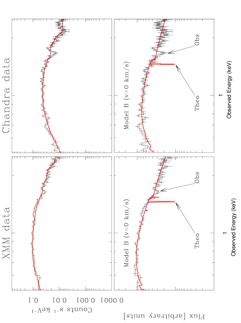
Figure 2: Instrument convolved (top), and physical model (bottom) of Model B applied to the XMM-Newton data (left) and Chandra data (right).

In fact, there is an important mismatch between theory and data. The statistical evidences can easily be read out from Table 2. The local $\chi^{2}_{(1-2\leavevmode\nobreak\ {\rm keV})}$ for XMM-Newton (Chandra) is 55.5 for 35 d.o.f (65.5 for 52 d.o.f), resulting in $P_{(1-2)\leavevmode\nobreak\ {\rm keV}}[{\rm Model\leavevmode\nobreak\ B};{\it XMM-Newton}]=0.01$ and $P_{(1-2)\leavevmode\nobreak\ {\rm keV}}[{\rm Model\leavevmode\nobreak\ B};{\it Chandra}]=0.1$. These probabilities locate Model B, very close to the rejection limit (a common threshold to reject the null hypotheses is $P_{\nu,\chi^{2}}\leq 0.05$).

Table 2: XSTAR fit results and comparison between sets of data. XMM-Newton vs Chandra observation of APM 08279+5255.

Parameter	XMM data	Chandra data
Model A: Fe fixed to solar; 0 km ${\rm s}^{-1}$
$\Gamma$	$2.11_{-0.03}^{+0.03}$	$1.84_{-0.03}^{+0.03}$
Norma	$1.34_{-0.02}^{+0.02}\times 10^{-4}$	$1.08_{-0.02}^{+0.03}\times 10^{-4}$
$N_{H}$ (${\rm cm}^{-2}$)	$1.14_{-0.06}^{+0.07}\times 10^{23}$	$1.32_{-0.10}^{+0.14}\times 10^{23}$
$\log(\xi)$	$1.50_{-0.05}^{+0.06}$	$1.50_{-0.07}^{+0.08}$
$\chi^{2}$/(d.o.f)	339.7/(289)	241.3/(183)
$P_{{\rm global}}[{\rm Model\leavevmode\nobreak\ A}]$	$2\times 10^{-2}$	$2\times 10^{-3}$
$\chi^{2}(1-2\leavevmode\nobreak\ {\rm keV})$/(d.o.f)	79/(35)	91/(52)
$P_{(1-2\leavevmode\nobreak\ {\rm keV})}[{\rm Model\leavevmode\nobreak\ A}]$	$4\times 10^{-6}$	$3\times 10^{-4}$
Model B: Fe free to vary; 0 km ${\rm s}^{-1}$
$\Gamma$	$2.06_{-0.03}^{+0.03}$	$1.82_{-0.03}^{+0.03}$
Norma	$1.32_{-0.02}^{+0.03}\times 10^{-4}$	$1.11_{-0.02}^{+0.02}\times 10^{-4}$
$N_{H}$ (${\rm cm}^{-2}$)	$5.08_{-0.13}^{+0.20}\times 10^{22}$	$5.97_{-0.25}^{+0.38}\times 10^{22}$
$\log(\xi)$	$1.50_{-0.18}^{+0.03}$	$1.50_{-0.13}^{+0.05}$
Fe	$5.04_{-0.23}^{+0.44}$	$4.83_{-0.27}^{+0.63}$
$\chi^{2}$/(d.o.f)	310.1/(288)	204.1/(182)
$P_{{\rm global}}[{\rm Model\leavevmode\nobreak\ B}]$	$0.19$	0.14
$\chi^{2}(1-2\leavevmode\nobreak\ {\rm keV})$/(d.o.f)	55.5/(35)	65.5/(52)
$P_{(1-2\leavevmode\nobreak\ {\rm keV})}[{\rm Model\leavevmode\nobreak\ B}]$	0.01	0.10
Model C: Fe fixed to solar; outflow at 0.21c
$\Gamma$	$2.12_{-0.03}^{+0.03}$	$1.83_{-0.03}^{+0.03}$
Norma	$1.35_{-0.02}^{+0.02}\times 10^{-4}$	$1.06_{-0.02}^{+0.02}\times 10^{-4}$
$N_{H}$ (${\rm cm}^{-2}$)	$7.08_{-0.27}^{+0.30}\times 10^{22}$	$6.72_{-0.36}^{+0.41}\times 10^{22}$
$\log(\xi)$	$1.82_{-0.04}^{+0.04}$	$1.72_{-0.09}^{+0.08}$
$\chi^{2}$/(d.o.f)	351.2/(289)	246.5/(183)
$P_{{\rm global}}[{\rm Model\leavevmode\nobreak\ C}]$	$7\times 10^{-3}$	$1\times 10^{-3}$
$\chi^{2}(1-2\leavevmode\nobreak\ {\rm keV})$/(d.o.f)	89/(35)	101.2/(52)
$P_{(1-2\leavevmode\nobreak\ {\rm keV})}[{\rm Model\leavevmode\nobreak\ C}]$	$5\times 10^{-8}$	$1\times 10^{-5}$
Model D: Fe free to vary; outflow at 0.21c
$\Gamma$	$2.08_{-0.03}^{+0.03}$	$1.85_{-0.03}^{+0.03}$
Norma	$1.32_{-0.02}^{+0.02}\times 10^{-4}$	$1.13_{-0.03}^{+0.02}\times 10^{-4}$
$N_{H}$ (${\rm cm}^{-2}$)	$3.85_{-0.08}^{+0.08}\times 10^{22}$	$3.71_{-0.08}^{+0.09}\times 10^{22}$
$\log(\xi)$	$1.78_{-0.06}^{+0.06}$	$2.12_{-0.04}^{+0.04}$
Fe	$4.84_{-0.28}^{+0.30}$	$8.36_{-0.49}^{+0.53}$
$\chi^{2}$/(d.o.f)	333.7/(288)	207/(182)
$P_{{\rm global}}[{\rm Model\leavevmode\nobreak\ D}]$	0.03	0.11
$\chi^{2}(1-2\leavevmode\nobreak\ {\rm keV})$/(d.o.f)	71.4/(35)	62.6/(52)
$P_{(1-2\leavevmode\nobreak\ {\rm keV})}[{\rm Model\leavevmode\nobreak\ D}]$	$9\times 10^{-5}$	0.17

The error parameters are 90% confidence limits. (a) Power-law normalization, photons keV^-1cm^-2s^-1 at 1 keV in the observed frame.

Based on the last result, we went further and explored the possibility that the gas absorbing X-rays in APM 08279+5255 is outflowing at intermediate-to-relativistic velocities. For that purpose we have shifted the spectra , produced with our XSTAR-based ionization models, by an array of velocities, from 0.08$c$ to 0.30$c$, with 0.01$c$ of resolution, and fit in several ways the X-ray spectrum of APM 08279+5255, using the XMM-Newton and Chandra data.

Table 2, quotes the best-fit parameters of the four most interesting fits, in the context of the single-absorber model. Models A and B are models with Fe solar and Fe free to vary at $v_{out}=0$ km ${\rm s}^{-1}$, respectively. Then, we have Model C and Model D, with Fe solar and Fe free (respectively) at $v_{out}=0.21c$, for both sets of data, XMM-Newton and Chandra. The single-absorber model cannot be ruled out (instantaneously), but it does not give a consistent fit to both sets of data (Model B for XMM-Newton and Model D for Chandra). Therefore, we explore the possibility of a multi-component photoionization model. In Figs. 3 and 4, we plot the residuals between each model presented here and the data. The dashed lines are residuals from a two-absorbers model, which we discuss in the next section. A detailed physical discussion of these scenarios and its implications are given in Sect. 6.

Figure 3: Residuals (in sign(data-model)$\chi^{2}$) of our photoionization models A,B,C and D to the XMM-Newton data, in the band $(1-2)$ keV observed frame. Dashed line is the residual of the two-absorbers model. See text.

Figure 4: Residuals (in sign(data-model)$\chi^{2}$) of our photoionization models A,B,C and D to the Chandra data, in the band $(1-2)$ keV observed frame. Dashed line is the residual of the two-absorbers model. See text.

4.2 Two-Absorbers photoionization model

Now that we have explored how the single-absorber model fits the data, we can go further, and see if the data supports a multicomponent photoionization model. The simplest such model is a two-photoionized-absorbers model, and we investigate if the addition of an extra component to the best-fit single-absorber model is statistically significant. This two-absorbers model consists of: one component at $v=0$ km ${\rm s}^{-1}$ (rest-velocity component), and one at $v=0.18c$ (high-velocity component) . We take the best single-absorber model (from Table 2), selected as the best combination between global and local $P_{\nu,\chi^{2}}$. Model B is the best for XMM-Newton data and Model D is the best for the Chandra set. The addition of an extra component (high-velocity component for XMM-Newton and rest-velocity component for Chandra) significantly improves the fit compared to the single-absorber model at the greater than 99.9% confidence level in both cases (according to the $F$-test), both globally and locally.

First, we fit a two-absorbers model to each set of data separately and then we do it simultaneously, to check for inconsistencies between fits. In Table 3, we have the results for these three schemes (Cols. 2,3,4). Figures 5 and 6 present plots of the best-fit two-absorbers model over the Chandra and XMM-Newton data, respectively. The fits between data sets give different best-fit parameters at $\gtrsim 1\sigma$, for six out of the seven fitted parameters ($\log\xi[2]$ is fully consistent).

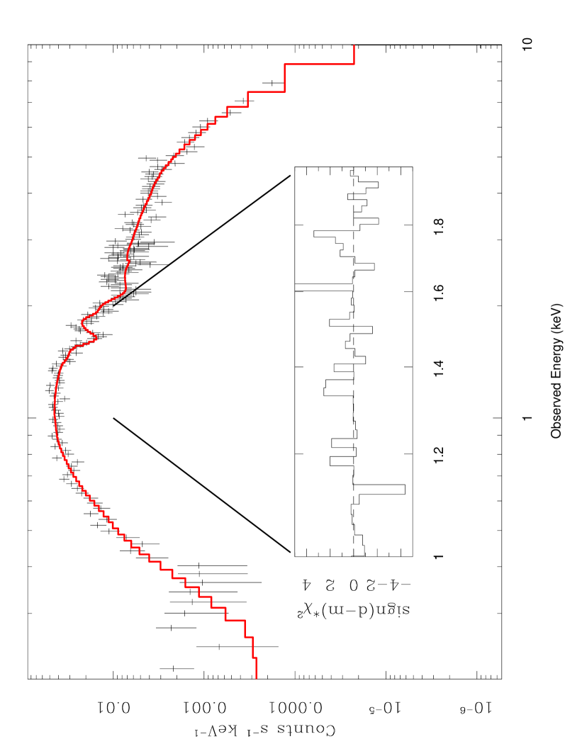
Figure 5: Chandra X-ray spectrum of APM 08279+5255 in the $0.2-10$ keV (observed frame) band.The solid thick line is the best-fit two-absorbers model. The inside plot shows the residual (in sign(data-model)$\chi^{2}$) for the $1-2$ keV band. This model gives good agreement on both sets of data.

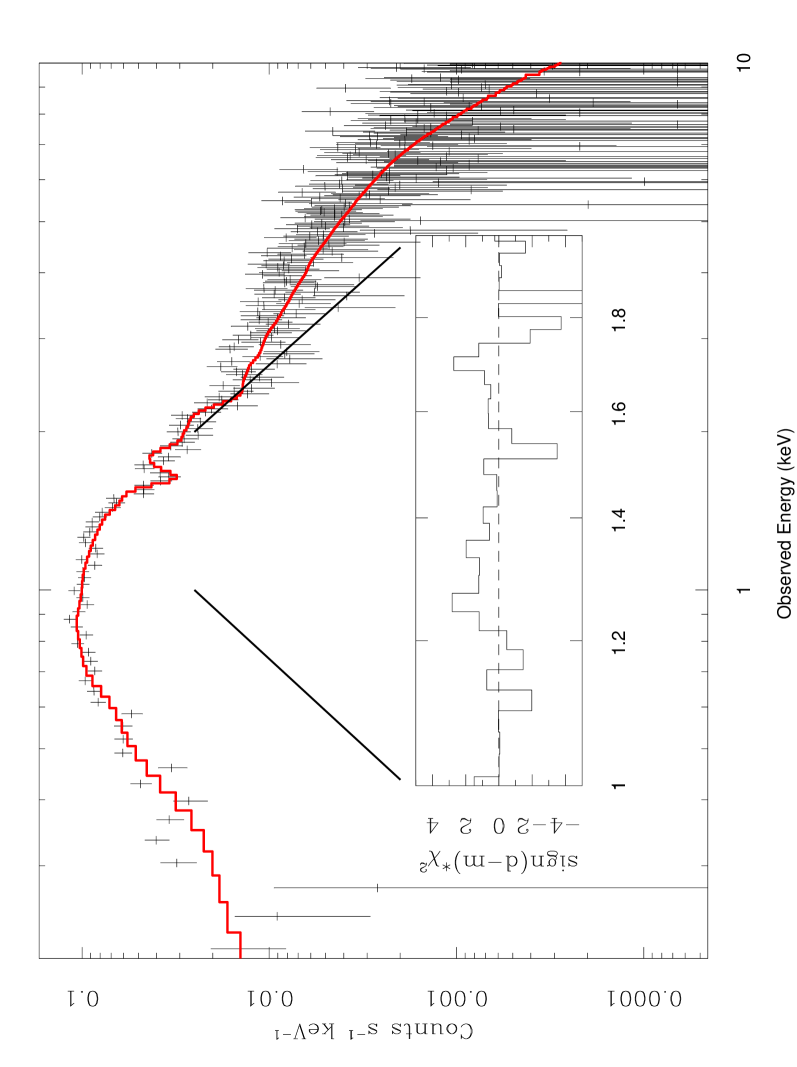
Figure 6: XMM-Newton X-ray spectrum of APM 08279+5255 in the $0.2-10$ keV (observed frame) band.The solid thick line is the best-fit two-absorbers model. The inside plot shows the residual (in sign(data-model)$\chi^{2}$) for the $1-2$ keV band. This model gives good agreement on both sets of data.

The two-absorbers model gives acceptable fits with high $\chi^{2}-$probability for both sets of data, but there exist small differences between best-fit parameters.

Table 3: Two-Absorber fits for XMM-Newton and Chandra.

Parameter	XMM	Chandra	Simult.	XMM	Chandra	XMM	Chandra
$\Gamma$	$2.08_{-0.03}^{+0.03}$	$1.84_{-0.02}^{+0.02}$	$2.00_{-0.01}^{+0.01}$	…	…	$2.13_{-0.02}^{+0.02}$	$1.83_{-0.02}^{+0.02}$
Norma	$1.41_{-0.03}^{+0.03}$	$1.18_{-0.02}^{+0.02}$	$1.34_{-0.01}^{+0.01}$	…	…	$1.50_{-0.02}^{+0.02}$	$1.17_{-0.02}^{+0.02}$
$N_{H}(1)$b	$5.72_{-0.19}^{+0.21}$	$6.05_{-0.19}^{+0.19}$	$7.34_{-0.15}^{+0.18}$	…	…	…	…
$\log\xi(1)$	$1.15_{-0.15}^{+0.14}$	$1.50_{-0.12}^{+0.03}$	$1.50_{-0.04}^{+0.02}$	…	…	…	…
Fe	$3.14_{-0.25}^{+0.27}$	$4.79_{-0.22}^{+0.23}$	$2.85_{-0.10}^{+0.10}$	…	…	…	…
$N_{H}(2)$b	$4.75_{-0.89}^{+1.20}$	$2.74_{-1.15}^{+0.68}$	$5.49_{-0.54}^{+0.71}$	…	…	…	…
$\log\xi(2)$	$3.03_{-0.04}^{+0.15}$	$3.10_{-0.12}^{+0.23}$	$3.00_{-0.01}^{+0.04}$	…	…	…	…
$\chi^{2}$/(d.o.f)	296.1/(286)	186.5/(180)	647.9/(473)	373.8/(293)	274.1/(187)	298.5/(291)	189.3/(185)
$P_{\rm global}[{\rm Two\leavevmode\nobreak\ Abs}]$	0.35	0.38	$4\times 10^{-8}$	$7\times 10^{-4}$	$2\times 10^{-5}$	0.39	0.43
$\chi^{2}(1-2\leavevmode\nobreak\ {\rm keV})$/(d.o.f)	44.9/(35)	48.9/(52)	135.1/(87)	65.7/(35)	69.4/(52)	43.9/(35)	49.3/(52)
$P_{(1-2\leavevmode\nobreak\ {\rm keV})}[{\rm Two\leavevmode\nobreak\ Abs}]$	0.14	0.65	$4\times 10^{-4}$	$7\times 10^{-4}$	0.05	0.17	0.63

The error parameters are 90% confidence limits. The Fe abundance is the same for both absorbers. (a) Power-law normalization, $\times 10^{-4}$ photons keV^-1cm^-2s^-1 at 1 keV in the observed frame. (b) Column density of the component, $\times 10^{22}$ ${\rm cm}^{-2}$.

If we fit both data sets simultaneously (Col. 4), we find reasonable consistency between them and the separated fits. The most notable discrepancy is seen in the power-law component, with differences of $\sim 10-15$% in its parameter values. To check for this difference, we have taken all the parameters resulting from the simultaneously fit and fixed them to each set of data separately (Cols. 5,6), and compute $\chi^{2}-$probabilities. In both cases, the fits are rejected (in both global and local senses). Finally, we have taken the simultaneous best-fit parameters and fixed them, except that we allowed the power-law parameters free to vary in each set of data (Cols. 7,8). We recover the goodness-of-fit and the model becomes acceptable. Then, we compute integrated observed fluxes (later in Sect. 6 we also compute intrinsic luminosities) using both set of data in the band $0.2-10$ keV with the following results: $F_{(0.2-10\leavevmode\nobreak\ {\rm keV})}[{\it Chandra}]=6.9\pm 0.3\times 10^{-13}$ ergs cm^-2 ${\rm s}^{-1}$and $F_{(0.2-10\leavevmode\nobreak\ {\rm keV})}[{\it XMM-Newton}]=7.6\pm 0.3\times 10^{-13}$ ergs cm^-2 ${\rm s}^{-1}$, thus the differences seen in the power-law component are reflected in a change of $\sim 10$ % on fluxes, and this could produce small changes in the physical parameters of the absorbers (the most notorious are $\log\xi(1)$, $\approx$ 30% and $N_{H}(2)$, $\approx$ 70%). However, the errors on the parameters allow us to obtain high $\chi^{2}-$probability if, appart from the power-law, both observations are fitted with the same physical two absorbers, opening the possibility that both absorbers have been there in both observations.

5 Line Identification

We are now in position of studying in more detail the possible identification of the feature $\sim 8$ keV (rest-frame) of the X-ray spectrum of APM 08279+5255. We will discuss two cases: i) the possible identification if we assume the single-absorber model is the best, and ii) the possible identification if we consider the two-absorbers model.

5.1 Case (i)

Given the good agreement between the Chandra data and our single-absorber model at $v\sim 0.21c$ (Model D of Table 2), we want to investigate how well constrained is the best-fit ionization parameter found and, its ability to reproduce the feature $\sim 8$ keV as well as the X-ray absorption at lower energies. For that purpose, we have taken one model in which the column density $N_{H}$ is fixed to $5\times 10^{22}$ ${\rm cm}^{-2}$, built a grid in $\xi$, $1.5\leq\log(\xi)\leq 4.5$ with resolution of 0.1, leaving the iron abundance free to vary, and computed $\chi^{2}$ produced by fitting our models at $v=0.21c$. The main result of this experiment is that clearly the Chandra data strongly favors $\log(\xi)\approx 2.1\pm 0.1$. For instance, at $\log(\xi)\approx 2.4$, there exists a clear deviation of the best-fit model from the data with $\Delta\chi^{2}\approx 70$, translated in that the model becomes rejected (from accepted). Thus, in Model D, the ionization state is mostly driven by the absorption at low energies, with an important contribution of the feature $\sim 8$ keV. Under these physical conditions, the feature is better represented by a complex of lines produced by L transitions of highly-ionized species of iron from Fe xviii to Fe xxii (Fe C2 in Table 4). The centroid of this complex is located $\sim$ 8.1 keV, i.e., $v\approx 0.21(\pm 0.01)c$.

Table 4: XSTAR spectral lines prediction.

Complex	Ion	Transition	$\lambda_{\rm lab}$	$\tau_{0}(\log[\xi]\approx 3)$	$\tau_{0}(\log[\xi]\approx 2.8)$	$\tau_{0}(\log[\xi]\approx 2.1)$
Fe C1 at	Fe xxv	1$s^{2}\leavevmode\nobreak\ {\rm{}^{1}S}-1s2p\leavevmode\nobreak\ {\rm{}^{1}P}$	1.85	110	44	$\ll 10^{-2}$
$N_{H}=5\times 10^{22}$ ${\rm cm}^{-2}$	Fe xxiv	1$s^{2}2s\leavevmode\nobreak\ {\rm{}^{2}S}-1s2s2p\leavevmode\nobreak\ {\rm{}^{2}P}$	1.86	33	36	$\ll 10^{-2}$
	Fe xxiii	2$s^{2}\leavevmode\nobreak\ {\rm{}^{1}S}-1s2p\leavevmode\nobreak\ {\rm{}^{1}P}$	1.87	45	108	$\ll 10^{-2}$
Fe C2 at	Fe xxii	2$s^{2}2p-1s2s^{2}2p^{2}\leavevmode\nobreak\ {\rm{}^{2}P}$	1.88		42	3
$N_{H}=5\times 10^{22}$ ${\rm cm}^{-2}$	Fe xxi	2$p^{2}-1s2s^{2}2p^{3}\leavevmode\nobreak\ {\rm{}^{3}S}$	1.89		10	5
	Fe xx	2$s^{2}2p^{3}-1s2s^{2}2p^{4}\leavevmode\nobreak\ {\rm{}^{4}P}$	1.91		3	18
	Fe xix	2$s^{2}2p^{4}-1s2s^{2}2p^{5}\leavevmode\nobreak\ {\rm{}^{3}P}$	1.92		0.4	26
	Fe xviii	2$s^{2}2p^{5}-1s2s^{2}2p^{6}\leavevmode\nobreak\ {\rm{}^{2}S}$	1.93		0.1	34

Two different complex of lines are predicted at different ionization states. The laboratory wavelength $\lambda_{\rm lab}$ is given in Å.

This identification is different from the one made by C02, who identify this feature as Fe xxv K lines. That identification is not based on a photoionization model, but on searching for the closest (and most conservative) line (with some other physical arguments), in likely several atomic data bases. The problem with the identification of this feature as Fe xxv lines (in our Model D), is that they required that the plasma be at $\log(\xi)\gtrsim 2.8$. Only at this highly-ionized state, the ionization fraction of ions like Fe⁺²², Fe⁺²³ and Fe⁺²⁴, are high enough to form spectral lines. In that physical scenario, a complex of lines (Fe C1), produced by transitions of iron ions from Fe xxiii to Fe xxv, arises naturally, where the K lines of Fe xxv are involved. However, our Model D at this $\log(\xi)\approx 2.8$ is a bad representation of the absorption at lower energies. In Fig. 7, we present the ionization fraction ($q_{i}$) of Fe ions from Fe xviii to Fe xxvi of our grid of XSTAR photoionized clouds at different $\log(\xi)$. At $\log(\xi)\approx 2.1$ ($\sim$ best-fit ionization parameter) the predominant ions are Fe ions from Fe xviii to Fe xxii, and the ionization fraction of Fe⁺²⁴ ($q_{\rm FeXXV}),is\sim 10^{-7}$. In Table 4 we present: the transitions contributing to the complex, the laboratory wavelength, and our XSTAR computation of the optical depth at the line core of each of these lines when the plasma is at these two ionization states (this gives a quantitative idea of the contribution to the complex).

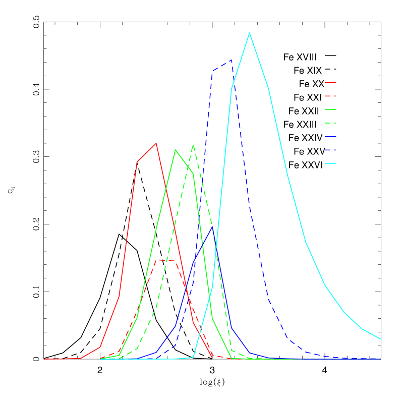
Figure 7: XSTAR ionization balance computation (ionization fraction $q_{i}$). Only shown in this plot species of Fe (xviii-xxvi). The single-absorber model favors $\log(\xi)\sim 2.1$, and the absorption feature at $\sim$8 keV rest-frame would be identified as the complex Fe C2 in Table 4. However, the HV component of the two-absorbers model strongly suggest that the feature can be associated to the Fe xxv K_α line ($\log(\xi)\sim 3$ is precisely where Fe⁺²⁴ has its peak).

5.2 Case (ii)

Nevertheless, after proving that the addition of a second component to the photoionized gas, is statistically required by the fits in both sets of data, we are able to support the identification of the feature as a Fe xxv line. The strongest evidence is that the high-velocity component is consistently fitted with an ionization parameter $\log\xi(2)\approx 3$. This is precisely where the peak of the ionization fraction of Fe⁺²⁴ is located. Therefore, we identify the absorption feature at $\approx 8$ keV as the complex Fe C1, in which the major contributor is the K_α line of Fe xxv. The physical implications are summarized in Sect. 6.

6 Discussion and Summary

We have found several interesting aspects in the X-ray spectrum of the QSO APM 08279+5255. The physical scenarios raised after the interpretation of Hasinger et al. (2002) as a Fe edge, and of Chartas et al. (2002) as relativistic ($\sim 0.2c-0.4c$) Fe xxv lines, have helped to scrutinize more closely the X-ray spectrum of this object. If we attempt to explain the spectrum by only investigating the full band $\sim 0.2-10$ k e V (observed frame), we find it hard to justify which model represents the data better in a statistical sense. After including a local criterion to evaluate the fits in the band $1-2$ k e V, we were able to converge to a model that accounts for both low- and high- energy spectral bands. Indeed, by modeling the spectrum with a photoionization model, which gives a better (over Gaussian lines alone for instance) representation of edges and absorption lines in the whole band $\sim 0.2-10$ keV, we are able to draw more physical information.

We discuss the implications of our results from Sect. 4 in two parts: (i) Assuming that the X-ray spectrum of APM 08279+5255 can be modeled by a single-absorber photoionization model. (ii) Assuming that the best representation of the spectrum is a two-absorbers model.

(i) Changes in the physical and kinematical state of the absorber: We see that the XMM-Newton data is represented by a highly-photoionized gas with column density $\sim 10^{23}$ ${\rm cm}^{-2}$, and $\log(\xi)\sim 1.5$ at 0 km ${\rm s}^{-1}$ in the frame of the quasar. Nevertheless, by allowing iron to be higher than solar (model B), we obtain a iron abundance best-fit value of ${\rm Fe}=5.04^{+0.44}_{-0.23}$, and the ionized gas column no longer needs to be as high as $10^{23}$ ${\rm cm}^{-2}$, but $\sim 5\times 10^{22}$ ${\rm cm}^{-2}$ instead, statistically improving the fit at 99% of significance over model A (with the same number of parameters than the absorbed power-law modified by an edge), similar to the H02 interpretation.

But $\sim$ 2 weeks before (in the frame of the quasar), the Chandra spectrum presented evidence of a material outflowing $\sim 0.21c$, not only showing an absorption-line-like feature at $\sim 8.1$ keV (rest-frame), but also pointing to absorption at lower energies $\sim 0.8-2$ keV (rest-frame), coming from species of iron from Fe xviii to Fe xxiv, and H- and He-like ions of Ne, Mg, Si, S, and O. In this context, the Chandra data appears to be pointing to (through model D): (a) a change in the kinematical state of the absorbing material, or more plausible, change in the projection of the velocity field on our line of sight (which would yield to the same effect), from $\sim 0.21c$ to $\sim$ 0 km ${\rm s}^{-1}$ (since the Chandra observation was made first than the XMM-Newton observation); and (b) a slight but noticeable change in the ionization state of the gas, from $\log(\xi)\sim 2$ to $\log(\xi)\sim 1.5$ in a timescale of $\sim 2$ weeks in the frame of the quasar. However, we find it physically hard to explain the deceleration shown by this model, in addition to a change in the ionization state of the gas without a significant change in the intrinsic luminosity of the source, and once we found the two-absorbers model statistically superior, we ruled out (i) and focused on (ii).

(ii) Both absorbers have been there: The two-absorbers model consists of: one absorber at $v=0$ km ${\rm s}^{-1}$, $N_{H}(1)=7.34_{-0.15}^{+0.18}\times 10^{22}$ ${\rm cm}^{-2}$, $\log\xi(1)=1.50_{-0.04}^{+0.02}$, and a second absorber at $v=0.18c$, $N_{H}(2)=5.49_{-0.54}^{+0.71}\times 10^{22}$ ${\rm cm}^{-2}$, $\log\xi(2)=3.00_{-0.01}^{+0.04}$ (parameters coming from the simultaneous best-fit). The chemical composition of both is the same, solar in all the elements (see model composition in Sect. 4) except in the abundance of iron ${\rm Fe}=2.85_{-0.10}^{+0.10}$. It is worth mentioning that from the separated fits, the two observations show a change in the power-law of $\approx 10$% and also show changes in the physical parameters. However, they (individually) change little (i.e, no large difference within errors); $\log\xi(1)$, from $\approx$ 1.2 to 1.5 ($\approx$ 30%); $N_{H}(1)\times 10^{22}$ ${\rm cm}^{-2}$, from $\approx$ 5.7 to 6.1 ($\approx$ 10%); $\log\xi(2)$, from $\approx$ 3 to 3.1 ($\approx$ 3%); $N_{H}(2)\times 10^{22}$ ${\rm cm}^{-2}$, from $\approx$ 4.8 to 2.7 ($\approx$ 70%, but see errors). The computation of $\chi^{2}$, on the other hand, is very sensitive to the continuum level, and small changes in the power-law are easily detected by the minimization-$\chi^{2}$ routine. We do not think this is a fundamental physical change of state between observations. At the moment these data do not allow us to discriminate whether the changes seen in the physical parameters are significant (within $\approx 2\sigma$) or not. Apparently, apart from the power-law component, both observations can be represented by the same two-absorbers model.

We have verified that the overabundance of Fe can be established respect to the abundance of oxygen (since it is the Fe/O ratio, which is cosmologically relevant), by comparing the observed spectra with the synthetic theoretical spectra at low-energies, if we increase the oxygen abundance. The ratio Fe/O must be $\approx 3$ in order to obtain acceptable fits in the low-energy band. This was first noticed by Hasinger et al. (2002), and its cosmological implications are discussed in Komossa & Hasinger (2003), based on chemical evolution studies of Hamann & Ferland (1993).

This multi-component photoionization approach has been successfully applied to other AGNs in different bands (X-ray and UV): NGC 3783 (Netzer et al. 2003; Krongold et al. 2003; Gabel et al. 2005); Mrk 279 (Fields et al. 2007; Costantini et al. 2007); NGC 4593 (Steenbrugge et al. 2003); NGC 985 (Krongold et al. 2005); MR 2251$-$178 (Kaspi et al. 2004); NGC 4051 (Kraemer et al. 2006; Armentrout et al. 2007; Krongold et al. 2007), a survey of a sample of 15 Type I AGNs can be found in McKernan et al. (2007). We will treat, this multi-component photoionization approach, as the best solution for our problem. However, note that a key difference with some of these cited papers is that the solution for APM 08279+5255 requires two unrelated absorbers at very different velocities.

A plausible framework in which to place these observational clues is in accretion disk wind models (Murray et al. 1995; Elvis 2000; Proga et al. 2000; Proga 2007). Recent high-resolution spectroscopy of APM 08279+5255, shows UV BALs in a wide range of velocities ($5\,000\lesssim v\lesssim 12\,000$ km ${\rm s}^{-1}$) and ionization degrees (ions like C vi, O vi, N v and Si iv), implying that the outflow may be composed of multiple components, with velocity; density and/or ionization parameter gradients (Srianand & Petitjean 2000). In particular, the model proposed by Elvis (2000) predicts that the UV BAL is formed in the conical section of a funnel-shaped flow ranging velocities $10\,000\lesssim v\lesssim 60\,000$ km ${\rm s}^{-1}$, (or up to $\sim 0.2c$ in our context). Furthermore, the model is very specific as to the location and physical properties of the X-ray absorbing material. The warm highly-ionized medium has column densities of $\sim 10^{22.5}$ ${\rm cm}^{-2}$, and temperatures of $\sim 10^{6}$ K, right pressure, and ionization parameter to ensure pressure equilibrium with the BELR clouds. Our XSTAR-based photoionization model estimates that the high-ionization, high-outflow velocity component (HV component), $\log(\xi)\approx 3$ has a temperature $T\sim$ few times $10^{6}$ K, and the best-fit column density $N_{H}(2)\sim 10^{22.5}$ ${\rm cm}^{-2}$, nicely consistent with the main physical properties of the warm highly-ionized medium. The low-ionization rest-frame velocity component (RV component) with $\log(\xi)\approx 1.5$ has a temperature $T\sim$ $10^{5}$ K, in accordance with the temperature of $\sim$ few times $10^{5}$ K found by Kaastra et al. (1995) in NGC 5548, and the degree of ionization is consistent with $\log(U)\sim 0.3$ reported by Mathur et al. (1995) for the same object, where a test to unify UV/X-ray absorbers in Seyfert galaxies was successfully applied.

Recalling the definition of the ionization parameter $\xi=L_{\rm ion}/(nR^{2})$, where $L_{\rm ion}$ is ionizing luminosity, $n$ is the gas density, and $R$ is the location of the absorber, we are able to compute the product of two un-observable quantities $(nR^{2})$ from the observable $\xi$ and $L_{\rm ion}$. We measured an intrinsic X-ray luminosity of $L_{\rm x}=1.12(\pm 0.04)\times 10^{47}k^{-1}$ ergs ${\rm s}^{-1}$, $k$ being the lensing magnification factor. With this we have: $(nR^{2})$[HV]$=1.12(\pm 0.11)\times 10^{44}k^{-1}$ cm^-1 and $(nR^{2})$[RV]$=3.54(\pm 0.11)\times 10^{45}k^{-1}$ cm^-1. This is the first time this quantity is measured for this BAL QSO (since it is the first time $\xi$ is properly constrained). Despite we still are not able to break the natural degeneracy between $n$ and $R$ (due to lack of variability), it allows us to present order-of-magnitude estimates on the mass-loss rate and energy budgets of the system. Assuming the HV forms part of the high-ionization BAL flows, which reaches velocities up to $\sim 0.2c$ (see Rodriguez Hidalgo et al. 2007, for a recent review of high velocity (HV) outflow in quasars), and that the X-ray absorber in APM 08279+5255 is part of the conical section of the funnel-shaped flow proposed by Elvis (2000) (although this estimation is independent of this specific geometry and can be equally applied to a spherical shell of gas for instance, without significatively changing the final conclusions), which forms a shell with covering factor $f_{\rm cov}$ moving at a velocity $v$, we estimate the mass-loss rate for the system:

$$\dot{M}_{w}=4\pi\mu_{H}(nR^{2})vf_{\rm cov},$$ (4)

where $\mu_{H}$ is the mean mass per H atom. Using $(nR^{2})$[HV]$=1.12\times 10^{44}k^{-1}$ cm^-1, an outflow velocity $v=0.18c$ and assuming a covering factor of 0.01, we have a mass-loss rate of $\dot{M}_{w}\approx 2873k^{-1}$ $M_{\odot}\leavevmode\nobreak\ {\rm yr}^{-1}$. The total kinetic power released by the wind in APM 08279+5255 is $\dot{M}_{w}v^{2}/2=2.6\times 10^{48}k^{-1}$ ergs ${\rm s}^{-1}$. The accretion rate is related with the accretion luminosity with:

$$\dot{M}_{\rm acc}\approx 17\frac{L_{\rm bol}}{10^{47}\leavevmode\nobreak\ {\rm ergs\leavevmode\nobreak\ s^{-1}}}\frac{0.1}{\eta}M_{\odot}\leavevmode\nobreak\ {\rm yr}^{-1},$$ (5)

where $L_{\rm bol}$ is the bolometric luminosity, $\eta$ is the accretion efficiency (assumed to be $\sim 0.1$), and $c$ is the speed of light. With our measured $L_{\rm x}$ we are able to estimate $L_{\rm bol}=\beta L_{\rm x}$. We adopt a bolometric correction factor $\beta=20$, based on the mean AGN SED of Elvis et al. (1994). Explicitly, in terms of the lensing magnification factor, $\dot{M}_{\rm acc}\approx 340k^{-1}$  $M_{\odot}\leavevmode\nobreak\ {\rm yr}^{-1}$. This would lead to the conclusion that the central black hole in APM 08279+5255 accretes $\sim 1$ order of magnitude less matter than the estimated mass-loss rate. Recently, from high-resolution Chandra and XMM-Newton spectroscopic studies at least three systems show the property of having mass outflow rates $\sim 1$ order of magnitude larger than the accretion rates (at $\sim$ 10% efficiency): the micro-quasar GRS 1915+105 (Lee et al. 2002b), the Seyfert 1 galaxy MCG-6-30-15 (Turner et al. 2004; Sako et al. 2003; Lee et al. 2002a), and the Seyfert 2 galaxy IRAS 18325-5926 (Lee 2005). However, we are aware of two major sources of uncertainties in these estimations. Due to its location, the uncertainty in $f_{\rm cov}$ is large because the exact geometry in the base of the outflow is not known. On the other hand, the bolometric correction factor could be larger than the one used here, locating $\dot{M}_{\rm acc}$ and $\dot{M}_{w}$ in the same order of magnitude. Either we detect the outflow in a very small period of activity (which would be very fortuitous) or the outflow plays a major role in the process of sending matter back to the interstellar medium (e.g., Crenshaw et al. 2003; Lee 2005; Krongold et al. 2007). If we assume that the mass of the black hole $M_{\rm BH}\approx 2\times 10^{10}$ $M_{\odot}$, (as estimated by Shields et al. 2006), the ratio $L_{\rm bol}/L_{\rm edd}\approx 0.8k^{-1}$ (where $L_{\rm edd}$ is the Eddington luminosity). This number is in accordance with the general trend of low $L_{\rm bol}/L_{\rm edd}$ ratio for BALQSOs reported by Boroson (2002). With these estimations, we can derive the launching radius $r_{\rm launch}$ for a radiatively-driven wind:

$$r_{\rm launch}\approx\frac{2GM_{\rm BH}}{v^{2}}\left(\Gamma_{f}\frac{L_{\rm UV}}{L_{\rm edd}}-1\right).$$ (6)

Here, we have used the relation $v\leavevmode\nobreak\ vs\leavevmode\nobreak\ r$ for a radiatively-driven steady wind and assumed that at very large radii the flow has reached a terminal velocity $v$. Assuming that the wind is driven by a UV luminosity $L_{\rm UV}\sim 4\times 10^{46}$ ergs ${\rm s}^{-1}$, with a force multiplier $\Gamma_{f}\sim 100$ (taken from Laor & Brandt 2002), and using a flowing velocity $v=0.18c$, we find $r_{\rm launch}\approx 7\times 10^{16}$ cm. On the other hand, if we use the maximum observed velocity of the UV absorber (through the C vi line), for this quasar of $v=0.041c$, we find $r_{\rm launch}\approx 1\times 10^{18}$ cm. One possible explanation for the difference in the two distances, is that the UV absorber is at a lower ionization state, lying in the low ionization BAL region of the funnel-shaped flowing (for visual help see Fig. 5 of Elvis 2000), and more specifically in the large radii part in which the UV absorber has reached its highest (terminal) velocity. A rigorous study of the hydrodynamical properties of the X-rays/UV absorbers in AGN is beyond the scope of this paper. However, the simplistic approach used in this analysis could be useful as a framework for future works on the study of the central region of this quasar.

To summarize, the absorbing gas in APM 08279+5255 can be represented by a two-absorbers model with column densities $N_{H}(1)\approx 7\times 10^{22}$ ${\rm cm}^{-2}$, $N_{H}(2)\approx 6\times 10^{22}$ ${\rm cm}^{-2}$, ionization parameters $\log\xi(1)\approx 1.5$ and $\log\xi(2)\approx 3$, with one of them (the HV component) outflowing at $v\approx 0.18(\pm 0.01)c$, carrying large amount of gas out of the system. The feature at $\sim 8$ keV (rest-frame) is fully predicted and reproduced by our photoionization model, to be a complex of Fe lines coming from high state of ionization, in which the main contributor is the Fe xxv $\lambda 1.85$ Å, improving the characterization of the kinematics and the quantitative evolution analysis of this high $z$ quasar. We confirm evidence for an overabundance of Fe/O, from the XMM-Newton observation of this quasar (previously inferred and discussed in Hasinger et al. 2002; Komossa & Hasinger 2003, based on calcutations of Hamann & Ferland 1993). The analysis is made for the first time on the Chandra observation of APM 08279+5255, implying that both absorbers require Fe/O supersolar, placing similar constraints on models as before, and additionally shows that both independent absorbers have a similar chemical history.